Phase Retrieval via Sensor Network Localization
The problem of phase retrieval is revisited and studied from a fresh perspective. In particular, we establish a connection between the phase retrieval problem and the sensor network localization problem, which allows us to utilize the vast theoretica…
Authors: Sherry Xue-Ying Ni, Man-Chung Yue, Kam-Fung Cheung
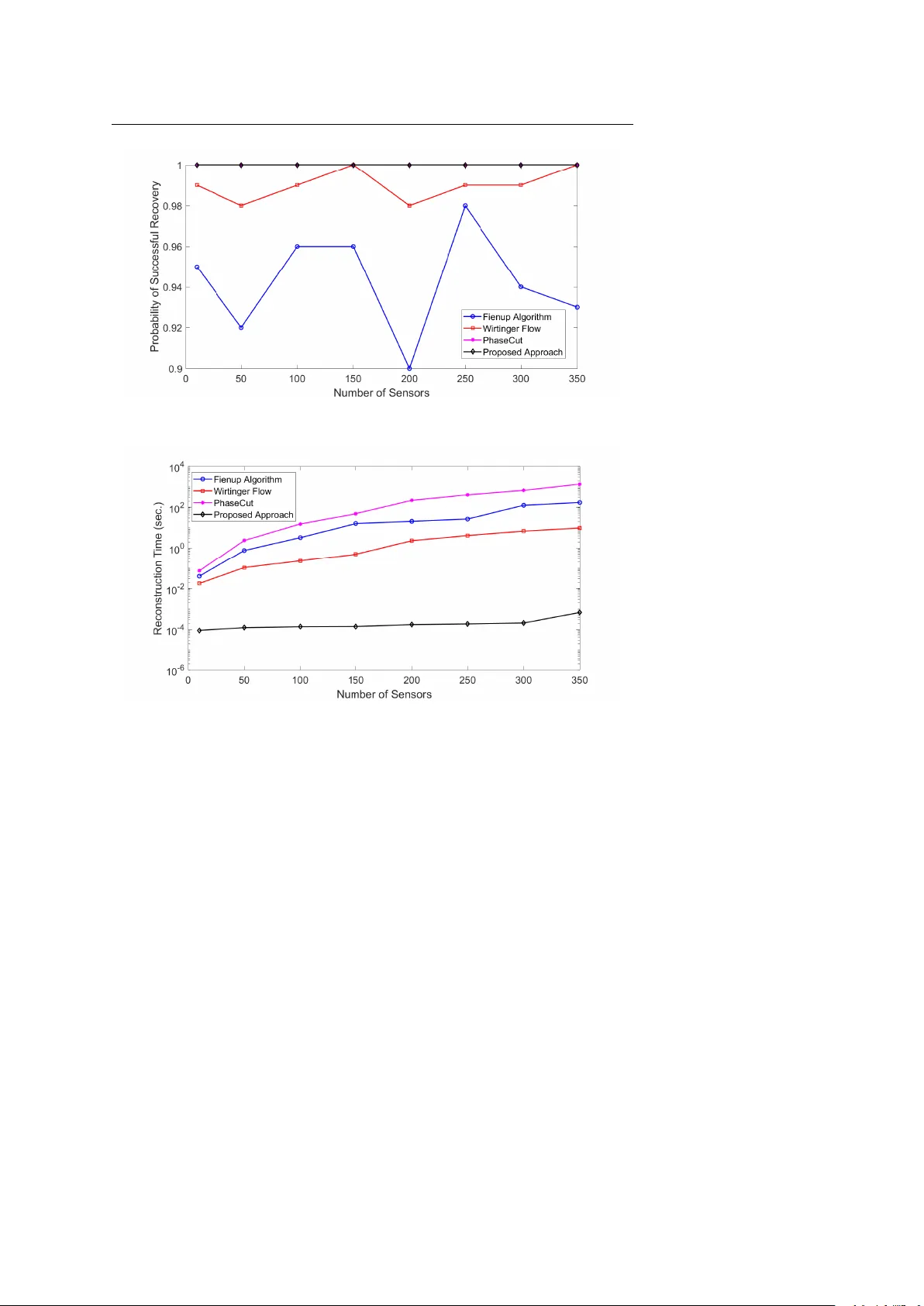
Noname man uscript No. (will b e inserted b y the editor) Phase Retriev al via Sensor Net w ork Localization Sherry Xue-Ying Ni · Man-Ch ung Y ue · Kam-F ung Cheung · An thon y Man-Cho So Received: date / Accepted: date Abstract The problem of phase retriev al is revisited and studied from a fresh p ersp ectiv e. In particular, w e establish a connection betw een the phase re- triev al problem and the sensor netw ork lo calization problem, which allows us to utilize the v ast theoretical and algorithmic literature on the latter to tackle the former. Lev eraging this connection, we develop a tw o-stage algorithm for phase retriev al t hat can pro v ably reco v er the desired signal. In b oth sparse and dense settings, our prop osed algorithm impro ves upon prior approaches sim ultaneously in the num ber of required measuremen ts for recov ery and the reconstruction time. W e presen t numerical results to corrob orate our theory and to demonstrate the efficiency of the proposed algorithm. As a side re- sult, we prop ose a new form of phase retriev al problem and connect it to the complex rigidit y theory prop osed by Gortler and Thurston [14]. Sherry Xue-Ying Ni Department of Systems Engineering and Engineering Managemen t, The Chinese University of Hong Kong T el.: +852 3943-8313 F ax: +852 2603-5505 E-mail: xyni@se.cuhk.edu.hk Man-Chung Y ue Imperial College Business School, Imperial College London, United Kingdom E-mail: m.yue@imp erial.ac.uk Kam-F ung Cheung Department of Systems Engineering and Engineering Management, The Chinese University of Hong Kong E-mail: kfcheung@link.cuhk.edu.hk Anthon y Man-Cho So Department of Systems Engineering and Engineering Management, The Chinese University of Hong Kong E-mail: manchoso@se.cuhk.edu.hk 2 Sherry Xue-Ying Ni et al. 1 Introduction 1.1 Phase Retriev al Problem The problem of phase retriev al consists of recov ering a signal v ector x ∈ C n from phaseless in tensity measurements of the form |h x, φ m i| 2 = b m , m = 1 , 2 , . . . , M , (1) where for each m = 1 , . . . , M , b m ∈ R + is the observed output of the intensit y measuremen t asso ciated with a giv en measurement v ector φ m ∈ C n . A collec- tion Φ = { φ m } M m =1 of measurement vectors is called an ensem ble. Throughout the pap er, we fo cus on the setting where w e can freely design these measure- men t v ectors Φ . As w e will see, the design of the ensemble Φ is of utmost imp ortance to the reco v ery pro cedure. Note that for an y unit-modulus com- plex num b er e iθ , the vector e iθ x yields the same measuremen ts. Therefore, we could reco ver the signal x only up to the equiv alence relation ∼ given by x ∼ y if and only if y = e iθ x for some θ ∈ R . Let C n / ∼ b e the set of equiv alence classes induced b y the equiv alence relation ∼ and denote by A Φ : C n / ∼→ R + the intensit y map associated with the ensem ble Φ = { φ m } M m =1 ; i.e., ( A Φ ( x )) m = |h x, φ m i| 2 , m = 1 , . . . , M . (2) F or simplicity , w e will write A in place of A Φ when the ensem ble Φ is clear from the con text. The phase retriev al problem has a long history and receiv ed great atten tion due to its v ast mo delling p ow er in man y areas. Fields of applications include X-ra y and crystallography imaging [15], quantum optics [20], astronomy [10], acoustics [2], and microscopy [19]. F or more discussions on the history , appli- cations, and recen t dev elopments of phase retriev al, w e refer the readers to the excellen t surveys [18, 26]. 1.2 Related W ork Ov er the past few decades, the phase retriev al problem has b een extensiv ely studied in the literature. A p opular approac h in practice is to use the so- called error reduction-type algorithms. Algorithms that fall in to this class, including the famous Gerch berg-Saxton algorithm [13] and the Fien up algo- rithm [10 – 12], are essen tially alternating pro jection-type algorithms [18]. The adv an tage of this approach is its relativ ely low computational complexit y and flexibilit y in incorp orating prior knowledge of the signal into the recov ery pro cess. Unfortunately , this approach often lacks pro v able con vergence guar- an tees and suffers from the issues of multiple stationary p oin ts and instability , Phase Retriev al via Sensor Netw ork Localization 3 esp ecially with non-conv ex priors [18]. Another weakness is that the n um- b er of measuremen ts required when using these algorithms is not known a priori, though some efforts to remedy this hav e been made in [21]. In par- ticular, Netrapalli et al. [21] studied a version of the alternating pro jection metho d for the phase retriev al problem. Their algorithm recov ers the signal using O ( n log 3 n log(1 / )) intensit y measuremen ts and has computational com- plexit y O ( n 2 log n (log 2 n + log 2 1 log log 1 )). How ev er, this is still far from ex- plaining the empirical success of error reduction-t yp e algorithms and a rigorous mathematical foundation for this approac h remains elusive. Another recen t approach is based on semidefinite programming and con v ex relaxation. The basic idea of this approach is to interpret quadratic measure- men ts (1) as linear measurements of a rank-one matrix X = xx H . Then, the phase retriev al problem can b e equiv alen tly rewritten as a rank-minimization problem. Subsequently , by using a conv ex surrogate suc h as the trace norm to replace the rank function, w e obtain a semidefinite program that can be solv ed in polynomial-time by off-the-shelf solvers. PhaseLift prop osed b y Cand ` es et al. [7] and PhaseCut b y W aldspurger et al. [29] are examples of suc h an ap- proac h. The dra wbac k of this approach is its high computational complexity . Indeed, the complexities of PhaseLift and PhaseCut to return a solution of accuracy are O ( n 3 / 2 ) and O ( n 3 / √ ), resp ectively . Both metho ds use an en- sem ble of O ( n log n ) i.i.d. standard n -dimensional Gaussian random vectors. Assuming the signal x is s -sparse (i.e., x has at most s non-zero comp onents), the ` 1 -regularized version of PhaseLift [17] impro v es the num ber of required Gaussian measuremen ts to O ( s 2 log n ). Nonetheless, this algorithm again re- quires solving a semidefinite program and hence has a similar computational complexit y as PhaseLift and PhaseCut. Therefore, this approach is not appli- cable to large-scale phase retriev al problems in practice. Other approaches usually inv olv e construction of sp ecial matrices. In [16], Iw en et al. constructed blo ck circulant measurement matrices that can b e blo c k diagonalized. By constructing certain inv ertible blo ck circulant matri- ces, one can express the av ailable squared magnitudes as a system of linear measuremen ts, thereby recov ering the signal. The approach reduces compu- tational complexity to O ( n (log 3 n log 3 (log n ))); whereas the ensemble size is still as large as O ( n log 2 n log 3 (log n )) to guarantee unique recov ery with high probabilit y . In a recen t w ork [6], a non-con vex approach based on Wirtinger flo w w as introduced to extract phase information from few er random mea- suremen ts. The num ber of measurements and complexit y of this algorithm are b oth O ( n log n ). In [23], the authors studied the general compressive phase re- triev al problem with sparsit y s . They developed a no v el approac h based on a sparse-graph co ding framework and can recov er a random fraction of non-zero comp onen ts with 14 s measurements and complexit y Θ ( s ). Nevertheless, their metho d is only capable of correctly recov ering part of the non-zeros en tries and they still require 4 s − o ( s ) measurements. There ha ve also b een endea vours to understand the minim um size of an ensem ble so that the measurements uniquely determine the signal up to the equiv alence relation; i.e., the in tensit y map A is injectiv e. T o wards that end, 4 Sherry Xue-Ying Ni et al. Bandeira et al. [4] conjectured that 4 n − 4 generic measurement v ectors are b oth necessary and sufficient for the injectivity of the intensit y map and sho wed in the same paper that the conjecture is true when n = 2 and n = 3. This conjecture is now known as the 4 n − 4 conjecture. The sufficiency was pro ved b y Fic kus et al. in [9]. One suc h ensem ble consisting of 4 n − 4 determin- istic measurements w as constructed in [24] via a low rate sampling metho d. Unfortunately , the necessary part of the conjecture is false—an ensem ble ˆ Φ of 11 4-dimensional measurement v ectors whose intensit y map A ˆ Φ is injective w as constructed in [28]. 1.3 Our Approac h and Main Contributions Our work sets out with the in teresting observ ation that the phase retriev al problem can b e seen as a sensor netw ork lo calization problem. More precisely , eac h component of the signal x can be view ed as a point (whic h we will refer to as sensors ) in d -dimensional Euclidean space, where d = 1 for real signals and d = 2 for complex signals. If w e explicitly design intensit y measuremen ts to form edges joining these sensors, then determining x can b e viewed as lo calizing the sensors in space. F urthermore, if the underlying graph generated by these measuremen ts satisfies certain rigidit y property , then eac h en try of x can b e uniquely determined up to the equiv alence relation. In this work, we will design a deterministic measurement ensem ble that fulfils the rigidity requiremen t and aim to construct an injectiv e mapping with as few measurements as p ossible. Our contribution is threefold. First, w e establish a connection b et ween the phase retriev al problem and the w ell-studied sensor netw ork localization prob- lem. This allo ws us to use the to ols from rigidit y theory and graph realization to b ear on the phase retriev al problem. In particular, w e prop ose a t w o-stage algorithm to uniquely recov er all phases up to the equiv alence relation ∼ with few measuremen ts. Concretely , w e design a deterministic ensem ble such that the underlying graph generated by intensit y measurements is a d -lateration graph that is univerally rigid. By rigidit y theory and relev ant results in [31], w e can easily obtain prov able guaran tee for unique recov ery . F or the non-sparse phase retriev al problem, our prop osed ensem ble consists of only 3 n − 2 mea- suremen ts and the corresponding in tensity map is injective. F or the sparse case where there are at most s non-zero comp onen ts, the n umber of measurements is further reduced to n + 2 s − 2. Injectivity of our mapping is demonstrated b y theoretical analysis. The algorithm is easy to implement and allows paral- lel computation. Simulations further demonstrate its efficacy and superiority o ver b enchmark approaches in terms of efficiency . The computational com- plexit y scales only linearly with n . T o the b est of our knowledge, this is the first work to study the phase retriev al problem b y incorp orating results from rigidit y theory . Second, our ensemble design yields an injective intensit y map of minimal size, and we provide explicit constants for the num ber of measure- men ts. Last but not least, w e propose a new v ariant of the phase retriev al Phase Retriev al via Sensor Netw ork Localization 5 problem and connect it to the complex rigidity theory proposed by Gortler and Th urston [14]. It should b e p ointed out that our approach does not constitute a counter- example to the necessary part of the 4 n − 4 conjecture. In particular, the conjecture claims that the ensem ble of any injectiv e intensit y map is of size at least 4 n − 4. The injectivit y is understo o d as a map on the whole C n / ∼ , whereas our prop osed algorithm prov ably reco v ers the correct signal with an additional minor assumption on the true signal. Neverth eless, as we will see in Section 3, our metho d fails only for those signals that hav e its first t w o comp onen ts collinear with the origin. W e also remark that a differen t ensem ble of the same size app eared in an unpublished man uscript [22]. Ho w ev er, they did not provide motiv ations and insigh ts for their ensem ble, and the injectivity of the corresp onding in tensity map is not clear. 1.4 Organization The remainder of the pap er is organized as follows. Section 2 is devoted to revisiting the theory of sensor net work lo calization and graph rigidit y , whic h constitutes the fundamental basis for our approac h. Section 3 focuses on our no vel approac h to the phase retriev al problem, including a rigidity-theoretic t wo-stage algorithmic framework applied to the phase retriev al problem and a theoretical analysis to demonstrate the injectivity of the measurement ensem- ble generated by our algorithm. W e then provide n umerical results in Section 4 to v alidate our theoretical findings, where w e compare against three meth- o ds in the literature; namely , the Fienup algorithm [12], the Wirtinger flow algorithm [6], and PhaseCut [29]. In Section 5, we study the complex rigid- it y theory and its connection to complex-measuremen t-based phase retriev al problems. Finally , we conclude the pap er in Section 6. Throughout the pap er, the vectors are column v ectors unless sp ecified oth- erwise; e j denotes the j -th standard co ordinate basis vector of suitable dimen- sion; ( · ) T and ( · ) H denote the transp ose and Hermitian transpose, respectively; h· , ·i refers to the inner product of v ectors; < ( · ) and = ( · ) denote the real and imaginary parts of a complex n umber or vector, resp ectively . 2 Sensor Netw ork Localization In this section, we review the sensor net w ork localization problem and a graph rigidit y-theoretic approach to tac kling it. Then, we present a nov el connection b et ween the phase retriev al problem and the sensor netw ork localization prob- lem. Suc h a connection allows us to utilize p o w erful results in rigidit y theory to design the measurement ensem ble that yields a minimal-size injectiv e in tensit y map. 6 Sherry Xue-Ying Ni et al. 2.1 Rigidit y Theory and Sensor Netw ork Lo calization The problem of sensor net work lo calization is among the classic topics in sig- nal pro cessing and arises when one is interested in determining the p ositions of no des in a netw ork from a set of measurements. W e do not attempt to giv e a comprehensive review, but only highlight the crucial findings of the relationship b et ween unique lo calizabilit y and graph rigidity theory . T o b egin, let us give a formal definition of the sensor netw ork lo calization problem. Consider a netw ork that consists of a n um b er of anchor no des whose p ositions are known, together with a num b er of sensor nodes whose lo cations are to b e estimated. Let d b e the dimension of the Euclidean space in which these no des reside. Let G = ( V , E ) b e the given netw ork, where V and E denote the vertex set and the edge set of the graph, resp ectively . Without loss of generality , we assume that G is connected. The vertices can b e partitioned in to tw o categories: the set V s = { 1 , . . . , n } of sensors, and the set V a = { n + 1 , . . . , n + m } of anchors. In particular, the p ositions of anchors are given b y the v ector u ∈ R dm . F or the sak e of clarity , w e define three subsets of E , namely E aa , E sa , and E ss , which are defined as E aa = { ( i, j ) ∈ E : i, j ∈ V a } , E sa = { ( i, j ) ∈ E : i ∈ V s , j ∈ V a } , and E ss = { ( i, j ) ∈ E : i, j ∈ V s } , resp ectiv ely . F or ( i, j ) ∈ E aa , the distances are trivially known; for ( i, j ) ∈ E sa or ( i, j ) ∈ E ss , the distances are acquired b y applying measuremen ts. The distances b etw een the no des are represented by positive weigh ts assigned to the edges, namely r ij for ( i, j ) ∈ E sa and ˜ r ij for ( i, j ) ∈ E ss . F or simplicity , we assume that all the measured data are noiseless. Let r ∈ R | E sa | and ˜ r ∈ R | E ss | b e the collection of distance measurements. Then, an instance of the sensor net work lo calization problem is given b y ( G, ( r, ˜ r ) , u, d ). The ob jective is to find a p osition assignment x ∈ R nd to the sensor no des such that the following system is satisfied: k x i − x j k 2 = r ij , for ( i, j ) ∈ E sa ; k x i − x j k 2 = ˜ r ij , for ( i, j ) ∈ E ss ; x i ∈ R d , for i = 1 , . . . , n. Herein, the pair ( x, u ), whic h represents the p ositions of all no des in space, is called a lo c alization of G . One interesting question in this setup is whether and when the sensor p ositions x can b e uniquely determined. If an instance admits a unique lo calization in R d , we sa y that it is uniquely lo c alizable . Eren et al. [8] utilized to ols from rigidity theory to discuss the connection b etw een unique lo calizability and properties of the asso ciated net w ork. In particular, they stated that follo wing theorem. Theorem 1 (Unique Lo calizabilit y & Global Rigidity [8]) F or any d ≥ 1 , a generic sensor network lo c alization instanc e is uniquely lo c alizable if and only if its asso ciate d network G = ( V , E ) is glob al ly rigid. In graph theory , a graph G = ( V , E ) with p being its lo calization in R n is called glob al ly rigid if p is the unique (up to congruence) lo calization of G in Phase Retriev al via Sensor Netw ork Localization 7 n -dimensional Euclidean space. Nevertheless, it has been sho wn that even if an instance satisfies the global rigidit y property , the problem of estimating the p ostions is still in tractable in general [25]. T o ov ercome the barrier, So and Y e in tro duced the notion of unique d -lo calizability in [27], while Zh u et al. applied the notion of univ ersal rigidit y to strengthen the connection [31]. In particular, a generic sensor netw ork lo calization instance is called uniquely d -lo c alizable if it admits a unique lo calization in any Euclidean space with dimension ` ≥ d . A graph G = ( V , E ) with p b eing its lo calization in R n is called universal ly rigid if p is the unique (up to congruence) lo calization of G in any Euclidean space. The connection b etw een unique d -lo calizability and universal rigidit y is presen ted b elow. F or a rigorous pro of, readers can refer to [31, Theorem 2]. Theorem 2 (Unique d -Lo calizabilit y & Univ ersal Rigidity [31] ) F or any d ≥ 1 , a generic sensor network lo c alization instanc e is uniquely d -lo c alizable if and only if its asso ciate d network G = ( V , E ) is universal ly rigid. Although univ ersal rigidit y is more restrictive than global rigidity , it still cap- tures a host of net w orks. Examples of univ ersally rigid graphs include complete graphs and d -lateration graphs. The latter notion is defined as follows. Definition 1 ( d -lateration Graph [1]) L et d, n ≥ 1 b e inte gers with n ≥ d + 1 . Then, an n -vertex gr aph G = ( V , E ) is c al le d a d -later ation gr aph if ther e exists an or dering { 1 , 2 , . . . , n } of the vertic es in V such that (i) the first d + 1 vertic es 1 , 2 , . . . , d form a c omplete gr aph; (ii) every vertex j ≥ d + 1 is c onne cte d to at le ast d + 1 of the vertic es 1 , 2 , . . . , j − 1 . In particular, a sensor netw ork localization instance is uniquely d -lo calizable if its associated netw ork is a d -lateration graph. The pro of is given in [31, Theorem 3]. Next, we will apply this prop osition to design the measurement ensem ble for phase retriev al. 2.2 Sensor Net work Lo calization and Phase Retriev al In this section, we consider the phase retriev al problem from a fresh p ersp ec- tiv e. In particular, we lo ok at the problem through the lens of the sensor net work lo calization problem. Concretely , each comp onent of the signal x can b e regarded as a sensor in d -dimensional Euclidean space, where d = 1 for real signals and d = 2 for complex signals; while the origin can b e viewed as an anc hor. Since w e assume that the measurement v ectors can be designed freely , w e restrict our attention to measurement v ectors of the forms φ k = e k (where 1 ≤ k ≤ n ) and ˜ φ j k = e j − e k (where 1 ≤ j < k ≤ n ) . (3) The former yields the distance b etw een sensor k and the origin (i.e., | x k | ), while the latter yields the distance betw een sensors j and k (i.e., | x j − x k | ). Th us, by choosing differen t subsets of measurement vectors from (3), we obtain differen t instances of the sensor netw ork lo calization problem. No w, consider an instance of the sensor netw ork lo calization problem constructed according 8 Sherry Xue-Ying Ni et al. to the abov e recipe, and let G b e the underlying graph. Based on results in the previous section, if G is univ ersally rigid, then the instance admits a unique lo calization in any Euclidean space. More precisely , all sensors are uniquely determined up to congruence in space, which implies unique recov ery of the reconstructed signal x . W e are thus motiv ated to construct an ensemble with as few measurement v ectors from (3) as p ossible, and y et the graph G induced b y these measurements is universally rigid. W e will discuss how this can b e ac hieved in the next section. 3 A Rigidity-Theoretic Approac h to Phase Retriev al Let x = ( x 1 , . . . , x n ) b e the signal v ector that w e wish to recov er. T o implemen t the idea in Section 2.2, we construct a graph G = ( V , E ), where the vertex set V is given b y V = { 0 , x 1 , . . . , x n } (here, we use x i to denote b oth the lab el of the vertex and its location in space) and the edge set E is obtained using the following pro cedure, so that G is a d -lateration graph ( d = 1 if x is a real signal and d = 2 if x is a complex signal). 1. Cho ose d + 1 no des from V as anchors and form a complete graph. 2. Consider the remaining no des as sensors. F or each sensor node, construct d + 1 edges connecting the sensor to all the anc hors. Since G is univ ersally rigid by construction, once the measurements corre- sp onding to the edges of G are a v ailable, the lo cations of the vertices are uniquely determined and so is the target signal vector. W e now propose a rigidit y-theoretic tw o-stage algorithm to actually reco v er the target signal v ector. W e will first illustrate the idea for real signals and then extend it to complex ones. 3.1 Real Phase Retriev al Consider the case where the signal x = ( x 1 , . . . , x n ) w e wish to reco v er is real; i.e., x i ∈ R for i = 1 , . . . , n . In this case, w e hav e d = 1. By Definition 1, t wo anchors are required in order to construct the 1-lateration graph. As w e can sp ecify the origin as an anchor, we only need to sp ecify one more anchor. T ow ards that end, w e measure the magnitude of eac h entry of x , thereby creating an edge b etw een the origin and every other v ertex. Let j 1 b e the smallest index such that | x j 1 | = w > 0. Note that x j 1 can b e placed at either w or − w . W e fix the vertex x j 1 at w and sp ecify it as an anc hor. Next, we tak e the measuremen ts | x i − x j 1 | for all i 6 = j 1 and | x i | 6 = 0, thereby creating an edge b etw een x i and x j 1 . It is straightforw ard to verify from the definition that the resulting graph is a 1-lateration graph and hence is universally rigid. The target signal can then be recov ered by simple calculations. The entire reco very pro cedure is summarized in Algorithm 1. Phase Retriev al via Sensor Netw ork Localization 9 Algorithm 1 Real Phase Retriev al 1. T ake the measurements w j = |h e j , x i| 2 for j = 1 , . . . , n . 2. Determine the indices j 1 , . . . , j s of the non-zero entries and the sparsity s . 3. Fix x j 1 at w j 1 . T reat the origin and x j 1 as tw o anchors. 4. F or k = 2 , . . . , s , take the measurements w j k 1 = |h e j k − e j 1 , x i| 2 and solve for eac h x j k by x j k = |h e j 1 , x i| 2 + |h e j k , x i| 2 − |h e j k − e j 1 , x i| 2 2 x j 1 . F or the non-sparse case, we can recov er the signal up to reflection using the follo wing 2 n − 1 deterministic measurements: Φ = { e i } n i =1 ∪ { e j − e 1 } n j =2 . The size of our constructed ensemble coincides with the size that is necessary for successful reco v ery in the real case; see [4, Theorem 4]. F or the sparse case with sparsit y s ( s ≤ n ), the deterministic ensemble Φ = { e i } n i =1 ∪ { e j k − e j 1 } s k =2 yields an injective mapping with a size of n + s − 1. Remark ably , the computa- tional complexity of Algorithm 1 is only Θ ( n ), whic h achiev es the best order when compared with other metho ds in literature. 3.2 Complex Phase Retriev al Since complex signal reconstruction is more common in practice, w e now aim to extend Algorithm 1 to the complex case. Recall that our task is to recov er an n -dimensional complex signal from the measurements (1). With the sensor net work lo calization interpretation, complex phase retriev al amounts to local- izing sensors on the plane; hence d = 2 in this case. Three anchors, including the origin, are required to construct the 2-lateration graph. A natural idea is to try the follo wing direct extension of Algorithm 1. Algorithm 2 Complex Phase Retriev al (Preliminary Idea) 1. T ake the measurements w j = |h e j , x i| 2 for j = 1 , . . . , n . 2. Determine the indices j 1 , . . . , j s of the non-zero entries and the sparsity s . 3. T reat x j 1 , x j 2 together with the origin as three anc hors. Lo calize x j 1 , x j 2 by another intensit y measuremen t z 1 = |h e j 1 − e j 2 , x i| 2 . 4. F or k = 3 , . . . , s , tak e the measuremen ts w j k 1 = |h e j k − e j 1 , x i| 2 , w j k 2 = |h e j k − e j 2 , x i| 2 and solve for each x j k . Algorithm 2 yields a deterministic ensem ble of small size and has a com- putational complexity of Θ ( n ). Ho w ev er, we encounter a non-uniqueness is- sue when determining the artificial anc hors. Recall that x ∼ y if and only if 10 Sherry Xue-Ying Ni et al. y = e iθ x for some θ ∈ R . Let ∼ w b e the equiv alence relation on C n defined b y x ∼ w y if and only if y = e θi x or y = e θi ¯ x for some θ ∈ R . The equiv alence relation ∼ captures isometry up to r otation , whereas ∼ w captures isometry up to r otation and r efle ction . One ma y easily see that the artificial anchors can only achiev e uniqueness up to rotation, but not b oth rotation and reflec- tion. Therefore, ev en if the map A w Φ : C n / ∼ w → R M is injective, the map A Φ : C n / ∼→ R M is not guaranteed to be injective. Suc h deficiency cannot simply b e resolv ed by adding more distance measurements. T o tac kle this issue, we no w in tro duce another tw o measuremen ts. The additional measurement vectors determine the relative phase betw een the tw o artificial anc hors, thus eliminating the reflection ambiguit y . The refined pro- cedure is given in Algorithm 3. Our algorithm works under the following mild assumption. Assumption 1 The first two non-zer o entries of x ar e not c ol line ar with 0. Algorithm 3 Two-Stage Complex Phase Retriev al Stage 1: Building Artificial Anc hors (without Reflection Ambiguit y) 1. T ake the measurements w j = |h e j , x i| 2 for j = 1 , . . . , n . 2. Determine the indices j 1 , . . . , j s of the non-zero entries and the sparsity s . 3. T reat x j 1 , x j 2 together with the origin as three anchors. Localize x j 1 , x j 2 up to rotation only by another tw o measurements z 1 = |h e j 1 + e j 2 , x i| 2 and z 2 = |h e j 1 − ie j 2 , x i| 2 . Stage 2: Lo calizing the Sensors 4. F or k = 3 , . . . , s , tak e the measuremen ts w j k 1 = |h e j k − e j 1 , x i| 2 , w j k 2 = |h e j k − e j 2 , x i| 2 and solve the system (5) to recov er x j k . Note that the ensem ble used in Algorithm 3 is { e j } n j =1 ∪ { e 1 + e 2 , e 1 − ie 2 } ∪ { e k − e 1 } n k =3 ∪ { e k − e 2 } n k =3 for the non-sparse case, and is { e j } n j =1 ∪ { e j 1 + e j 2 , e j 1 − ie j 2 } ∪ { e j k − e j 1 } s k =3 ∪ { e j k − e j 2 } s k =3 for the sparse case. The former has size 3 n − 2, while the latter has size n +2 s − 2. Next, we will pro vide theoretical analysis to demonstrate the injectivity of our ensem ble design. The pro of of Theorem 3 follows immediately from Lemmas 1 and 2. Theorem 3 (Unique Reco v ery of Algorithm 3) Supp ose that the first two non-zer o entries of x ar e not c ol line ar with 0. Then, x c an b e exactly r e c over e d by Algorithm 3 up to glob al phase; i.e., up to the e quivalenc e r elation ∼ . Lemma 1 (Stage 1 Correctness) Given the me asur ement ensemble Φ 1 = { e j } n j =1 ∪ { e j 1 + e j 2 , e j 1 − ie j 2 } in Stage 1, the artificial anchors x j 1 and x j 2 ar e uniquely determine d up to ∼ . Phase Retriev al via Sensor Netw ork Localization 11 Pr o of F or simplicit y , we assume that the first s entries x 1 , . . . , x s of x are non-zero and the remaining entries are all zeros; i.e. j k = k for k = 1 , . . . , s . Our aim in this stage is to recov er x 1 and x 2 up to a common phase shift. W e ac hieve this b y considering the ensemble Φ = φ 1 = e 1 , φ 2 = e 2 , φ 3 = 1 1 , φ 4 = 1 − i . The adv antage of using this ensemble is t w ofold. First, it allo ws us to eas- ily establish the injectivity of the induced intensit y map A Φ : C 2 / ∼→ R 4 . Second, with the measurements giv en by this ensem ble, the reconstruction of x 1 and x 2 is almost trivial. T o establish the injectivity of A Φ , consider the so-called sup er-analysis operator A Φ : H 2 → R 4 giv en b y ( AH ) j = h H , φ j φ ∗ j i for j = 1 , . . . , 4. It is easy to sho w that AH = H 11 H 22 H 11 + H 22 + H 12 + H 21 H 11 + H 22 + iH 12 − iH 21 = H 11 H 22 H 11 + H 22 + 2 < ( H 12 ) H 11 + H 22 − 2 = ( H 12 ) and AH = 0 ∈ R 4 if and only if H is a zero matrix. Hence, A Φ is injective. In particular, there is no matrix in the null space of A Φ that is of rank 1 or 2. By a result of Bandeira et al. [4], A Φ is injective. T o reco v er x 1 and x 2 , note that w e hav e w 1 = | x 1 | 2 , w 2 = | x 2 | 2 , and ( z 1 = | x 1 + x 2 | 2 = | x 1 | 2 + | x 2 | 2 + 2 < ( x ∗ 1 x 2 ) , z 2 = | x 1 + ix 2 | 2 = | x 1 | 2 + | x 2 | 2 − 2 = ( x ∗ 1 x 2 ) . Denoting x j = a j + ib j for j = 1 , 2 and using the definition of w 1 and w 2 , we ha ve ( z 1 = w 1 + w 2 + 2( a 1 a 2 + b 1 b 2 ) , z 2 = w 1 + w 2 − 2( a 1 b 2 − a 2 b 1 ) . Without loss of generality , we can assume that x 1 is a p ositive real; i.e. a 1 > 0 and b 1 = 0. Th us, we hav e a 1 = √ w 1 , b 1 = 0 , a 2 = z 1 − w 1 − w 2 2 √ w 1 , b 2 = w 1 + w 2 − z 2 2 √ w 1 . (4) This pro of is completed. u t Lemma 2 (Stage 2 Correctness) Given the fixe d anchors and the me a- sur ement ensemble Φ 2 = { e j } n j =1 ∪ { e j k − e j 1 } s k =3 ∪ { e j k − e j 2 } s k =3 in Stage 2, the lo c ations of the sensors { x j k } s k =3 ar e uniquely determine d. 12 Sherry Xue-Ying Ni et al. Pr o of Again, w e assume that x 1 , . . . , x s are the non-zero entries of x and the remaining entries are all zeros. Let x 1 = a 1 + ib 1 and x 2 = a 2 + ib 2 b e the anc hors obtained in Stage 1 with a 1 , a 2 , b 1 , b 2 defined by (4). Our goal is to uniquely determine x 3 , . . . , x s . T ow ards that end, recall that for j = 3 , . . . , s , w e hav e the measurements w j = | x j | 2 , w j 1 = | x j − x 1 | 2 , w j 2 = | x j − x 2 | 2 . (5) Denote x j = a j + ib j for j = 3 , . . . , s . Then, ( w j 1 = w j + w 1 − 2 < ( x ∗ j x 1 ) = w j + w 1 − 2( a 1 a j + b 1 b j ) , w j 2 = w j + w 2 − 2 < ( x ∗ j x 2 ) = w j + w 2 − 2( a 2 a j + b 2 b j ) . In particular, for eac h j , we hav e the follo wing system of 2 equations in 2 unkno wns: ( a 1 a j + b 1 b j = 1 2 ( w 1 + w j − w j 1 ) , a 2 a j + b 2 b j = 1 2 ( w 2 + w j − w j 2 ) . (6) By assumption, the three p oin ts 0, x 1 , and x 2 are not collinear on R 2 . There- fore, we hav e b 1 /a 1 6 = b 2 /a 2 ⇔ a 1 b 2 − a 2 b 1 6 = 0 and thus the solution to (6) is unique if it admits any solution at all. Since the true signal is feasible to this system, this completes the pro of of the correctness of Stage 2. u t 3.2.1 R emarks As we hav e p oin ted out in the Introduction, our algorithm do es not provide a coun ter-example to the necessary part of the 4 n − 4 conjecture since it requires an extra assumption that the first tw o en tries of the target signal are not collinear with the origin. It is also worth noting that our metho d requires the least n um b er of measuremen ts kno wn to date for b oth the real and complex scenarios and is still guaranteed to recov er the target signal vector. Moreov er, our metho d is extremely easy to implemen t. 4 Simulation Results In this section w e pro vide n umerical simulations to demonstrate the efficacy of our prop osed algorithm. W e compare our approac h against three algorithms: Fien up Algorithm [12], Wirtinger Flo w [6], and PhaseCut [29]. All simulations are implemented using MA TLAB R2017a (version: 9.2.0.538062) on a com- puter running Windo ws 10 with an Intel i5-6000 CPU (with four 3.30 GHz pro cessors) and 8 GB of main memory . The exp erimental setting is as fol- lo ws. W e uniformly sample n complex-v alued sensors within the square block [ − 1 2 , 1 2 ] + i [ − 1 2 , 1 2 ]. The num ber of measurements, m , is set to b e 3 n − 2 for our approac h, 6 n for Fien up Algorithm, 4 . 5 n for Wirtinger Flow, and 4 n for Phase Retriev al via Sensor Netw ork Localization 13 Fig. 1 Probability of successful recov ery in noiseless environmen t. Fig. 2 Reconstruction time in noiseless environmen t. PhaseCut. The maxim um n um ber of iterations is set to be 2 , 500 for Fien up Algorithm, Wirtinger Flow, and PhaseCut. The step size of Fienup Algorithm is set to b e 0 . 5. T o inv estigate the effectiv eness of our approac h, w e first compare the prob- abilit y of successful reco very in the noiseless case. Sp ecifically , w e conduct the sim ulations using differen t n um b er of sensors, where n is sp ecified in the set { 10 , 50 , 100 , 150 , 200 , 250 , 300 , 350 } . F or each n , we use 100 realizations of the sensors to obtain the figures. Figure 1 sho ws that both our approach and PhaseCut can recov er all sensors. This is due to the closed-form solution in our approach and the refinemen t by using the Gerch berg-Saxton algorithm [13] 14 Sherry Xue-Ying Ni et al. in PhaseCut. By con trast, neither the Fien up Algorithm nor Wirtinger Flow can recov er all sensors as they require an initial guess of the unknown sensors. In Figure 2, we rep ort the a verage reconstruction time of eac h algorithm. The plot shows that our approach can recov er the sensors substantially faster than other algorithms. This is again due to the closed-form solution in our approac h. By con trast, other algorithms need to recursively up date the ap- pro ximated solutions un til conv ergence or they terminate when the maxim um n umber of iterations is reached. In particular, PhaseCut applies the Gerc hberg- Saxton algorithm [13] to refine the initial guess and lift up the dimension of the v ariables. The reconstruction time th us increases dramatically as the n um- b er of sensors increases. It is quite computationally exp ensive to reconstruct sensors b y PhaseCut, even though it achiev es nice recov ery p erformance. Fig. 3 Probability of successful recov ery in noisy environmen t. In our exp eriments, we also test the robustness of our approac h by adding noise to the measurements. Concretely , the measuremen t v ector b is of the form b = |A ( x ) | 2 + ( σ ), where ( σ ) ∈ C m is a complex Gaussian white noise with standard deviation σ . The reconstruction error, δ , is measured by the relativ e ` 2 -norm up to a complex phase: δ = min θ ∈ R k x − e iθ ˆ x k k x k . W e test the algorithms using different noise levels σ ∈ { 0 , 0 . 005 , . . . , 0 . 050 } , where the num ber of sensors is set to b e 100. F or eac h σ , we again use 100 real- izations of the sensors. The probabilit y of successful reco very and the relativ e errors in the noisy environmen t are reported in Figures 3 and 4, resp ectively . F rom the plots, we find that our approach is less robust than other meth- o ds when the noise lev el exceeds 0 . 005. The relativ e error of our approach is comparable with that of the Fien up Algorithm but higher than the other Phase Retriev al via Sensor Netw ork Localization 15 Fig. 4 Relative errors in noisy environmen t. t wo methods. The p erformance of our approac h is not satisfactory in the noisy en vironment, as our approac h is com binatorial in nature and hence the estima- tion error in eac h measuremen t tends to accum ulate. A natural and in teresting future direction is to robustify our approach while retaining its computational efficiency . 5 Complex-V alued Phase Retriev al and Complex Rigidity Theory In this section we will prop ose a new v ariant of the phase retriev al problem, whic h we call the c omplex-value d phase r etrieval (CVPR). W e also discuss the connection b et ween CVPR and complex rigidity theory (CR T) [14]. 5.1 Complex Rigidit y Theory W e first briefly review the essen tial elemen ts of complex rigidit y theory . The definitions are tak en from [14]. W e equip the d -dimensional complex v ector space C d with the complex-v alued distance c ( w, z ) = P d j =1 ( w j − z j ) 2 , where w , z ∈ C d . Note that the distance is a complex n um b er in general. F or a graph G = ( V , E ), a c onfigur ation of its vertices in C d is a map p : V → C d . The pair ( G, p ) is called a fr amework . Two framew orks ( G, p ) and ( G, q ) are said to b e e quivalent if c ( p ( i ) , p ( j )) = c ( q ( i ) , q ( j )) for all ( i, j ) ∈ E . Tw o configurations p and q are said to be c ongruent if c ( p ( i ) , p ( j )) = c ( q ( i ) , q ( j )) for all i, j ∈ V . A framew ork ( G, p ) is said to be glob al ly rigid if for any framew ork ( G, q ) equiv alen t to it, p and q are congruent. A configuration p is said to b e generic if its co ordinates do not satisfy an y non-zero polynomial equation with rational co efficien ts (i.e., the coordinates of p are algebr aic al ly indep endent ), and ( G, p ) is called a generic fr amework . A graph G is said to b e generic al ly glob al ly rigid 16 Sherry Xue-Ying Ni et al. if all generic frameworks ( G, p ) are globally rigid. It should be remarked that if we replace C b y R ab o v e, then w e are in the usual (real) rigidity theory setting. The following result by Gortler and Thurston [13] sho ws that when discussing the notion of generic global rigidity , there is no need to distinguish b et ween the real and complex settings. Theorem 4 A gr aph G is generic al ly glob al ly rigid in C d if and only if it is generic al ly glob al ly rigid in R d . F or more discussions on CR T, readers are referred to [14]. 5.2 Complex-V alued Phase Retriev al and Its Connection to Complex Rigidity Theory As p ointed out in Section 3.2, the connection b etw een the complex phase re- triev al problem and rigidity theory breaks do wn b ecause they are concerned with differen t notions of symmetry . In this section, w e restore this connec- tion via the c omplex-value d intensity map B , which bears an even stronger resem blance with A : R n / {± 1 } → R M than A : C n / ∼→ R M . Let Φ = { φ m } M m =1 b e a complex ensemble. Then, the map B = B Φ : C n / {± 1 } → C M giv en b y ( B ( x )) m = h x, φ m i 2 is called the c omplex-value d intensity map induc e d by Φ . This map was first considered in [4, Lemma 6], where the authors sho w ed that the injectivit y of A : C n / ∼→ R M implies the injectivity of B . Note that this map can b e easily realized physically and hence might be of practical imp ortance [5, 30]. Since each observ ation is a complex num ber, w e call the recov ery of x from the measurement map B the c omplex-value d phase r etrieval (CVPR). In the sequel, we will alw ays consider graphs with vertex set V = { 0 , 1 , . . . , n } and measurement vectors from the set { e i } n i =1 ∪ { e i − e j } 1 ≤ i
Original Paper
Loading high-quality paper...
Comments & Academic Discussion
Loading comments...
Leave a Comment