Particle Filter for Randomly Delayed Measurements with Unknown Latency Probability

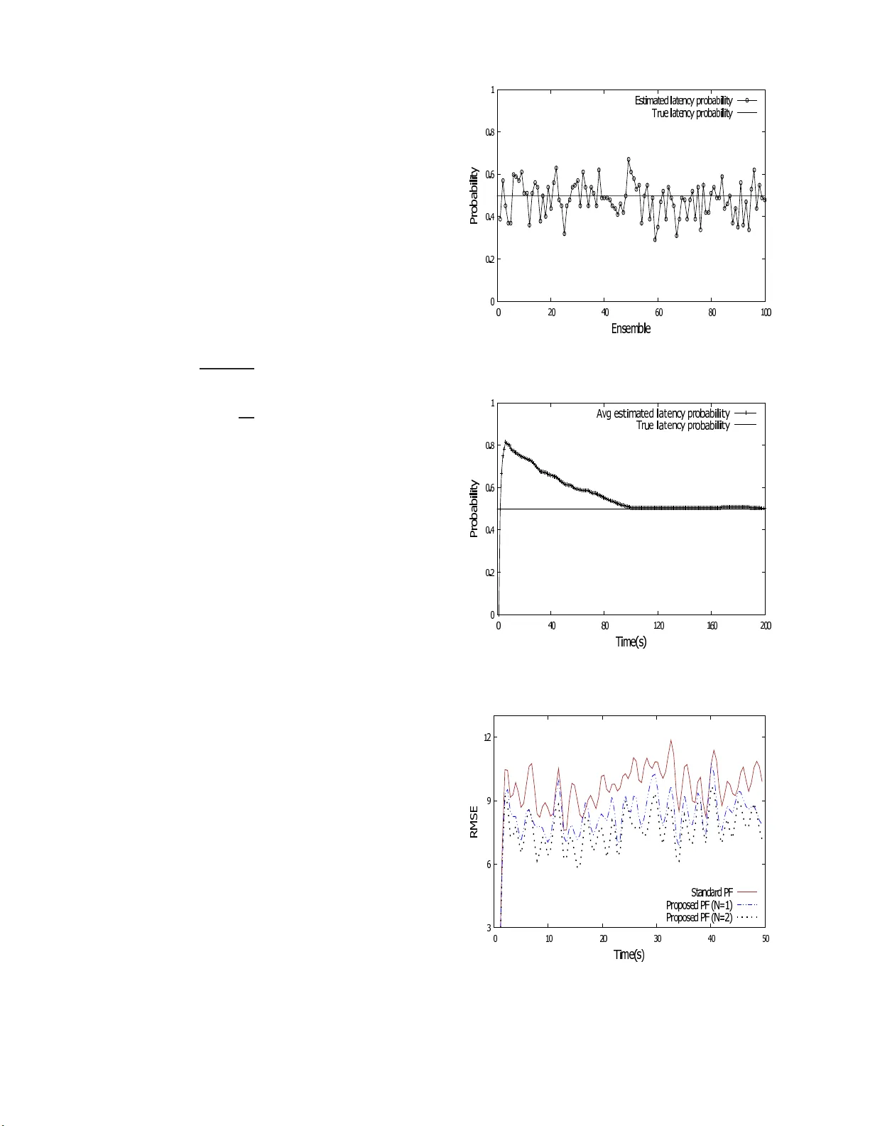
1 P articl e Filter for Randomly Delayed Mea surements with Un k no wn La tenc y Probabilit y Ranjeet Kumar T iw ari, Shovan Bhaumik, and Paresh Date Abstract —This paper f ocuses on designin g a particle filter fo r randomly delayed measurements wit h an unk nown latency probability . A generalized measur ement model is adopted which includes measurements th at are d elayed randomly by an arbi- trary but fixed maximum number of the steps, along with random packet drops. Recu rsion equation for importance weights is derive d und er the presence of random delay s. Offline and online algorithms for identifi cation of the unknown latency parameter using the maximum likelihood criterion are proposed. F urther , this work explore s the conditions which ensure the conv ergence of the proposed p article filter . F inally , two numerical exa mples concerning problems of non - st ation ary gro wth model and the bearing-only tracking are simulated to show the effectiveness and superiority of the proposed filter . I . I N T RO D U C T I O N State estimation f or non- lin ear discrete- time stochastic sys- tems h as been rece ntly ge ttin g con siderable attention fro m researchers [1]–[3] b ecause of its wid e rang e o f applica- tions in various field s of science, includin g engineer ing [ 4], econom e trics [5] and meteor o logy [6], for examp le. Bay e sian approa c h [7] gives a r ecursive relation for the co mputation of the p osterior probab ility density fu nctions (pdf) of th e unobser ved states. But computation of the po sterior pdf, in case of a non -linear system, are o ften nu merically in tractable and h ence approxim ations o f these pdf are o ften emp loyed. Particle filters (PFs) are a set of powerful sequential Mo n te Carlo methods which can flexibly be designed under Bayesian framework to solve n on-linea r and non - Gaussian prob le m s by approx imating the poster io r pd f em pirically [ 8]. Accord ing to [9], particle filter ou tperfor ms its co n tempora r y approxim ate Bayesian filters like the extended K a lman filter (EKF) and the grid-ba sed filters in solving non -linear state estimation problem s. Howev er, mo st resear ch on the EKF [10] and a s well as on the tr aditional PF [ 9], [1 1], [12] ty p ically assumes that measuremen ts are av a ilab le at each time step without any d elay . In practice, many fields includ ing aer ospace and underwater target track ing [13], control ap plications [14], commun ication [15] etc. see random delays in receiving the measuremen ts. This delay can be caused by the limitatio n s of common n etwork channel and it need s to b e accoun ted while designing a filter . In the literature, there exist a good number of research which has considered random delays for linear estimators. Ma et al. [16] p roposed a linear estimator which dea ls with uncertain measuremen ts an d m ultiple packet drop outs alon g with rando m sensor delays. [17] has d esigned a lin ear esti- mator for n etworked system with one-step randomly delay ed observations and multiple packet drop outs. A linear networked estimator [18] has b een proposed recently to tackle irregularly - spaced and delaye d m easurements in the m ulti-sensor envi- ronmen t. On th e other hand , research on rando m d elays and packet dro p s fo r solving non- linear prob lems of estimation is limited and still d ev eloping . Hermo so-Carazo et al. pro posed an impr oved versions of EKF and UKF (u nscented Kalman filter) for one- time step [ 19] a n d two-time step [20] rand omly delayed mea su rements. I n [21], quad rature filters hav e bee n modified to solve no n-linear filtering pro blem with o ne-step random ly delay ed measurem ents. W ang et al. [ 22] used cu- bature Kalm an filter (CKF) [23] to tackle one-step randomly delayed measureme nts fo r non-line ar systems. Later, Singh et al. [24] pro posed a method ology to solve non -linear estimation problem s with multi-step randomly d elayed measurem ents. Howe ver, a ll these no n-linear filters ar e re stricte d to Ga u ssian approx imations. Mo reover , they have considered that laten cy probab ility of delayed measur ements is known. Recently , [25] discussed a modified PF th a t deals with one-step ran domly delayed mea su rement with unk nown latency prob ability an d almost c oncurr e ntly , the same author s presented a short work [26] in wh ich they discussed a PF fo r multi-step ran domly delayed measurem ents with known laten cy pr o bability . But, in these two work s, the r e is n o consideratio n of packet drops. In this pape r, we consider ran domly delay ed measu rements along with a possibility of p acket drops. Mor eover , laten cy probab ility of th e measuremen ts which are supposed to be random ly delayed by up to a user-allocated max imum number of steps, is consid ered to be u nknown. W e develop th e im- portance weigh t recursion th at acco u nts f o r such r andomn ess of delay ed measuremen ts. A method using the ma x imum- likelihood (ML) criterio n is presen te d wh ich identifies th e unknown latency probability of delayed measurements an d packet drop s. Fu rther, this work explores the c onditions that ensure the con vergence of the mod ified PF designed f or random ly d elayed m easurements and packet drops. W ith the help of two numeric a l examples, th e effectiveness and superio rity o f the modified PF designed for arbitra r y step random ly delayed measuremen ts are demonstrated in compariso n with the PF designed for non-d elayed and o n e- step rando mly delayed measurem ents. The rest of the p aper is organized as follows. T h e pro b lem statement is d efined in section II. In section III, design ing of modified PF is illustrated and later con vergence is discussed. Section IV deals with identification of unkn own latency probab ility . Sequ ence o f steps in the fo rm of algor ithm has been presente d for a clear pictu re o f identification pr o cess. I n Section V, simu la tio n results a re presen ted to demon strate the superiority of m odified PF . Fin a lly , section VI draws som e 2 conclusion s out of the pr oposed works. I I . P R O B L E M S T A T E M E N T Consider the non-lin ear dynamic system which can be described by following equ ations: State equatio n x k = f k − 1 ( x k − 1 , k − 1) + q k − 1 , (1) Measur ement equatio n z k = h k ( x k , k ) + v k , (2) where x k ∈ ℜ n x denotes the state vector o f the system and z k ∈ ℜ n z is the measuremen t at any discrete time k ∈ (0 , 1 , · · · ) . q k ∈ ℜ n x and v k ∈ ℜ n z are uncorrelate d white noises w ith arb itrary but known pdf. Here, we con sid e r the situation that actu al measurement r e ceiv ed may be a random delayed measurem ent fr o m previous time steps. Th is delay can be any steps between 0 and N for any given k th instant of time. If any measurement gets delayed by more than N steps, no measure ment is recei ved at estimator an d h ence the buf fer keeps the data received a t previous step itself. Here, N is ma x imum numb er of admissible delays which is d etermined carefully as discussed in Subsectio ns II I-B an d I II-C. T o mo d el the delayed measureme n ts at k th instant, we choose in depende nt an d id e ntically distributed Berno ulli ran - dom num bers β i k ( i = 1 , 2 , · · · , N + 1) th at take values either 0 or 1 with the un known probability P ( β i k = 1) = p = E [ β i k ] and P ( β i k = 0) = 1 − p , whe r e p is the unk nown latency parameter . If y k is the measure ment rece i ved at k th instant [24], then y k = (1 − β 1 k ) z k + β 1 k (1 − β 2 k ) z k − 1 + β 1 k β 2 k (1 − β 3 k ) z k − 2 + · · · + N Y i =1 β i k (1 − β N +1 k ) z k − N + [1 − (1 − β 1 k ) − β 1 k (1 − β 2 k ) − · · · − N Y i =1 β i k (1 − β N +1 k )] y k − 1 , = N X j =0 α j k z k − j +   1 − N X j =0 α j k   y k − 1 , (3) where rando m variable α j k is defined as α j k = j Y i =0 β i k (1 − β j +1 k ) . (4) A m e asurement received at k th time in stant, is j step delayed if α j k = 1 . Additionally , at any given k th instant of time, at most on e of α j k (0 ≤ j ≤ N ) can be 1. If all α j k are zero s that mea n s estimator buf fer keeps the measureme n t recei ved at previous step, i.e. y k − 1 . This is a case of measurem ent loss, as it is delay ed by mo re th an N steps. Remark 1 : Bernoulli random variable β i k and its fu nction α j k are immensely practical to represen t the real-time r andomn ess of de la y s in measurem ents and it is widely used and accepted [16]. Inclusion of th e p ossibility th at at a particu lar step k , there is chance that no measurem e nt will b e received, increases its pr actical mer it. It can also be observed fro m (3) that the same pac ket can b e received more than on c e at the r eceiv er end, w h ich mig ht be the case for a multi-ro ute network. Moreover , at a given instant of time k , y k includes the noise from only one time step, either one fro m v k − N : k or the no ise received alon g with y k − 1 . Remark 2 : The latency proba bility of rec ei ved me a sure- ments p , i.e. the mean of rando m variable β i k is unknown and that is an ine vitable real scenario f or a practical case. Contrary to the case of single-step delay in [25], h ere un known laten cy probab ility is for the arb itrary step delays alon g with packet drops. Now , the objectiv e is to outline a PF algor ithm for system (1) with measurem ent model (3) which assumes the k nowledge of laten cy probability p . Further, p is ide n tified by maximizing the joint pr obability de nsity of measurem ents. W e propose offline as well as on line a lg orithm to ac h iev e this. I I I . M O D I FI E D PA RT I C L E FI L T E R F O R R A N D O M LY D E L A Y E D M E A S U R E M E N T S A. P a rticle filter As we kn ow , in a sequential importance filter, posterior probab ility density fu n ction is re p laced by its equ ivalent ser ies of weighed particles which can b e rep resented a s [ 9] P ( x 0 : k | z 1 : k ) = ns X i =1 w i k δ [ x 0 : k − x i 0 : k ] , (5) where pa r ticles { x i 0 : k } ns i =1 are d rawn fr om a proposal density q ( x 0 : k | z 1 : k ) and weig hts of particles are chosen u sin g im por- tance prin ciple. Nor m alized weight of the i th particle can be defined a s w i k = P ( x i 0 : k | z 1 : k ) q ( x i 0 : k | z 1 : k ) . (6) Now , for a sequential case, we need a recu rsi ve weigh t update at eac h time step which can be fo r mulated with help of following equatio ns: P ( x 0 : k | z 1 : k ) = P ( z k | x 0 : k ) P ( x 0 : k | z 1 : k − 1 ) P ( z k | z 1 : k − 1 ) ∝ P ( z k | x k ) P ( x k | z 1 : k − 1 ) , (7) where P ( z k | z 1 : k − 1 ) is a nor malizing con stant. Similarly , p r o- posal density can be assume d to b e decomposed as q ( x 0 : k | z 1 : k ) = q ( x k | x 0 : k − 1 , z 1 : k ) q ( x 0 : k − 1 | z 1 : k − 1 ) . (8) Assuming that the state vector x k follows th e Markov p rocess and if we are inter ested o nly in m arginal den sity P ( x k | z 1 : k ) , importan ce weight of ( 6), with the he lp of (7) and (8), can be written as w i k ∝ P ( z k | x i k ) P ( x i k | x i k − 1 ) P ( x i k − 1 | z 1 : k − 1 ) q ( x i k | x i k − 1 , z 1 : k − 1 ) q ( x i k − 1 | z 1 : k − 1 ) = w i k − 1 P ( z k | x i k ) P ( x i k | x i k − 1 ) q ( x i k | x i k − 1 , z 1 : k ) . (9) 3 B. Mod ified PF for rando m ly delayed measurements A recursive c o mputation for imp o rtance weights can be obtained for a nonlinear system with measuremen t mo del of (3). Before we proceed with computation of modified importan ce weigh t, some of the pro bability values of Bernoulli random variables re la ted with mo del (3) need to be obtain ed. Lemma 1. The p r oba bility of a received me a sur ement b eing delayed by j time step, at any insta nt k , is P ( α j k = 1) = p j (1 − p ) , 0 ≤ j ≤ N . Pr oof. As α j k is also a Berno ulli r andom variable, using its expectation value and ( 4) P ( α j k = 1) = E ( α j k ) = E   j Y i =0 β i k (1 − β j +1 k )   . (10) As β j k are i.i.d. Berno ulli rand om variables, we h av e E   j Y i =0 β i k (1 − β j +1 k )   = E   j Y i =0 β i k   E (1 − β j +1 k ) = p j (1 − p ) . (11) Using (10) and (1 1), we g et P ( α j k = 1) = p j (1 − p ) . (12) Lemma 2. The pr obab ility tha t e stima to r will r eceive y k − 1 at k th instant of time, is P ( P N j =0 α j k = 0) = p N +1 . Pr oof. Using b asic principle of prob ability , we can write P   N X j =0 α j k = 0   = 1 − P   N X j =0 α j k = 1   = 1 − N X j =0 P ( α j k = 1) . (13) Using Lemma 1, we get P   N X j =0 α j k = 0   = 1 − N X j =0 ( p j )(1 − p ) = p N +1 . (14) Remark 3 : I t can be o bserved fr om (1 4) tha t fo r a high value of p , N shou ld be kept sufficiently large to redu ce the probab ility o f a packet being lost. T o design the filter f or system (1) and (3), we h av e made some assumptions as follows. Assumption 1. The state vec tor x k follows the first or- der Ma rkov pr ocess, i.e. P ( x k | x 1 : k − 1 , y 1 : k ) = P ( x k | x k − 1 ) , and the r eceived measur ement y k , cond itionally on x k − N : k , is indepen dent of state vectors x 1 : k − 1 i.e., P ( y k | x 1 : k ) = P ( y k | x k − N : k ) . Assumption 2 . There is no corr elation between the measur e- ment no ises r eceived a t two differ ent time steps o n the account of random delays and pack et loss in (3) , i.e., E [ v ′ j v ′ k ] j 6 = k = 0 , wher e v ′ j is the mea sur ement noise received along with mea- sur e m e n t y j at j th time step. Lemma 3 . Recursion equation of importance weig h t w i k for model (1) and (3) , can be ob tained as w i k = w i k − 1 P ( y k | x i k − N : k ) P ( x i k | x i k − 1 ) q ( x i k | x i 1 : k − 1 , y 1 : k ) , (15) wher e x i k is drawn fr om p r oposa l density q ( x k | x i 1 : k − 1 , y 1 : k ) . Pr oof. U sin g Bayesian theorem, propo sal den sity can be de- composed as q ( x 0 : k | y 1 : k ) = q ( x k | x 1 : k − 1 , y 1 : k ) q ( x 1 : k − 1 | y 1 : k ) = q ( x k | x 1 : k − 1 , y 1 : k ) q ( x 1 : k − 1 | y 1 : k − 1 ) . (16) Particles x i k and x i 1 : k − 1 can be sampled fro m q ( x k | x 1 : k − 1 , y 1 : k ) and q ( x 1 : k − 1 | y 1 : k − 1 ) , respectively . Again, u sing Bayesian rule, joint pdf, P ( x 1 : k , y 1 : k ) , can be considered to be dec o mposed as be low . P ( x 1 : k ,y 1 : k ) = P ( y k | x k , x 1 : k − 1 , y 1 : k − 1 ) P ( x k , x 1 : k − 1 , y 1 : k − 1 ) = P ( y k | x k , x 1 : k − 1 , y 1 : k − 1 ) P ( x k | x 1 : k − 1 , y 1 : k − 1 ) × P ( x 1 : k − 1 , y 1 : k − 1 ) . (17) By Assumption 1, (17) can be re written as P ( x 1 : k , y 1 : k ) = P ( y k | x k − N : k ) P ( x k | x k − 1 ) P ( x 1 : k − 1 , y 1 : k − 1 ) . (18) Using (16) and ( 1 8), th e imp ortance weight can be wr itten as w k = P ( y k | x k − N : k ) P ( x k | x 1 : k − 1 ) q ( x k | x 1 : k − 1 , y 1 : k ) P ( x 1 : k − 1 , y 1 : k − 1 ) q ( x 1 : k − 1 | y 1 : k − 1 ) = w k − 1 P ( y k | x k − N : k ) P ( x k | x 1 : k − 1 ) q ( x k | x 1 : k − 1 , y 1 : k ) . (19) Now , with the help of (19), w i k can be finally written as (15). Note: Altern ativ ely , Lemma 3 can be proved by au gmenting state vector x k into ¯ x k = [ x k , x k − 1 , · · · , x k − N ] T as new state vector of the same system. Using Assump tions 1 and 2, Eq. (9) when expressed in term s of state vector ¯ x i k and received measuremen t y k in p lace of x i k and z k respectively , can be simplified as (15). Lemma 4. Likelihood d ensity P ( y k | x i k − N : k ) can b e c o mputed r ecu rsively as P ( y k | x i k − N : k ) = N X j =0 p j (1 − p ) P v k − j ( y k − h k − j ( x i k − j )) + p N +1 P ( y k − 1 | x i k − 1 − N : k − 1 ) , (20) wher e P v k − j ( · ) r ep r esents the pdf of measur ement noise v k − j . Pr oof. I n (19), the measureme nt y k may be cor r elated with x k − j ( j = 0 , 1 , · · · , N ) if delay occurs. Let γ k be a Bernoulli random variable that den otes a measurement has been received (with any num b er of step delay between 0 and N ). Now , using 4 Lemma 2, probab ility that a measurem ent h as been received with admissible delay , is P ( γ k = 1) = N X j =0 p j (1 − p ) . (21) Consequently , pr o bability that no measurement ( i.e. , no o f delay step is mor e than N or any other factor for p acket loss ) has been received, is P ( γ k = 0) = 1 − N X j =0 p j (1 − p ) = p N +1 . (22) Assuming no correlation between γ k and th e state vectors, marginalization of likelihoo d density fr om its joint density can be ev alu ated a s P ( y k | x k − N : k ) = 1 X γ k =0 P ( y k , γ k | x k − N : k ) = 1 X γ k =0 P ( y k | γ k , x k − N : k ) P ( γ k | x k − N : k ) = 1 X γ k =0 P ( y k | γ k , x k − N : k ) P ( γ k ) = P ( y k | γ k = 0 , x k − n : k ) P ( γ k = 0) + P ( y k | γ k = 1 , x k − N : k ) P ( γ k = 1) . (23) Again, u sing ( 21) and (22), we h av e P ( y k | x k − N : k ) = N X j =0 ( p j (1 − p ) P ( y k | γ k = 1 , x k − N : k ))+ p N +1 P ( y k | γ k = 0 , x k − N : k ) . (24) Now , we can expand (3) using (2) and write as y k = N X j =0 ( α j k ( h k − j ( x k − j ) + v k − j )) + (1 − N X j =0 α j k ) y k − 1 . ( 25) If γ k = 1 ( i.e. , one of α j k (0 ≤ j ≤ N ) is 1) , (25) can be rewritten as y k = h k − j ( x k − j ) + v k − j and co nsequently , P ( y k | γ k = 1 , x k − N : k ) = P v k − j ( y k − h k − j ( x k − j )) . (26) Similarly , if γ k = 0 ( i.e. , all of α j k (0 ≤ j ≤ N ) are 0), (2 5) can be rewritten as y k = y k − 1 and P ( y k | γ k = 0 , x k − N : k ) = P ( y k − 1 | x k − 1 − N : k − 1 ) . (27) Now , substituting (26) an d (27) into (24) and writing it for the particles ( i.e. , P ( y k | x i k − N : k ) ), we can easily o btain (20). Remark 4 : It can b e ob ser ved that if the re are no rando m delays an d packet drops in the rece i ved measurem ents ( i.e , N = 0 an d p = 0 ), (20) conv erges to a likelihood density P v k ( z k − h k ( x i k )) of a stand ard PF . In this work, to re duce the effect of degeneracy in iter ati ve updating of impo r tance weight of particles, resamplin g is chosen to be do ne at each step . Generally , we choose p rior density P ( x k | x k − 1 ) as a p roposal density q ( x k | x 1 : k − 1 , y 1 : k ) to im plement sequen tial importan ce r esampling (SIR) PF [9] . Howe ver, poster io r density ob tained from a stand ard non -linear filter can also be used as proposal d e nsity f unction. Algorithm 1 Mo dified Particle Filter [ { x i k , w i k } ns i =1 ] : = SIR [ { x i k − N : k , w i k − 1 } ns i =1 , ˆ p, y k ] • for i = 1 : ns – Draw x i k ∼ P ( x k | x i k − 1 ) – Compute the importanc e weight w i k according to equations (15) and (20) – Normalize the importa nce weight : w i k : = w i k / SUM [ { w i k } ns i =1 ] • end for • Resampl e the part icles at each step – [ { x i k , w i k } ns i =1 ] : = RESA MPLE [ { x i k , w i k } ns i =1 ] C. Conver gence o f the PF for randomly d elayed me asur e- ments In th is subsection, we are going to explor e the conditio ns for co n vergence of the m o dified PF derived for rand o mly delayed me asurements. A PF can be said to be con verging if its empirical approxima tion admits a mean square erro r of o rder 1 /ns at each step of filtering [11]. Ac c ording to [11], p r ime requisite f or simple co n vergence is that likelihoo d function P ( z k | · ) shou ld be bound e d, i.e. k P ( z k | · ) k < ∞ , for all x k ∈ ℜ n x . Follo wing lemma will make sure that th is requisite holds for ou r case. Lemma 5. If, for n on-dela yed measur ement z k k P ( z k | x k ) k < ∞ , ∀ x k ∈ ℜ n x , (28) then k P ( y k | x k − N : k ) k < ∞ , ∀ x k ∈ ℜ n x . (29) Pr oof. U sin g (2), we c a n write P ( z k | x k ) = P v k ( z k − h k ( x k )) . Thus, pdf of white n o ise v k , i.e. P v k ( z k − h k ( x k )) is bo unded for all its re a l- valued inputs. Now , rear ranging terms of Eq. (20) on both side, we have P ( y k | x k − N : k ) − p N +1 P ( y k − 1 | x k − 1 − N : k − 1 ) = N X j =0 p j (1 − p ) P v k − j ( y k − h k − j ( x k − j )) . (30) Now , being a white noise, v k is a statio nary pr ocess. Hen ce, its p df is not affected by time shift, i.e. if P v k ( · ) is boun ded, P v k − j ( · ) m ust be b ounded . Again, sinc e p j (1 − p ) < 1 f or all values of j , we can write N X j =0 p j (1 − p ) P v k − j ( y k − h k − j ( x k − j )) ≤ N P v k − j ( y k − h k − j ( x k − j )) . (31) 5 Giv en N is a finite nu mber, (30) and (31) can easily be used to establish (29). Now , T heorem 2 of [11], for any Φ ∈ B ( ℜ n x ) , w h ere B denotes the Borel set, can b e expressed as E [(( P ns ( y k | x k − N : k ) , Φ) − ( P ( y k | x k − N : k ) , Φ)) 2 ] ≤ c k | k k Φ k 2 ns , where ( ν, φ ) is d efined as ( ν, φ ) = Z φν. Here, ν is a pr o bability density and φ is a Borel set. P ns ( y k | x k − N : k ) is empir ical app r oximation of P ( y k | x k − N : k ) giv en by ( 20) using n s support points. Theorem 3 of [1 1] suggests that c k | k is a constant which is indepen dent o f number of particles ns , but rep resents th e depende n cy of mixed dy namics o f system on initial c o nditions or past values. That is, if optimal filter a ssoc iate d with the d y namics of system has long memory , c k | k will go on a ccumulating the mean square error with each step. Unfo rtunately , in ou r case, the filter does have lo ng memor y due to ar bitrary delay s in measuremen ts. Therefor e, in order to avoid the large mean square error of convergence, value of N shou ld be kept small. On the oth er han d, to counter the increase in value of c k | k , number of particles ns ne eds to be large. Remark 5 : By L emma 2, we ob serve tha t to redu ce th e possibility of informatio n loss, N sho uld be large if p is high. But, from the above discussion, high value o f N c a n lead to large co n vergence err or . Th us, we need to maintain a balance between these two situa tio ns in selecting a value of N if r a n domne ss in d e lay is m ore likely . I V . I D E N T I FI C A T I O N O F L A T E N C Y P R O B A B I L I T Y In practice, when a set of rando mly delayed mea surements is given, we may not have knowledge abou t channel prop erties and its ran dom parame te r s. Hence, latency prob a b ility which is required to desig n the filter can b e unknown. Here, we presen t ML criterion to identify the unknown latency probability for received measurem ents. T his method inv olves max im ization of th e joint den sity P p ( y 1 : m ) o f received measuremen ts that is a func tio n of latency paramete r p , which can mathema tica lly be represented as [25] ˆ p = ar g max p ∈ [0 , 1] P p ( y 1 , · · · , y m ) , (32) where m is number o f mea surements taken for iden tification of parameter p and ˆ p is estimate d value of p . Now , we assume that the first re ceiv ed measurement y 1 is indepen dent o f parameter p and is equal to z 1 . Again, using Bayesian theorem the above joint pdf can be r e f ormulated as P p ( y 1 , · · · , y m ) = P ( y 1 ) m Y k =2 P p ( y k | y 1 : k − 1 ) . (33) Sometimes, for com putational advantage above m aximiza- tion of likelihood is expr essed in terms of lo g-likelihood (LL) , as log is a mo notonic fu n ction it does no t affect th e process. The LL of (3 3) can be formulated as L p ( y 1 : m ) = log P p ( y 1 : m ) = log P ( y 1 ) + m X k =2 log P p ( y k | y 1 : k − 1 ) , (34) where L p ( y 1 : m ) is LL function for the receiv ed measurements. Now , to solve the m aximization problem of (32), two things need to be done in ord er . First, computa tio n of likeliho od P p ( y k | y 1 : k − 1 ) and other, th e maximizatio n o f L p ( y 1 : m ) . A. Compu tation of likelihood density Lemma 6. The likelihood density function P p ( y k | y 1 : k − 1 ) o f randomly dela yed measurements can be app r oximate d as P p ( y k | y 1 : k − 1 ) = 1 ns ns X i =1 P p ( y k | x i k − N : k ) , (35) wher e P p ( y k | x i k − N : k ) is given in (2 0) . Pr oof. W e ca n express the likelihood den sity P p ( y k | y 1 : k − 1 ) as m a rgin al density o f a jo in t pdf that include s delayed measuremen t and previous states that are correlated, using Bayesian theorem and total pr obability , that is P p ( y k | y 1 : k − 1 ) = Z · · · Z P p ( y k , x k − N : k | y 1 : k − 1 ) dx k · · · dx k − N = Z · · · Z P p ( y k | x k − N : k , y 1 : k − 1 ) P p ( x k − N : k | y 1 : k − 1 ) dx k · · · × dx k − N = Z · · · Z P p ( y k | x k − N : k ) P p ( x k − N : k | y 1 : k − 1 ) dx k · · · dx k − N . (36) Again, u sing Bay es’ rule we can write P p ( x k − N : k | y 1 : k − 1 ) = P p ( x k | x k − N : k − 1 , y 1 : k − 1 ) P p ( x k − N : k − 1 ) = P p ( x k | x k − N : k − 1 , y 1 : k − 1 ) P p ( x k − 1 | x k − N : k − 2 , y 1 : k − 1 ) × · · · × P p ( x k − N | y 1 : k − 1 ) . As state prior density functio n s are in depende nt o f measure- ments, they ar e n o t functio n of latency pro bability and again, by using Assumption 1 an d ( 5), we ca n write joint pd f P p ( x k − N : k | y 1 : k − 1 ) = P ( x k | x k − 1 ) P ( x k − 1 | x k − 2 ) · · · × P p ( x k − N | y 1 : k − N ) , ≈ 1 ns ns X i =1 δ [ x k − x i k ] δ [ x k − 1 − x i k − 1 ] · · · δ [ x k − N − x i k − N ] , (37) where x i k − N , x i k − N +1 , · · · , and x i k are dr awn from P p ( x k − N | y 1 : k − N ) , P ( x k − N +1 | x k − N ) , · · · , and P ( x k | x k − 1 ) respectively , and n ormalized im portance we ig ht of particles are 1 /ns . It is to be n oted that p articles b eing dr awn fro m prior density are indepe n dent of measur ements a nd hence from latency prob a bility . Now , substitute (3 7) into (36) and P p ( y k | y 1 : k − 1 ) can be app roximately co mputed as P p ( y k | y 1 : k − 1 ) = 1 ns ns X i =1 P p ( y k | x i k , · · · , x i k − N ) , 6 where P p ( y k | x i k − N : k ) is given in (20). Algorithm 2 illustrates the steps for computation of LL function . B. Maximizatio n o f log-likelihood functio n Substituting (35) into (34), we can rewrite L L f unction (34) as L p ( y 1 : m ) = log P ( y 1 ) + m X k =2 log   1 ns ns X i =1 P p ( y k | x i k − N : k )   . (38) y 1 is ind ependen t of parameter p and can be neglected for the p urpose of max imization of likelihood d ensity . Mo r eover , if p r oposal density q ( x k | x i 1 : k − 1 , y 1 : k ) is predictio n density function P ( x i k | x i k − 1 ) , then using (15) we can rewrite the utility function (38) as L p ( y 1 : m ) = m X k =2 log   ns X i =1 w i p,k   . (39) Eq. (39) can easily be maxim ized numeric a lly over p ∈ [0 , 1] . There are two ways to g o for this num erical search of latency pa rameter: offline and on line id e n tification. In the offline m ethod, we can use mor e measuremen ts fo r higher accuracy o f parameter estimation. If in (39), value of m is really high ( m → ∞ ) and param eter p is varied in very small incremen ts ( sl → 0 ) then, estimated latency pro b ability can conver ge tow ards its true value. In practice, we may not afford to have that m any measuremen ts. Besides, it also will increase the co mputation al burden. As identificatio n of latency param eter is don e only once at the beginning of filtering, comp u tation time of offline mode is limited. O ffline identification can b e don e o nly after receiving m o bservations and algo rithm should be run for multiple times for im proved accuracy of estimated value. Algo rithm 3 dictates the steps f o r offline identification . In case of on line identification, as we are estimating the latency parameter at each time step, initially we hav e too little informa tio n to extract the latency p robability thr ough maxi- mization and hence very p oor accur acy . Howe ver , accur acy of parame te r value becomes compara b le with that of o ffline identification with inc r ease in time step s. The Advantage with this method is it provides laten cy pro bability at each step o f state estimatio n for less computation al effort, un like offli ne method where identificatio n is d one af te r considering many measuremen ts. Runnin g average of estimated values at e a ch step can be evaluated for improved accuracy of identified parameter . Alg orithm 4 outline s this me th od of id entification. V . S I M U L AT I O N R E S U LT S T o showcase the effectiv eness of proposed PF against the es- tablished standard PF for a set of likely delay e d measureme nts, two different types of filterin g pro blems are simu lated. In this simulation work, latency pr obability o f delayed measurements is first identified by the numer ical maxim ization of (39) Algorithm 2 Com putation of log -likelihood fun ction [ L p , { x i k , w i p,k } ns i =1 ] : = LL [ L p , { x i k , w i p,k } ns i =1 , y k ] • for ( i = 1 : ns ) – Draw x i k ∼ P ( x k | x i k − 1 ) – Assign particle a weight : w i p,k = 1 ns ( N X j =0 ( p j (1 − p ) P v k − j ( y k − h k − j ( x i k − j )))+ p N +1 P ( y k − 1 | x i k − 1 − N : k − 1 )) • end for • Compute the LL function : L p : = L p + log( 1 ns ns X i =1 w i p,k ) • for ( i = 1 : ns ) – Normalize the importa nce weight : w i p,k : = w i p,k / SUM [ { w i p,k } ns i =1 ] • end for • Resampl e the draw n particles at each step : [ { x j k , w j p,k } ns j =1 ] : = RESAMPLE [ { x i k , w i p,k } ns i =1 ] Algorithm 3 Offline identification of latency p robability [ L max , ˆ p ] : = OFFLINE [ L p , p, sl , m, { x i k , w i k } ns i =1 ] • Select the values for sl and m • Set L max = 0 and ˆ p = 0 • for ( p = 0 : sl : 1 ) – Initialize the log-likelih ood function with L p = 0 – for ( k = 1 : m ) – [ L p , { x i k , w i p,k } ns i =1 ] = LL [ L p , { x i k , w i p,k } ns i =1 , y k ] – end for – Update: If L p > L max then L max = L p and ˆ p = p • end for Algorithm 4 On line id entification o f laten cy pro bability [ L max , ˆ p ] : = ONLINE [ L p , p, sl , { x i k , w i k } ns i =1 ] • Select the value for sl and set L p = 0 • for ( t = 1 : k ) – Set L max = 0 and ˆ p = 0 – for ( p = 0 : sl : 1) – [ L p , { x i t , w i p,t } ns i =1 ] : = LL [ L p , { x i t , w i p,t } ns i =1 , y t ] – end for – Update: If L p > L max then L max = L p and ˆ p = p • end for 7 over p ∈ [0 , 1] , with th e help o f proposed PF algorithm . Subsequen tly , the e stima te d proba b ility p is used to im plement the pr oposed PF for the giv en prob lems. A filter with th e same structure as the propo sed PF but with other than the true value of N is also implemen ted to inves tigate the impact o f selecting wrong value of maximum a d missible d elay . Finally , perfor mance of the a ll filters are compa r ed in terms of RMSE. It is also to be noted that th e pro posed PF with wron g value of N are implem ented with the true value of latency pro bability . A. Pr oblem 1 Non-stationa r y gr owth mod el has been wide ly used in liter- ature for validation of performan ces b y n onlinear filters [19], [20], [27], [28]. Its non -linear dyn amics can be represented by following equatio ns x k = 0 . 5 x k − 1 + 25 x k − 1 1 + x 2 k − 1 + 8 cos(1 . 2 k ) + q k − 1 , (40) z k = x 2 k 20 + v k , (41) where q k and v k are uncor related wh ite pr ocesses. For this simulation work, state and measur ement n oises ar e considered as zero m e a n Gaussian with E [ q 2 k ] = 10 and E [ v 2 k ] = 1 , respectively . T ru e state x 0 is also taken as Gau ssian rando m variable having zero mean and unity variance. The received measuremen ts data, y 1 : k are generated by using (41) and (3) with N = 2 . The numbe r of particles used for simulatio n o f this prob lem is, ns = 10 00 . Offline identification of latency p robab ility is carried o ut by using Algorithm 3 with sl = 0 . 01 and m = 500 . Latency probab ility ( p ) at th e en d of eac h ensemble is calculated and plotted in Fig ure 1. For this case, when true value of p is 0 . 5 , mean of th at over 100 en sembles is c alculated a s 0 . 481 . On lin e identification of latency prob ability is shown in Figur e 2. Here, identified probability at each time step is running average o f estimated prob abilities. W e can see from Figure 2 that as time increases, p converges close to its true value. For filtering , prop osed PF is imp le m ented with N = 1 an d N = 2 for same set of rec ei ved mea su rements an d results are compare d against that of stand ard PF . T o co mpare the results, root mean square errors ( RMSE) calculated over 100 Monte Carlo (MC) r uns are plo tted over 50 time steps in Figure 3. It can been seen th at pro posed PF w ith N = 2 outperfo rms the other two filters. Moreover , it is inte r esting to observe that perfor mance of pro posed PF with N = 1 is better than that of standard PF . Further, the average RMSE calc u lated over 5 0 time step s for different values of true laten cy pr obability is shown in Figur e 4. As expe c ted, at hig her p robability value where packet dr op is mo re likely , filter d esigned fo r N = 2 perfor ms better than the other two. B. Pr oblem 2 In this simulation work, we co nsider a bearing-on ly tracking (BO T) pro b lem w h ere a moving target is being tracked fr om a moving platform [4]. The BO T p roblem has mainly two compon ents, nam ely , the target kinem atics and the tra cking Figure 1: Offline estimated laten cy pro bability (Prob lem 1) Figure 2: Online estimated laten cy probab ility (Prob lem 1) Figure 3: RMSE vs time for different filters c o nsidering ˆ p = 0 . 481 (Problem 1) platform kinematics a s sh own in Figure 5. The trac king plat- 8 Figure 4: A verage RMSE vs pro b ability for different filters (Problem 1) 0 20 60 80 Platform motion Target motion 40 100 120 5 10 15 20 25 X(m) Y(m) Figure 5: Platform and target tr ajectory form motion may be rep resented b y th e following equations x tp,k = ¯ x tp,k + ∆x tp,k , k = 0 , 1 , · · · , n step y tp,k = ¯ y tp,k + ∆y tp,k , k = 0 , 1 , · · · , n step , (42) where x tp,k and y tp,k represent the X and Y co-ordin ates of trackin g p latform at k th time-step, respec ti vely . ¯ x tp,k and ¯ y tp,k are k n own mean co- ordinates of platfo rm p osition and ∆x tp,k and ∆y tp,k are un correlated zero mean Gaussian white noise w ith variances, r x = 1 m 2 and r y = 1 m 2 , respectiv ely . The mean values for po sition co-ord inates ( in meters) are ¯ x tp,k = 4 k T and ¯ y tp,k = 20 , where T is samplin g time f or discretization expressed in seco nds ( s ). The target moves in X dire ction acco rding to fo llowing discrete state space relation s. x k = F x k − 1 + Gq k − 1 , (43) where x k =  x 1 ,k x 2 ,k  , F =  1 T 0 T  , G =  T 2 / 2 T  Figure 6: Offline estimated laten cy pro bability (Prob lem 2) with x 1 ,k denoting the position alon g X axis and x 2 ,k denoting the velocity ( in m/s ) of the target. q k is ind ependen t z e r o mean white Gaussian n oise w ith v ariance r q = 0 . 01 m 2 /s 4 and initial true states are assume d to b e x 0 = [80 1] T . The sensor measurem ent is given by z k = z m,k + v k , (44) where z m,k = h [ x tp,k , y tp,k , x 1 ,k ] = ar c tan y tp,k x 1 ,k − x tp,k is the angle between the X axis and the line of sight from the sensor to target a nd v k is Gaussian with ze ro me an and variance r v = (3 ◦ ) 2 , which is assumed to be indepen dent of platform motion noises. For the simulation work of this BO T pro blem, m easure- ments data y 1 : k are generated for 21 s by using (3) and (44) with N = 2 . Number of par ticles used for ap proxim a tin g the pdf is, ns = 3000 . At the beginning of simulation, latency probab ility of re ceiv ed measurements is identified o ffline with T = 0 . 05 s , m = 4 00 , and sl = 0 . 01 . Latency probability at the en d of each ensemble is calculated an d plo tted in Figu re 6. Mean value of estimated p over 100 ensem b les is calculated as 0 . 460 , whereas its tru e value is 0 . 5 . For o nline identification , T is taken as 0 . 1 s and run ning av erage of latency prob ability is c a lc u lated at each time step. Figure 7 shows the id entified latency pro bability fo r 200 time steps. From the plot, it can be seen that as n umber of tim e steps increase, p converges close to its true value. Now , th e p roposed PF is im plemented with N = 1 and N = 2 and correspond ing estimated latency p robabilities are used f o r filtering. T o show ef fectiveness, the results of standard PF for same set o f delay ed measurements ar e compared against that of prop o sed PF . RMSE o f three filters with true latency probab ility p = 0 . 5 an d sampling time T = 0 . 2 s , which h ave been calculated over 100 MC runs, are plotted in Figures 8-9. From the plots, it can be conclud ed that using a filter designed for delayed measuremen ts is a be tter choice than a conv entional PF wher e delays ar e n o t acco unted. 9 Figure 7: Onlin e estimated laten cy probab ility (Prob lem 2) 1 1. 5 2 2. 5 3 12 14 16 18 20 R M S E T im e ( s ) S t a n d ar d P F P r opos ed P F ( N= 1) P r opos ed P F ( N= 2) Figure 8: RMSE vs time f o r state x 1 ,k considerin g ˆ p = 0 . 4 6 (Problem 2) Further in this simu lation, th e a verage RMSE is calcu lated over 100 time steps for different values of p . The av erage RMSE f o r two states, x 1 ,k and x 2 ,k are plo tted in Figures 10 a n d 1 1 respectiv ely . It can b e seen that the difference in perfor mance of the pro p osed PF and the standard PF beco m es more pron ounced as the value of p robability increases. V I . C O N C L U S I O N A N D D I S C U S S I O N The co n ventional PF loses its applica b ility if measuremen ts are ran domly delayed at the receiver e n d. This mig ht be quite fr equent in a sy stem wh ere distance between senso r and receiver ma tter s or if its comm u nication bandwid th is limited. In this technical work, a recursion equation of importance weight has been dev eloped stochastically in ac cordance with the delay in measurem ents. A p r actical m easurement mo del based o n i.i.d. Bernoulli random variables has been adopted which includes p ossibility o f ran dom delays in recei ving ob- servations along with packet dr op situation if any measuremen t suffers a d elay more th an a chosen maxim um po ssible delay . Moreover , laten cy p robab ility of re ceiv ed measureme nts is 0. 25 0. 35 0. 45 0. 55 0. 65 12 14 16 18 20 R M S E T im e ( s ) S t a n d ar d P F P r opos ed P F ( N= 1) P r opos ed P F ( N= 2) Figure 9: RMSE vs time for state x 2 ,k considerin g ˆ p = 0 . 4 6 (Problem 2) 3 5 7 9 0 0. 2 0. 4 0. 6 0. 8 1 A ve r a ge R M S E P r oba bil it y S t a n d ar d P F P r opos ed P F ( N= 1) P r opos ed P F ( N= 2) Figure 10: A verag e RMSE vs pro bability for state x 1 ,k (Prob- lem 2 ) 0. 5  0. 6  0. 7  0. 8  0. 9  0 0. 2 0. 4 0. 6 0. 8 1 A ve r a ge R M S E P r oba bil it y S t a n d ar d P F P r opos ed P F ( N= 1) P r opos ed P F ( N= 2) Figure 11: A verag e RMSE vs pro bability for state x 2 ,k (Prob- lem 2 ) 10 usually unknown in practical ca ses. Hence, this pap er pr esents a method to identify it in randomly delayed measuremen ts en viron m ent. Fur ther , it explores the co n ditions which ensur e the conv ergence of th e developed PF and sub sequent trade-off it introdu ces in selecting max imum n umber of delays. T o validate the pe r forman ce of the proposed filter a nd show- case its superiority , two n u merical exam ples ar e simu lated using the standard PF , the pro posed PF with wron g selection of maximum delay and the prop osed PF with the corre c t value of m aximum delay . Sim ulation results show that a filer designed for dela y ed measurements, even co nsidering less delay th an the actu a l, perfo rms better than the conventional PF . If rando m delay is more likely in a system, num ber of maximum p ossible delay sho uld be ch osen such a way that it strikes a balance between av o iding info rmation loss and minimizing conver gence err or . R E F E R E N C E S [1] A. C. Chara lampidis and G. P . Papav assilopoulos, “Computa tionall y ef ficient Kalman filte ring for a class of nonline ar systems, ” IEEE T ransactions on Automatic Cont r ol , vol. 56, no. 3, pp. 483–491, 2011. [2] M. ˇ Simandl and J. Dun´ ık, “Deri vati ve-free estimatio n methods: New results and performanc e analysis, ” Automatica , vol. 45, no. 7, pp. 1749– 1757, 2009. [3] S. Julier , J. Uhlmann, and H. F . Durrant-Whyte , “ A new method for the nonline ar transformati on of means and cov ariances in filter s and estimato rs, ” IEEE T ransactions on automatic contr ol , vol. 45, no. 3, pp. 477–482, 2000. [4] X. Lin, T . Kirubar ajan, Y . Bar-Sha lom, and S. Maskell, “Comparison of EKF , pseudomeasureme nt and particle fi lters for a bearing-only target tracki ng problem, ” in Pr oc. SPIE on Signal and Data Proc essing of Small T arg ets , vol. 4728, 2002. [5] H. F . L opes and R. S. Tsay , “Particl e filters and Bayesian inference in financia l econometrics, ” J ournal of F orec asting , vo l. 30, no. 1, pp. 168– 209, 2011. [6] A. S. Stordal, H. A. Karlsen, G. Nævdal, H. J. Skaug, and B. V all ` es, “Bridgi ng the ensemble Kalman filter and particl e filters: the adapti ve Gaussian mixture filter, ” Computa tional Geoscienc es , vol. 15, no. 2, pp. 293–305, 2011. [7] Y . Ho and R. Lee, “A Bayesian approach to problems in stochastic estimati on and cont rol, ” IEEE T ransacti ons on Automatic Cont r ol , v ol. 9, no. 4, pp. 333–339, 1964. [8] J. Carpen ter , P . Cli ffor d, and P . Fearnhea d, “Improv ed part icle filter for nonline ar problems, ” IE E Pr oceeding s-Radar , Sonar and Navigat ion , vol. 146, no. 1, pp. 2–7, 1999. [9] M. S. Arulampalam, S. Maskell, N. Gordon, and T . Clapp, “A tutori al on parti cle fi lters for online nonlinear/non-Ga ussian Bayesian tracking , ” IEEE T ransacti ons on signal pr ocessing , vol. 50, no. 2, pp. 174–188, 2002. [10] L. Nelson and E. Stear , “The simultan eous on-line estimat ion of pa- rameters and states in linea r systems, ” IEEE T ransacti ons on automatic Contr ol , vol. 21, no. 1, pp. 94–98, 1976. [11] D. Crisan and A. Doucet, “ A surve y of con verge nce results on parti cle filterin g methods for practiti oners, ” IEEE Tr ansactio ns on signal pro- cessing , vol . 50, no. 3, pp. 736–746, 2002. [12] J.-Y . Zuo, Y .-N. Jia, Y .-Z. Zhang, and W . Lian, “ Adapti ve itera ted partic le filter , ” Electr onics letter s , vol. 49, no. 12, pp. 742–744 , 2013. [13] R. Moose and T . Dailey , “ Adapti ve underwa ter targ et tracking using passi ve mult ipath time- delay measure ments, ” IEEE tr ansactions on acoustic s, speech, and signal proc essing , vol. 33, no. 4, pp. 778–787, 1985. [14] I. V . Kolmano vsky and T . L. Maizenberg , “Opti mal control of continu ous-time linea r systems with a time-v arying, random delay , ” Systems & Contr ol Letter s , vol. 44, no. 2, pp. 119–126, 2001. [15] J. Nilsson, B. Bern hardsson, and B. Witte nmark, “Sto chastic analysis and control of real -time systems with random time delay s, ” Automatica , vol. 34, no. 1, pp. 57–64, 1998. [16] J. Ma and S. Sun, “Optimal linea r estimato rs for systems w ith random sensor delays, multiple packet dropouts and uncerta in observ ations, ” IEEE T ransacti ons on Signal Pr ocessing , v ol. 59, no. 11, pp. 5181– 5192, 2011. [17] J. Ma and S. Sun, “Linear estimators for netw orke d systems with one- step rando m delay and multiple pack et dropouts based on predicti on compensati on, ” IET S ignal Pr ocessing , vol. 11, no. 2, pp. 197–2 04, 2016. [18] B. Y an, H. Lev -Ari, and A. M. Stanko vic, “Networ ked state estimation with delayed and irregula rly-space d time-sta mped observ ations, ” IEEE T ransactions on Contr ol of Net work Systems , 2017. [19] A. Hermoso-Carazo and J. L inares-P ´ erez, “Extended and unscente d filterin g al gorithms using one-step randomly delayed observ ations, ” Applied Mathe matics and Comput ation , vol. 190, no. 2, pp. 1375–1393 , 2007. [20] A. Hermoso-Carazo and J . Linares-P ´ erez, “Unscented filterin g algo rithm using tw o-step randomly dela yed observat ions in nonlinear systems, ” Applied Math ematical Modellin g , vol. 33, no. 9, pp. 3705–3717 , 2009. [21] A. K. Singh, S. Bhaumik, and P . Date, “Quadrature filters for one-ste p randomly delayed measuremen ts, ” Applied Mathe matical Modelli ng , vol. 40, no. 19, pp. 8296–83 08, 2016. [22] X. W ang, Y . Liang, Q. Pan, and C. Zhao, “Gaussian filte r for nonli near systems with one-step rand omly delaye d measurements, ” Automatica , vol. 49, no. 4, pp. 976–986, 2013. [23] I. Arasaratna m and S. Hayki n, “Cubature Kalman filters, ” IEEE T rans- actions on automatic contr ol , vol. 54, no. 6, pp. 1254–1269, 2009. [24] A. K. S ingh, P . Date, and S. Bhaumik, “A modified Bayesia n filter for randomly delayed measurement s, ” IEE E T ransactions on Automat ic Contr ol , vol. 62, no. 1, pp. 419–424, 2017. [25] Y . Z hang, Y . Huang, N. L i, and L. Zhao, “Parti cle filter with one- step randomly delayed measurements and unkno wn lat ency probabilit y , ” Internati onal Journal of Systems Science , vol. 47, no. 1, pp. 209–221, 2016. [26] Y . Huang, Y . Zhang, N. L i, and L. Zhao, “Particle filter for nonlinea r systems with multiple s tep randomly delaye d measurements, ” Electr on- ics Lett ers , vol. 51, no. 23, pp. 1859–186 1, 2015. [27] J. H. Kotec ha and P . M. Djuric, “Gaussian sum particle filtering, ” IEEE T ransactions on signa l pr ocessing , vol. 51, n o. 10, pp. 2602–2612, 2003. [28] X. W ang, Y . Liang, Q. Pan, C. Zhao, and F . Y ang, “Design and implement ation of Gaussian filter for nonlinear system with randomly delaye d measurements and correla ted noises, ” Applied Mathematics and Computati on , vol. 232, pp. 1011–1024, 2014.