Polarization and Index Modulations: a Theoretical and Practical Perspective

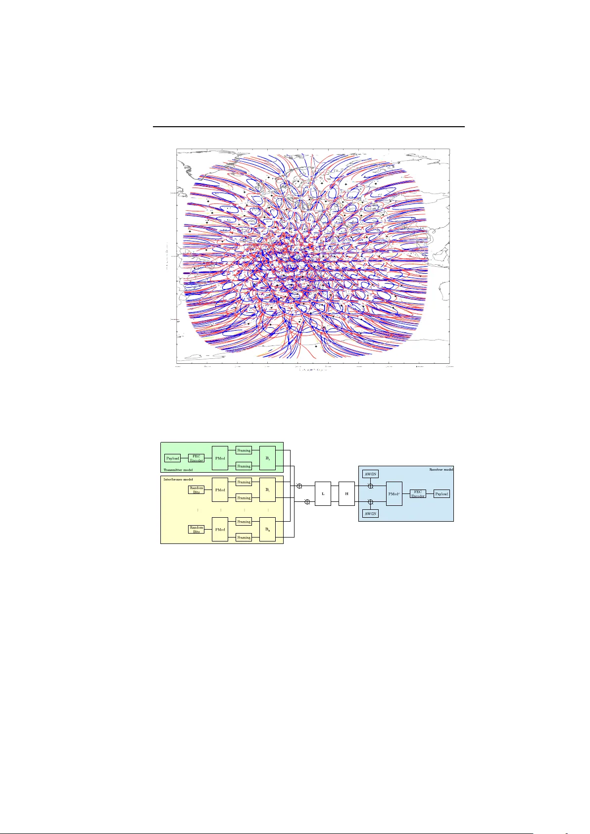
U N I V E R S I TAT P O L I T ` E C N I C A D E C ATA L U N YA D O C T O R A L T H E S I S Polarizat ion and Index Modulation s: a Theoretic al and Practical Pers pective by P O L H E N A R E J O S Dir ector: Prof. Ana Isabel P ´ E R E Z - N E I R A A thesi s subm itted in fulﬁlment of the requir ements for the degr ee of D O C T O R O F P H I L O S O P H Y in the Departament de la T eoria del Senyal i Comunicaci ons in collaboration w ith Centre T ecnol ` ogic de T elecomunicacions d e Catalunya Barc elona, June 1, 2017 iii “ My great est concern was what to call it. I thought of calling it infor - mation, but the word w as overly used, so I decided to call it un certainty . When I discussed it with Joh n von Neum ann, he had a better idea. V on Neumann told me, ≪ Y o u should call it entr opy , for tw o r easons. In the ﬁrst place your uncertai nty fu n ction has been used in statis tical m echa- nics under that name, so it alrea dy ha s a name. In the second place, and mor e important, nobody knows what entr opy rea lly is, so in a debate you will always hav e the advantage. ≫ ” Claude Elwood Shannon (1916—200 1) v Universitat Po lit ` ecnica de Catalunya Abstract Departament d e la T eoria del Se nyal i Comunicacions Centre T ecnol ` ogic de T elecomunicacions d e Catalunya Doctor o f Philosophy Polarization and Ind ex Mo dulations: a Th eoretica l and Practica l Pers pective by Pol H E N A R E J O S Radiocommunication s ystems have evolv ed s igniﬁcantly in r e- cent years in order to meet present and future demands. His- torically , time, fr e quency and mor e recently , spatial dimensions have been used to impr ove capacity and robustness . Paradoxi- cally , radiocommunications that leverage the po lariza tion d imen- sion have no t evolved at the same pace. In particul ar , the se com- munications ar e widely use d by satellites, w here several s treams ar e multiplexed in each orthogon al polarization. Curr ent communication trends advocate for simplifying and unifying dif fer ent frameworks in or der to incr ease ﬂexibility and address future needs . Due to this, sys t ems that d o not r e quire channel information are p rogr e ssively g aining traction, as t hey help to impr ove the overall quality of the network inst ead of t h at of speciﬁc users only . The search for new paradigms aimed at improving the quality of wir eles s communica tions is unstoppable. In or der to increase the capacity of current communications systems, new horizons and physical dimensions must be ex p lored. This disser t ation ai ms at challenging this perspe ctive and pr o- moting the us e of polarization in ne w radiocommunication sys- tems. Consequ ently , the goal of this the sis is tw ofold: ﬁrs t, w e vi aim at increasing the current capaci ty o f point-to-point and point- to-multipoint links. Se condly , we intr oduce new mechani sms to incr ease the robustness o f communications in particularly hostile envir onments. In this context, this thesis advocates for the us e of polarization as a dimension to be exploited in radiocommunicati- ons. In add ition to the us e o f polarization, index modulations he lp incr ease transmission rates w h ilst improving robustnes s against errors and imperfections with a low compu t ational complexity . Thus, the s tudy of polarization in these s ystems is esse ntial. This dissertation explores primordia l aspects in this ar ea, such as chan- nel capacity , transmitter and receiver design and performance ben- chmarking with current sys tems. F inally , w e ide ntify and discus s various characteristic aspects of p olarization. In this thesis, the reader w ill navigate the mathematical foun- dations o f the p roposed concep ts as well as their implement ation in r eal-life scenarios. After all , engineering excels at the inter- section of the u n d erlying physical principles with their real-l ife implementation. vii Universitat Po lit ` ecnica de Catalunya Resum Departament d e la T e oria del Senyal i Comunicacions Centre T ecnol ` ogic de T elecomunicacions d e Catalunya Doctor o f Philosophy Polarization and Ind ex Mo dulations: a Th eoretica l and Practica l Pers pective by Pol H E N A R E J O S Els sist emes de radiocomunicaci ons han e volucionat signiﬁcativa- ment els ´ ultims anys per cobrir les exigents demandes del present i el futur . Hist ` oricament s’han u tilitzat les dimensions temporal i freq ¨ uencia l, i m ´ es recentment la e s pacial, per do tar les radio- comunicaci ons d e m ´ es capac itat i robustesa. Paradoxalment, les radiocomunicaci ons que utilizen la dimens i ´ o d e polaritzaci ´ o no han evolucionat al mateix ritme. Concr etament, s’utilitzen sig- niﬁcativa ment en r adiocomunicacions per sat ` el · lit, multiplexant canals en cada polari tzaci ´ o o rtogonal. Addicionalment, la tend ` encia actual ´ es la de s impliﬁcar i uni- ﬁcar diferents mar cs de treball per ﬂexibilitzar i millorar les adap- tacions a les futures necessitats. Per aquesta ra ´ o, els s istemes r o- bustos que no requereixen informac i ´ o de canal es tan guanyant im- port ` ancia , ja que aj uden a millorar la qu alitat global de la xarxa i no nom ´ es per a determinats u s uaris. La cerca de no us paradigmes que milloren la qualitat de les comunicaci ons inal ` amb riques ´ es constant i imparable. Per aquesta ra ´ o es fa necessari buscar nous horitzons i noves d imensions f ´ ısiques que pe rmetin incrementar la capacitat actual de les comunicaci- ons. viii La present dissertaci ´ o vol canviar aquest a perspectiva i poten- ciar l’ ´ us de la polaritza ci ´ o e n els no us s istemes de radiocomuni- cacions. L ’objectiu d’aquesta tesi do ctoral ´ es doble: primer , in- cr ementar la capacitat actual dels enllac ¸ os punt a punt i punt a multipunt i, s e gon, do tar- los de millor r o bustesa davant d’entorns hostils. Per ai x ` o, aque s ta te si presenta la polaritzaci ´ o com a una dimensi ´ o a e xplotar e n les radiocomunicacions. Paral · lela ment, les modulacions per ´ ındex incr ement en la velo- citat d e transmissi ´ o, alhora que p ropor cionen una major robus- tesa davant errors i imperfeccions, tot mantenint una bai xa com- plexitat computacional. Aix´ ı doncs, l’est udi de la polaritzaci ´ o en aquests sistemes es fa necessari i primor dial. El present ma nuscrit estudia aspe ctes com la capacitat de canal en aquest s ` ambits, el seu disseny tant del transmissor com del r eceptor , aix ´ ı com com- paracions amb sistemes ex ist ents. Finalment, tamb ´ e s’analitzen diferents aspectes caracter ´ ıstics i ´ unics de la polaritzac i ´ o i es pr o- posa una nova modulaci ´ o en 3 dimensions , ´ unicament pos sible utilitzant la polaritzaci ´ o. En aquesta dissertaci ´ o el lector podr ` a trobar els fonaments ma- tem ` atic s que sustenten e l que es presenta aix´ ı com implementaci- ons r ealistes de les d iferents propostes e n entorns reals. L ’ ` exit de l’enginyeria es produeix quan s’aconseg ueix amalgamar els fon a- ments te ` orics amb la implementabilitat e n entorns reals. ix Universitat Po lit ` ecnica de Catalunya Resumen Departament d e la T e oria del Senyal i Comunicacions Centre T ecnol ` ogic de T elecomunicacions d e Catalunya Doctor o f Philosophy Polarization and Ind ex Mo dulations: a Th eoretica l and Practica l Pers pective by Pol H E N A R E J O S Los sistemas de r adiocomunicaciones han evolucionado signiﬁca- tivamente en los ´ ultimos a ˜ nos para cubrir las exigent es deman- das d el presente y el futuro. Hist ´ oricamente se han utilizado la s dimensiones tempo ral y frecuencial, y m ´ as recientemente la es- pacial, para dotar las radiocomunicaciones d e m ´ as capacidad y robustez. Parad ´ ojicamente, las radiocomunica ciones que utiliz an la dimens i ´ on de la polarizaci ´ on no han e volucionado al mismo ritmo. Concr etamente, se ut iliza n signiﬁcativamente en enlaces con sat ´ elites, multiplexando ca nales en cada polariz aci ´ on ortogo - nal. Adicionalmente, la te ndencia actual es la de s impliﬁcar y uni- ﬁcar diferentes mar cos de trabajo para ﬂexibilizar y mejorar las adaptaciones a las fut uras ne cesidades. Por esta raz ´ on, los sis- temas r obustos que no requieren informaci ´ on de canal est ´ an ga- nando importancia, ya qu e ayud an a mejorar la calidad global d e la red y no s ´ olo para det e rminados usuarios. La b ´ usqueda de nue vos paradigmas que mejoran la calidad de las comunicaciones inal ´ am bricas es const ante e imparable. P o r este mot ivo s e hace necesario buscar nuevos ho rizontes y nuevas dimensiones f ´ ısicas que permitan inc rementar la capac idad actual de las comunicaciones. x La pr esent e disertaci ´ on quiere cambia r es ta perspectiva y po- tenciar el uso de la p olarizac i ´ on en los nuevos sistemas de radi- ocomunicaciones. E l objetivo de esta tesis doctoral es doble: pri- mero, incrementar la velocidad de transmisi ´ o n actual de los en- laces punt o a punto y punto a multipunt o y , segundo, dotarlos de una mayor robustez e n entorno s hostiles. Por ello, esta t esis presenta la polarizaci ´ on como una dimensi ´ on a ex p lotar en las ra- diocomunicaciones. Paralelamente, las mod u laciones por ´ ındice incr ementan las velocidades de tr ans misi ´ on, a la par que proporcionan una ma- yor r obustez ante e r rores e imperfecciones, logrando mantener la complejidad comp u tacional baja en todo momento. As´ ı pue s, el estu d io de la polariza ci ´ on en est os sistemas se hace necesario y primordial . El presente manuscrito est udia aspecto s como la capacidad de canal en e stos ´ ambitos, su dise ˜ no t anto del t r ans - misor como del receptor , as´ ı como comparaciones con sist emas existente s. F inalmente, tambi ´ en se analiza n difer e ntes aspectos caracter ´ ısticos y ´ unicos de la polarizaci ´ on y se propone una nu- eva mo d ulaci ´ on en 3 dimensione s, ´ unicamente posible utilizando la polarizaci ´ on. En esta dise rtaci ´ on el lector podr ´ a encontrar los fundamen- tos matem ´ aticos que suste ntan lo que se presenta, as´ ı como im- plementaciones realistas de las distintas propuestas en ento rnos real es. El ´ e xito de la ingenier´ ıa se produce cuando se consigue amalgama r los fundamentos te ´ oricos con la implementabil idad e n entornos reales. xi Pr eface This the sis o riginates from the curiosity driving an e ngineer to discover new ways t o improve current communication sys tems in his spare time. Jugg ling work, family and pers onal pass ions is not always an easy task. Contrary to the common belief, the key ingredient of a doctoral the s is is no t te chnical k n o wledge n o r academic s kills, but a high degree o f perseverance and patience. Conducting s cience is no t always a grateful task. Experiments sometimes do no t turn ou t as expected and this, in turn, r esults on contradictions t hat can e asily infuse a se nse of defeat. In very few occasions, unique discoveries ar e made - revolutions that t ruly have an impact on the world as we k now it. However , the vast majority of expe riment out comes often fail to provi de an answer to t he very qu e stions t hey se ek to address. T rue science is based p reci sely on this premise: to depart from personal beliefs in order to ﬁnd objective, evidence-based truths . One of the s ituations t h at made a particular im pact in my pr ofes- sional career was when a student knocked on the door of a retir ed professor and showed him the results of an experiment based on a theory in which he had work e d all his life. The exp eriment actu- ally pr o ved the existence of his theory . Wh at I found particularl y impr essive was no t the magnitude of t h e discovery , but th e fact that he was able to de tach himself from his feelings and follow the path of s cience, although that meant departing from his per- sonal beliefs. W ith mo d esty and humility , this thesis aims at providing a small contribution t o the ﬁe ld of communications by polariza- tion. I still remember when I ﬁrs t heard the word po larization. I was twelve when my mother bought a parabolic antenna and a receiv er as a gift to watch foreign TV cha nnels. What stroke me the most was that two dif fer ent channels could us e the same fr e- quency simultaneously just by changing t heir polarization. Who xii would have th o ught that 20 y ears later I wou ld be writing my do c- toral thesis on communication syst e ms built upo n the very same concept of polarization. This t hesis only bears my n ame but it would not have bee n possible without the contribution of many other people who have contributed with their point of vi ew . From gr eat discussions, te chni- cal ar guments, ideas and informal talks this dissert ation has ﬁ- nally emer ged. Therefore, this thesis al so serves as tes timony of gratitude to the cou n t less contributions from many dif ferent pe- ople. The ﬁrst acknowledgement is for my family . My wife, Sara, has been th e main breadwinner during all t hese y e ars. Thanks to her love, patience and understanding this thesis has ﬁnall y be en able t o se e the light. And to my children, Lluc and Mateu, fo r being the best t h ing that has ever happened to me. The second thanks go to my p ar ents, ` Angels and ` Angel. Edu- cating a child comes with a great r espons ibility and this is not always easy . Thanks to them I am who I am. F rom them I have le- arned to take r esponsibility for my commitments and to have tr ue determination and grit. And , espe cially , my mot her , beca use her unconditional love has taught me t o love e verything I do. The thir d thanks goes to my thes is director , Ana. W e met 10 years ago while I was still ﬁnishing my university stud ies. S h e saw somet hing in me and from that moment we began to work togeth e r . Thanks to her I discovered the world of academic rese- ar ch and that the bes t w ay to achieve my objectives is to never stop perse vering. I would also li ke to extend a huge thanks to my gr e at friend, Jaume. Not o nly have we s p ent countless hours discuss ing about fascinating to pics, but we have also helped each ot h e r in many occasions. A lso , I would like to express my sp ecial gratitude fo r helping me carry out the ar duous t ask o f reviewing this thesis. Finally , I would li ke to t h ank all my colleagues at the Centre T ecnol ` o g ic de T elecomunicacions de Catalunya for being not only xiii rema rkable human beings, but also extremely competent professi- onals. Y o u make work ing here a fantastic exp e rience. In addition, I would also like to thank its entire management boar d for allo- wing me to p ursue this thesis and help me to combine my profes- sional o bligations w ith this d ivertimento. And lastly , I also want to thank you, reader , for showing in- terest and apprecia tion in t he work that I her e by present. I hope you ﬁnd it u seful and he lpful. xv Contents Abstract(e nglish, catalan and spanish) v Preface xi 1 Introduction 1 1.1 Presentation, Motivation and Objectives . . . . . . . 1 1.2 Structure of the Dissert ation . . . . . . . . . . . . . . 2 2 State of the Art and Fund amentals 9 2.1 Communication S ystems withou t CSI . . . . . . . . 9 2.1.1 Orthogonal B lock Code s . . . . . . . . . . . . 15 Other B lock Code s . . . . . . . . . . . . . . . 17 2.1.2 Data Multiplexing . . . . . . . . . . . . . . . 18 2.1.3 Index Mo d ulations . . . . . . . . . . . . . . . 19 Applications to Spatial Dimension . . . . . . 21 Applications to Frequency Dimension . . . . 23 Applications to Polarization Dimension . . . 23 2.2 Polarization as a N atural Diagonalizer . . . . . . . . 24 2.3 Fundamentals of Electromagnetic Polarization . . . 27 2.3.1 Stokes V ector . . . . . . . . . . . . . . . . . . 29 2.3.2 Reference System . . . . . . . . . . . . . . . . 31 2.3.3 Common Polarizations . . . . . . . . . . . . . 31 2.3.4 Reﬂection on S u rfaces: Specular Component 36 2.3.5 Faraday Effect . . . . . . . . . . . . . . . . . . 38 2.4 Polarization in In d ex Modu lations Implement ation 39 2.4.1 Speciﬁc Polarizations . . . . . . . . . . . . . . 40 2.4.2 Dual Polarized A ntennas . . . . . . . . . . . 41 xvi 3 Capacity An alysis of Ind ex Mod ulations 45 3.1 System Model and Capacity . . . . . . . . . . . . . . 46 3.1.1 Capacity analysis in high S NR . . . . . . . . 53 3.2 Remainder A nalysis . . . . . . . . . . . . . . . . . . 53 3.3 Ergodic Capacity . . . . . . . . . . . . . . . . . . . . 55 3.4 Results . . . . . . . . . . . . . . . . . . . . . . . . . . 56 3.4.1 Analytical R e sults . . . . . . . . . . . . . . . 57 3.4.2 Applications of In d ex Modu lations . . . . . . 60 Spatial Mod ulation . . . . . . . . . . . . . . . 61 Polarized Mo dulation . . . . . . . . . . . . . 63 Frequency Index Mo dulation . . . . . . . . . 65 3.5 Conclusions . . . . . . . . . . . . . . . . . . . . . . . 67 4 Polarized Mod ulation 69 4.1 System Model . . . . . . . . . . . . . . . . . . . . . . 70 4.2 Demodulation Scheme s . . . . . . . . . . . . . . . . 72 4.2.1 Optimal R eceiver . . . . . . . . . . . . . . . . 72 4.2.2 Suboptimal R eceivers . . . . . . . . . . . . . 73 Linear Re ceiver . . . . . . . . . . . . . . . . . 74 Likelihood Ratio with Hard Decision . . . . 75 Likelihood Ratio with Soft Decision . . . . . 76 4.3 Numerical Re sults for Uncod ed BE R . . . . . . . . . 78 4.3.1 Equal SE A nalysis . . . . . . . . . . . . . . . 82 4.4 Results in a Re alistic Sys t em Context . . . . . . . . . 83 4.4.1 Next Ge n e ration S atellite Communications Simulation Framewo rk . . . . . . . . . . . . . 84 4.4.2 Comparing PMod Solutions . . . . . . . . . . 90 4.4.3 Comparing PMod SD with Other Solutions . 91 4.4.4 XPD Analysis . . . . . . . . . . . . . . . . . . 92 4.4.5 Imperfect Channel E stimation . . . . . . . . 95 4.5 Conclusions . . . . . . . . . . . . . . . . . . . . . . . 97 5 3D Polarized Mod ulation 99 5.1 Sphere Modulation . . . . . . . . . . . . . . . . . . . 99 5.2 Enabling Po larized Mod ulation . . . . . . . . . . . . 103 xvii 5.2.1 Joint Re ce iver . . . . . . . . . . . . . . . . . . 105 5.2.2 Cascade R eceiver . . . . . . . . . . . . . . . . 106 5.3 BER Analysis . . . . . . . . . . . . . . . . . . . . . . 107 5.4 Results . . . . . . . . . . . . . . . . . . . . . . . . . . 116 5.4.1 Comparison of Classes of Re ce ivers . . . . . 119 5.4.2 Comparison of Differ e n t Modulation Orders 120 5.4.3 Comparison with Othe r Exist ing Scheme s . . 120 Comparison with 2D PMod . . . . . . . . . . 121 5.5 Conclusions . . . . . . . . . . . . . . . . . . . . . . . 122 6 Adaptive Modulation, Coding and M IMO Schemes w ith Dual Po lariza tion 131 6.1 PHY Layer Abst r action (PLA ) . . . . . . . . . . . . . 132 6.2 PLA and MIMO . . . . . . . . . . . . . . . . . . . . . 135 6.2.1 RBIR for ML Re ceivers . . . . . . . . . . . . . 136 6.2.2 RBIR for L inear Rece ivers . . . . . . . . . . . 138 SISO . . . . . . . . . . . . . . . . . . . . . . . 138 Orthogonal Po lariza tion T ime Block Codes . 138 Polarization Mu ltiplexing . . . . . . . . . . . 138 Polarized Mo dulation . . . . . . . . . . . . . 139 6.3 Adaptive MODCOD and MIMO Scheme . . . . . . 139 6.4 Channel T ime Se ries Generator . . . . . . . . . . . . 140 6.4.1 Mobile Satellite Dual Polarized Channel Mo- del . . . . . . . . . . . . . . . . . . . . . . . . 141 6.4.2 Interference Model . . . . . . . . . . . . . . . 143 6.5 Remarks . . . . . . . . . . . . . . . . . . . . . . . . . 145 6.6 Results . . . . . . . . . . . . . . . . . . . . . . . . . . 146 SISO Sce n ario: the ben chmark . . . . . . . . 146 Fixed MIMO: th e ot her benchmark . . . . . . 147 MIMO Scenario: full adaptation . . . . . . . 149 6.7 Conclusions . . . . . . . . . . . . . . . . . . . . . . . 154 7 Final 157 7.1 Conclusions . . . . . . . . . . . . . . . . . . . . . . . 157 7.2 Future Research . . . . . . . . . . . . . . . . . . . . . 161 xviii 7.2.1 QAM & 3D PMo d . . . . . . . . . . . . . . . 161 Constant Radius I s sue . . . . . . . . . . . . . 161 Maximizi ng the Distance . . . . . . . . . . . 162 7.2.2 Orbital An g ular Mo mentum Modulations . 164 OAM Generation . . . . . . . . . . . . . . . . 165 Beamforming and OAM . . . . . . . . . . . . 170 A Decoupling Linear Po lariza tions 171 B Linear Block Codes 175 B.1 Orthogonal Block Cod es . . . . . . . . . . . . . . . . 175 B.2 Data Mu ltiplexing . . . . . . . . . . . . . . . . . . . . 176 B.3 Other Block Cod es . . . . . . . . . . . . . . . . . . . 177 C Demonstration of F araday Effect 179 C.1 W ave N u mber Analysis . . . . . . . . . . . . . . . . 183 D Derivations o f the E rgodic C apacity 187 D.1 Nakagami- m Channel . . . . . . . . . . . . . . . . . 187 D.2 Rice Channel . . . . . . . . . . . . . . . . . . . . . . . 189 E CASTLE : the Platform where Researchers can Develop Standards 191 E.1 Architectur e . . . . . . . . . . . . . . . . . . . . . . . 195 E.2 Handshaking & Session . . . . . . . . . . . . . . . . 197 E.3 Licensing . . . . . . . . . . . . . . . . . . . . . . . . . 198 F Bro adb and Global Area Network Standard 201 G Proofs of Theorems (1) and (2) 203 H Reference T ables 209 Bibliography 213 xix List of Figures 2.1 Index Mo d ulation Diagram. . . . . . . . . . . . . . . 20 2.2 Index Mo d ulation Diagram. . . . . . . . . . . . . . . 26 2.3 Electric ﬁeld of horizontal and vertical polarizati- ons for a particular time instant. . . . . . . . . . . . . 32 2.4 Electric ﬁeld of 45 ◦ slant polarization for a particu- lar time inst ant. . . . . . . . . . . . . . . . . . . . . . 36 2.5 Electric ﬁeld of − 45 ◦ slant polarization for a parti- cular time instant. . . . . . . . . . . . . . . . . . . . . 36 2.6 Electric ﬁe ld of R H CP for a particular time instant. . 37 2.7 Electric ﬁe ld of L HCP for a particular time instant. . 37 2.8 Cir cular polarization antennas. . . . . . . . . . . . . 41 2.9 Dual polarized antennas. . . . . . . . . . . . . . . . . 42 2.10 Septu m polarizer . . . . . . . . . . . . . . . . . . . . . 43 3.1 A verage instantaneous capaci ty appr oximations for dif ferent orders compared to the integral-based ex- pression for N t = 2 and N r = 2 . . . . . . . . . . . . . 58 3.2 Normalized error of the dif ferent approximation or- ders for N t = 2 and N r = 2 . . . . . . . . . . . . . . . 59 3.3 Approximations of the capacity for differ ent orders compar ed to the upper and lower bou n d s descri- bed in [ RHH14 ]. . . . . . . . . . . . . . . . . . . . . . 60 3.4 Capacity evaluation for differ ent ante nnas at trans- mission and r eception applying IM t o the spatial domain of L TE ETU cha nnel for low and high an- tenna correlations. . . . . . . . . . . . . . . . . . . . . 63 xx 3.5 Capacity evaluation for differ e n t scenarios applying IM t o t h e polarization domain of Land Mobile Sa- tellite channel. . . . . . . . . . . . . . . . . . . . . . . 64 3.6 Snapshot o f the spe ctrum of the ETU channel model. 66 3.7 Capacity evaluation for s everal frequency separa- tions applying IM to the fr equency domain of L TE ETU channel. . . . . . . . . . . . . . . . . . . . . . . 67 4.1 Reception scheme. PMod − 1 applies one of th e fol- lowing de modulation s chemes to est imate the bit l . 73 4.2 Reception scheme. PMod − 1 applies the approach described in this s ection. . . . . . . . . . . . . . . . . 77 4.3 Comparison of the uncoded BER of the four propo- sed PMod techniques conveying a QPSK conste lla- tion. . . . . . . . . . . . . . . . . . . . . . . . . . . . . 80 4.4 Comparison of the uncode d BER of the PMod SD with o ther existing techniques conveying a QPSK constellation. . . . . . . . . . . . . . . . . . . . . . . . 81 4.5 Comparison of the throughput of the PMod SD with other e x ist ing te chniques constr aint to the same SE. 83 4.6 Comparison of the Uncoded BER of the PMod SD with other existing techniques const raint to the same SE. . . . . . . . . . . . . . . . . . . . . . . . . . . . . . 84 4.7 Considered beam pattern to perform reali stic simu- lations. W orking beam is marked with a red ci- rc umference and interfering beams as yellow cir- cumfer ences. . . . . . . . . . . . . . . . . . . . . . . . 86 4.8 Co-polar cove r age for the forward link with con- tours at 3 dB (blue lines) and 4 . 5 dB (red lines). . . . 87 4.9 Cr oss-polar coverage for the forward l ink with con- tours at 3 dB (blue lines) and 4 . 5 dB (red lines). . . . 88 4.10 Block diagram o f t he s imulation framework. . . . . 88 4.11 Detailed view o f F EC Encod er . . . . . . . . . . . . . 89 4.12 Detailed view o f F EC Decode r . . . . . . . . . . . . . 89 xxi 4.13 Comparison of the coded BE R of the four proposed PMod techniques convey ing a QPSK const e llation. . 91 4.14 Comparison of the throughput of the four propo- sed PMod techniques conveying a QPSK conste lla- tion. . . . . . . . . . . . . . . . . . . . . . . . . . . . . 92 4.15 Comparison o f the coded BER of the PMod SD with other e xisting t echniques convey ing a QPSK con- stellation. . . . . . . . . . . . . . . . . . . . . . . . . . 93 4.16 Comparison of the throughput of the PMod SD with other e xisting t echniques convey ing a QPSK con- stellation. . . . . . . . . . . . . . . . . . . . . . . . . . 94 4.17 Comparison of the thr oughput with r espect of XPD of the dif ferent techniques conveying a QPSK con- stellation. . . . . . . . . . . . . . . . . . . . . . . . . . 95 4.18 Impact of the imper fe ct channel estimation in the dif ferent techniques conveying a QPSK constellation. 96 5.1 Poincar ´ e sphere facing L points in s uch a way that the minimum d istance is maximized. . . . . . . . . . 100 5.2 Block diagram o f 3D Polarized Mod u lation trans- mitter . . . . . . . . . . . . . . . . . . . . . . . . . . . . 105 5.3 Block diagram of 3D Polarized Modu lation Cascade Receiver . . . . . . . . . . . . . . . . . . . . . . . . . . 107 5.4 Maximum minimum distance for diff erent spectral efﬁc iencies. . . . . . . . . . . . . . . . . . . . . . . . . 113 5.5 Projections of r e al and imaginary parts o f 2 × 2 (SE 2 bps/Hz) constellation onto horizontal and vertical components. . . . . . . . . . . . . . . . . . . . . . . . 116 5.6 Projections of r e al and imaginary parts o f 2 × 4 (SE 3 bps/Hz) constellation onto horizontal and vertical components. . . . . . . . . . . . . . . . . . . . . . . . 117 5.7 Projections of r e al and imaginary parts o f 4 × 4 (SE 4 bps/Hz) constellation onto horizontal and vertical components. . . . . . . . . . . . . . . . . . . . . . . . 117 xxii 5.8 Projections of r e al and imaginary parts o f 8 × 4 (SE 5 bps/Hz) constellation onto horizontal and vertical components. . . . . . . . . . . . . . . . . . . . . . . . 118 5.9 Projections of r e al and imaginary parts o f 8 × 8 (SE 6 bps/Hz) constellation onto horizontal and vertical components. . . . . . . . . . . . . . . . . . . . . . . . 118 5.10 Projections o f r e al and ima ginary parts of 16 × 4 (SE 7 bp s /Hz) const e llation onto horizontal and verti- cal comp o nents. . . . . . . . . . . . . . . . . . . . . . 119 5.11 Comparison of the BE R of 3D Polarized Mo dula- tion for differ e nt cla sses of r ece ivers . The combi ned BER fr om the Cascade sub-receivers is we ighted by the number of bits carried by each modulation. . . . 123 5.12 Comparison of the thr o ughput of 3D Polarized Mo- dulation achieved by each cl ass of r eceiver . The to - tal throughput of the Cascade Receiver is computed by adding the throughput of each sub-receiver . . . . 124 5.13 BER of 3D PMod for the differ e nt conside red mo- des. Solid lines are obtained via Monte Carlo si- mulations. Dashed lines correspond to the Union Bound (5.16) . . . . . . . . . . . . . . . . . . . . . . . . 125 5.14 Throughput of 3D PMod for the d if ferent conside- red modes. . . . . . . . . . . . . . . . . . . . . . . . . 126 5.15 BER of 3D Polarized Modulation compared with other convent ional sche mes. . . . . . . . . . . . . . . 127 5.16 Throughput of 3D Po larized Mod u lation compared other convent ional sche mes. . . . . . . . . . . . . . . 128 5.17 BER of 2D PMod and 3D PMod with optimal mod e for differ ent spe ctral efﬁci encies. . . . . . . . . . . . 129 5.18 Throughput of 2D PMod and 3D PMod with opti- mal mode for differ ent spe ctral efﬁci encies. . . . . . 130 6.1 MIESM and R BIR curves for each constellation d e- ﬁned in [ ETS ]. . . . . . . . . . . . . . . . . . . . . . . 135 xxiii 6.2 Block diagram of time se ries mobile polarized chan- nel ge nerator . . . . . . . . . . . . . . . . . . . . . . . 144 6.3 Snapshot of MI MO maritime mobile satellite chan- nel magnitude . . . . . . . . . . . . . . . . . . . . . . . 144 6.4 MODCOD adaptation withou t MI MO adaptation. . 148 6.5 Detailed throughput performance o f S ISO sce n ario. 148 6.6 Throughput’s distribution fo r the SISO scenario. . . 149 6.7 MODCOD adaptation of ﬁxe d MIMO scenario. . . . 150 6.8 Detailed throughput performance of ﬁxed MIMO scenario. . . . . . . . . . . . . . . . . . . . . . . . . . 150 6.9 Throughput’s d istribution for t he ﬁxed MIMO sce- nario. . . . . . . . . . . . . . . . . . . . . . . . . . . . 151 6.10 MODCOD adaptation w ith MIMO adaptation. . . . 151 6.11 Detailed t hroughput performance of MIMO scenario. 152 6.12 Throughput’s distribution for the MIMO s cenario. . 153 6.13 CDF of ﬁxe d SI SO and adaptive MIMO. . . . . . . . 153 6.14 CDF of ﬁxe d MI MO and adapt ive MIMO. . . . . . . 154 7.1 APSK cons tellations. . . . . . . . . . . . . . . . . . . 163 7.2 Orbital mode l = − 3 . Helical wavefront with the same phase , frontal p hase and frontal intensity . . . . 167 7.3 Orbital mode l = − 2 . Helical wavefront with the same phase , frontal p hase and frontal intensity . . . . 167 7.4 Orbital mode l = − 1 . Helical wavefront with the same phase , frontal p hase and frontal intensity . . . . 167 7.5 Orbital mode l = 0 . Helical wavefront with t h e same phase , frontal p hase and frontal intensity . . . . 168 7.6 Orbital mode l = 1 . Helical wavefront with t h e same phase , frontal p hase and frontal intensity . . . . 168 7.7 Orbital mode l = 2 . Helical wavefront with t h e same phase , frontal p hase and frontal intensity . . . . 168 7.8 Orbital mode l = 3 . Helical wavefront with t h e same phase , frontal p hase and frontal intensity . . . . 169 7.9 SPP for m = ± 1 . . . . . . . . . . . . . . . . . . . . . . 169 xxiv C.1 Satellite fr equencies. Cr e dits to ESA. . . . . . . . . . 185 C.2 Dif ferent regions for the frequencies near to the cri- tical fr eque ncy . The green ar ea corr e sponds to the full refracti on. The yellow area is the r eﬂected fre- quency range. The blue area is t he absorbed fre- quency range. . . . . . . . . . . . . . . . . . . . . . . 186 E.1 CASTLE Arc hitecture . . . . . . . . . . . . . . . . . . 197 E.2 Example o f session with CAS T LE to send and pr o- cess a L TE signal. . . . . . . . . . . . . . . . . . . . . 199 F .1 BGAN block diagram. . . . . . . . . . . . . . . . . . 202 xxv List of T ables 2.1 Horizontal Polarization . . . . . . . . . . . . . . . . . 33 2.2 V ert ical Polarization . . . . . . . . . . . . . . . . . . 33 2.3 45 ◦ Slant Polarization . . . . . . . . . . . . . . . . . . 34 2.4 − 45 ◦ Slant Polarization . . . . . . . . . . . . . . . . . 34 2.5 Righ-Hand Circular Polarization . . . . . . . . . . . 35 2.6 Left-Hand Circula r Polari zation . . . . . . . . . . . . 35 3.1 Ergodic capac ity of the Nakagami - m , Rice and Ray- leigh channels . . . . . . . . . . . . . . . . . . . . . . 57 3.2 Computational Complexity . . . . . . . . . . . . . . 61 3.3 Antenna Correla tion Matrices . . . . . . . . . . . . . 62 3.4 Antenna Correla tion Parameters . . . . . . . . . . . 62 4.1 Scenario Main Parameters . . . . . . . . . . . . . . . 79 4.2 Data Coupling Polarization Matrix + Interference Matrices . . . . . . . . . . . . . . . . . . . . . . . . . 85 5.1 Minimum distance for spectral ef ﬁciency L b + N b = 2 bits . . . . . . . . . . . . . . . . . . . . . . . . . . . 111 5.2 Minimum distance for spectral ef ﬁciency L b + N b = 3 bits . . . . . . . . . . . . . . . . . . . . . . . . . . . 111 5.3 Minimum distance for spectral ef ﬁciency L b + N b = 4 bits . . . . . . . . . . . . . . . . . . . . . . . . . . . 111 5.4 Minimum distance for spectral ef ﬁciency L b + N b = 5 bits . . . . . . . . . . . . . . . . . . . . . . . . . . . 112 5.5 Minimum distance for spectral ef ﬁciency L b + N b = 6 bits . . . . . . . . . . . . . . . . . . . . . . . . . . . 112 xxvi 5.6 Minimum distance for spectral ef ﬁciency L b + N b = 7 bits . . . . . . . . . . . . . . . . . . . . . . . . . . . 112 5.7 Minimum distance for spectral ef ﬁciency L b + N b = 8 bits . . . . . . . . . . . . . . . . . . . . . . . . . . . 113 6.1 Scenario Main Parameters . . . . . . . . . . . . . . . 147 6.2 Gain of average thr oughput comparison between adaptive MIMO and benchmarks. . . . . . . . . . . 154 H.1 B GAN B earers Speciﬁcation . . . . . . . . . . . . . . 210 H.2 Packing for L = 2 . . . . . . . . . . . . . . . . . . . . 211 H.3 Packing for L = 4 . α = arccos  − 1 3  . . . . . . . . . . 211 H.4 Packing for L = 8 . . . . . . . . . . . . . . . . . . . . 211 H.5 Packing for L = 16 . α = 2 3 . . . . . . . . . . . . . . . 212 xxvii List of Abbreviations AMC A daptive M o dulation and C oding A WGN A dditive W h ite G auss ian N o ise BER B it E rror R ate BGAN B roadband G lobal A rea N etwo rk bpcu b its p er c hannel u se BPSK B inary P hase- S hift K eying CASTLE C loud A rchi tecture for St andards de ve l opm e nt CDF C umulative D e nsity F u n ction CSI C hannel S tate I nformation CSIT C hannel S tate I nformation at T ransmitte r DVB D igital V ideo B roadcasting ESM E ff ective S (I)NR M apping ETSI E uropean T elecommunications S tandard I nstitute ETU E xtende d T ypical U rban FEC F orward E rror C orrection FMod F requency index Mod ulation FSK F requency S hift K eying GIM G eneralized I nde x M od ulations GSMod G eneralized S patial Mod ulation HARQ H ybrid A u tomated R e peat Re q ues t IM I ndex M o dulations LHCP L eft H and C ircular P olarization LLR L og- L ikelihood R atio LoS L ine o f S ight L TE L ong T erm E volution MI M utual I nformation MIESM M utual I nformation E f fective S (I)NR M apping xxviii MIMO M ultiple- I nput M ultiple- O utput MISO M ultiple- I nput S ingle- O utpu t ML M aximum L ikelihood MMSE M inimum M ean S quare E rror MODCOD Mod ulation and C o d e OPTBC O rthogon al P olarization- T ime B lock C o des OSTBC O rthogon al S pace- T ime B lock C odes PDF P robab ility D ens ity F unction PER P acket E rror R ate PLA P hysical L ayer A bstraction PMod P olarized Mod ulation PolSK Pol arization S hift K e ying QAM Q uadrature A mplitude M odulation QoS Q uality o f S ervice QPSK Q uadrature P hase- S hift K eying RB R esource B lock RF R adio f requency RHCP R ight H and C ircul ar P olarization RBIR R eceived B it Mut ual I nformation R ate R TT R ound T rip T ime R V R andom V ariable SK S hift K eying SINR S ignal t o I nte rference and N oise R atio SNR S ignal t o N o ise R atio SE S pectral E fﬁci ency SER S ymbol E rror R ate SSK S patial S hift K eying SIMO S ingle- I nput M ultiple- O utput SISO S ingle- I nput S ingle- O utput SMod S patial Mod ulation UE U ser E quipment V -BLAST V ertical B ell L A boratories Laye r S pace- T ime XPD Cr oss- P olarization D iscrimination ZF Z ero F orcer xxix Physical Constants Speed of Ligh t c = 2 . 997 924 58 × 10 8 m s − 1 Char ge of an e lectron q = − 1 . 602 176 62 × 10 − 19 C V acuum p e rmittivity ε 0 = 8 . 8 54 187 817 × 1 0 − 12 F m − 1 Mass o f e lectron m e = 9 . 1 09 383 561 1 × 10 − 31 kg xxxi Notation a scalar a column vecto r A matrix R , C set of real and complex numbers, respectively N 0 set of natur al numbers, including the zero number R r , C r set of r -dimensional vectors with real and complex e ntries, respectively R r × t , C r × t set of r × t matrices with real and complex entries, respectively | a | magnitude of a k a k ℓ 2 norm of a , k a k = √ a H a a ij entry o f A at i th row and j th column tr ( A ) trace of A , tr( A ) = P i a ii det( A ) determinant of A a H b inner product ab H outer p roduct I E X { x } expectation of x over t he X R V , I E X { x } = R ∞ −∞ f X ( x ) x d x A H conjugate and transp ose of A A T transpose of A √ A square root of matrix such t hat √ A √ A = A N ( µ , Σ ) m ultivariate Gaussian vecto r dist ribution, with mean µ and covariance C N ( µ , Σ ) multivaria te comp lex circul arly s ymmetric Gaussian ve cto r distribution, with mean µ and covariance Σ ˆ a estimation o f a arg max a f ( a ) va lue of a t hat maximiz es f ( a ) arg min a f ( a ) value of a that minimizes f ( a ) max a f ( a ) maximum value o f f ( a ) xxxii min a f ( a ) minimum value of f ( a ) ℜ ( a ) , ℑ ( a ) real and imaginary parts of a , respectively log( a ) natural logarithm log b ( a ) base- b logarithm ∇ vector differ e ntial operator , ∇ =  ∂ ∂ x 1 · · · ∂ ∂ x N  T ∇ f gradient of f , ∇ f =  ∂ f ∂ x 1 · · · ∂ f ∂ x N  T ∇ · f d iver gence of f , ∇ · f = P n ∂ f n ∂ x n ∇ × f curl o f f ∇ 2 f laplaci an o f f , ∇ 2 f = P n ∂ 2 f ∂ x 2 n Q ( a ) Q-function at a , Q ( a ) = 1 √ 2 π R ∞ a e − x 2 2 d x xxxiii List of Symbols j imaginary unit, √ − 1 E energy J f frequency Hz ( s − 1 ) γ S(I)NR ω angular frequency rad s − 1 P power W ( J s − 1 ) x ∈ C t transmitted vector H ∈ C r × t channel matrix y ∈ C r receiv ed vector w ∈ C r noise vector C Ca pacity l hopp ing index r MIMO output dimension s transmitted sy mbol t MIMO input dimension σ 2 variance I n identity n × n matrix λ wavelength m − 1 xxxv T o my wife and childre n. Y ou ar e my light. 1 Chapter 1 Introduction Science is not only a disciple of reason but, also, one of romance and p a ssion. S. Hawking 1.1 Presentation, Motivation and Objectives Polarization was discovered many centur ies ago, even before th e discovery of Maxwell’s equations . Paradoxically , the polarization dimension is not a r e levant actor in communication systems. Alt- hough it is pr oven that it pr o vides high diversity gains and ﬂexi- bility , it is still restricted to minor scenarios. This dissert ation aims at spr eading the use of the polarization dimension by ana lyzing and studying polariza tion fundamentals. It has been applied to communication systems as well as bench- marked against exist ing schemes . In o rder to provide a subst anti- ated answer to the technical questions lai d out in t his dissertation, the following objectives have bee n de ﬁn e d: • T o unders t and how polariz ation can be used in futur e com- munication sy stems. • T o study use cases where th e usage o f polarization o ffers advantages compared t o e x ist ing sche mes. 2 Chapter 1. I ntroduction • T o anal yze from both a theoretical and practical viewpoint the gains of I ndex Modulation (I M) in the p olarization di- mension. • T o introduce new insights that can only be realized with t he polarization dimension. • T o raise awar eness of the polarization limitations as well as to identify s cenarios that ar e not recommended for polariz a- tion d imens ion. 1.2 Structure of the Dissertation In this dissertation we explor e d iffer ent asp ects of polarization as a new dimension in communication syste ms , sp ecially focus e d on IM. First, we introduce the fundamentals and analyze the com- plexity of polarization from a theo retica l perspe ctive. Secondly , we extend th e analysis of polariza tion applied to IM in terms of mutual information. Once the t heoretical fundamentals and ana- lysis have been introduced, we pr oceed to de scribe t he pr operties, algorithms of detection and implementation of I M in the po lariza - tion d omain. T hen, we move beyond the classic IM approach in order to intr od uce the concept of 3D Polariz ed Modulation, w h e re the conste llation is designed in a 3D (rathe r than a 2D) sp ace. Af- terwards, we cont inue with the introduction of adaptive polari- zation modulation s chemes. Finally , we conclude with a discus- sion about open issues and future r es earc h lines, followed by ﬁnal thoughts and conclusions . Chapter 2 This chapte r de scribes the fundamentals of p olarization and its common effects, as well as current communication sys tems wit- hout Channel St ate Information (CSI) w here polarization is em- ployed. In this chapter , IM, which motiva tes the pr esent dissert a- tion, is also intr od uced. F or a detailed de scription of t h e Faraday 1.2. Structure of the Dissertation 3 Rotation eff ect, the reader is referr ed to A ppendix C . Chapter 3 The thir d cha pter describes an analysis on the mutual informa tion of IM. The chapter d eparts from the mathematical formulation o f mutual information and pr esents a closed -form expression of the solution, with appr oximations of 2 nd and 4 th or ders. In addi- tion to a s tatic channel the st udy is also particularized for Ray- leigh, R ice and Nakagami- m statistical channel d istributions. In the chapter , the pr oposed IM scheme is benchmarked against ot- her current approaches such as OSTBC o r V -BLAST in terms o f mutual information. Finally , the chapte r also s t udies differ ent ap- plications of IM in th ree diff erent domains (frequency , spatial and polarization) and discusses differ e nt us e case s . The contribution of this chapter has been submitted t o the fol- lowing journal publication: • P . Henarejos, A. I. P ´ erez- Neira, “Capacity Analysis of Index Modulations over Spatial, Polarization and Frequency Di- mensions,” IEEE T ransactions on Communications, un d er Major R evision. Chapter 4 The fourth chapte r des cribes how the IM concept is applied to polarization dimens ion. From the communication sy stems per- spective, the transmitte r is d escribed in detail and 4 differ e nt re- ceivers ar e proposed, depending on the ac curacy and computati- onal complexity . The presented PMod scheme is implemented with the speciﬁ- cations of the ETSI BGAN standard [ ETS ]. This chapter is particu- larly interesting from the r eal-lif e communications point of view , since it embeds t he PMod in a transmitter chain whe re channel co- ding is employed. In t his case, dif fe rent asp ects have to be taken into account in order to p erform a reliable reception. 4 Chapter 1. I ntroduction In this chapter , the p roposed scheme is also implemented in a real -life scenario using an existing multimedia standard (BGAN). Hence, differ ent signal pr ocessing blocks such as channel coding, scrambling, pu n ctu ring, pilot pattern g eneration, framing st ruc- ture are also involved in the communication syste m, thus pr ovi- ding mor e accuracy and precision t o the ﬁnal r es ults. Imperfecti- ons such as X PD or imperfect channel estimation ar e also analy- zed. The cont ributions of this chapter are integrated into the CAS- TLE Platform R  . S e e A ppendix E for mor e det ails. Further contributions of this cha pter have also been published in t he fo llowing jou r n al publication [ HP15b ]: • P . Henarejos and A. I. P ´ er ez-Neira, “Dual Polariz ed Modu - lation and Reception for Next Gene ration Mobile Satellite Communications,” in IEEE T ransactions o n Communicati- ons, vol. 63, no . 10, pp. 380 3-381 2, Oct. 2015, the following conference proceedings [ HP15a ; Hen+13 ]: • P . Henarejos and A. I. P ´ er ez-Neira, “Dual Polariz ed Modu - lation and receivers for mo bile communications in urban ar eas,” 2015 IEEE 16th International W ork shop on Signal Processing A dvances in W ir eless Communications (SP A WC), Stockholm, 2015, p p. 51-55. • P . He nar ejos, M. ´ A. V ´ azquez, G. Cocco, A. I . P ´ erez- Neira, “Forward L ink Interference Mitigation in Mobile Interactive Satellite Syste ms,” in Proceedings of AIAA International Com- munications Satellite Syst ems Confer e nce (ICSSC), 14-17 Oc- tober 2013, F lorence (Italy). and the following patent [ HP14 ]: • Patent No.: WO20151136 03 A1, EP3100371A1 Name: Metho d and System for pr o viding diversity in pola- rization of ante n n as 1.2. Structure of the Dissertation 5 Inventors: P . Henarejos, A. I. P ´ erez-Neira International Ap plication No .: PCT/EP2014/0518 01 Submission Date: 30 January 2014 Publication Date: 6 A u gust 2015 Chapter 5 The ﬁfth chapter describes a new method for PMod. Classic mo- dulation constellations ar e designed in two dimensions, where each dimension corresponds to the in-phase and quadrature ba- seband complex model. The chapter introduces a new cons tel- lation mapping which takes place in a three-dimensional sphere. Exploiting the invariant property of dif fe rential phase we ar e able to app ly the concept of PMo d in 3D. The chapter introduces various theoretical concepts and mat- hematical expressions that allow the implementation of the pro- posed modulation scheme. In add ition, it also discusses some benchmarking results compared with other existing classical im- plementations. The main contributions fr om this chapter have bee n submitte d to t he following jo u rnal pu blication: • P . Henarejos, A. I . P ´ erez-Neira, “3D Po larized Modulation,” submitted to IE EE T ransactions on Communications. Chapter 6 In the previous chapters we have intr oduced diff erent polariza- tion communication sche mes. Each s che me has been stu d ied in detail by ben chmarking its pe rformance against others mecha- nisms. In t he sixth chapter , we ana lyze the pr o posed po larization communication schemes in t h e context of adaptive t ransmissions. Depending on the s cenario, it might be more ben e ﬁcial to adapt not only betwee n mod ulation and coding schemes but also bet- ween po larizati on schemes. Therefore, we analyze the impact o f 6 Chapter 1. I ntroduction adapting three de grees of freedom instead of t he cla ssical appro- ach of Adaptive Modulation and Coding (AMC) Schemes. T he results s h o w a subs t antial g ain compar ed to curr ent deployments. This chapter is multidisciplinary in nature, as it introduces many dif ferent concepts: ﬁrs t, we present the Physical Layer Ab- straction (PLA) framework app lied to the polarization dimension on top of the B GAN standard. In add ition, we d e scribe a met - hodology for gene rating a reliable channel modeling that accepts multiple po larizations, time-correlated and with the presence of interfering patterns fr om other sourc es. Finally , we also consider real istic impairments such as delayed feedback and beamforming power patterns . The main contributions fr o m this chapte r hav e been pu blished in t he fo llowing confe rence p roceeding [ Hen+16 ]: • P . Hen arejos, A. I. P ´ erez-Neira, N. Mazz ali and C. Mos q u era, “Advanced sign al processing techniques for ﬁxed and mo- bile satellite communica tions,” 20 16 8th Advanced Satellite Multimedia Systems Confer ence and t he 14th Signal Pr o ces- sing for Sp ace Communications W orks h o p (ASMS/SPS C), Palma d e Mallorca, 2016, pp. 1-8. • A. T ato, P . Henarejos, C. Mosque ra, A. I. P ´ erez- Neira, “Link Adaptation Algor ithms for Dual Polarization Mo bile Satel- lite Sys tems”, 9th E AI Inte r n ational Confer en ce on W ir eless and Satellite Sy stems (W iSA T s), Oxf ord, 2017. and the following project deliverable T echnical N ote [ Hen16 ]: • P . Hen arejos, “Advanced s ignal processing te chnique s for ﬁxed and mobile satellite communications,” T echnical Note 1 W ork Item 2 Call 1 of Order 1 . Satellite Network o f Experts IV (SatN Ex 4), foun d ed by European Sp ace Age ncy (ESA ). 1.2. Structure of the Dissertation 7 Chapter 7 In the ﬁnal cha pter we discuss some open issues and lay out some lines for future resear ch. In particular , we initiate the d iscussion of 3D PMod with amplitude mo d ulation and mod ulations using Orbital Angular Mome nts, jointly with polarization. Finally , the chapter is ﬁn alized with this dissert ation’s conclusions. 9 Chapter 2 State of the Art and Fundamentals W e live in a society exquisitely dependent on science and technology , in which hardly a nyone knows anything about science and technology . C. Sagan In t h e ﬁrst part of this chapter w e introduce common commu- nication syst ems us ed in this dissertation as benchmarks and we derive the need of polarization from the Channel Capacity point of view . In the se cond part of this chapter , we introduce all the mathematical and physic principles of electromagnetic polariza- tion, as well as the impairments that br e ak the diagonality of po - lariza tion. 2.1 Communication Systems without CSI Channel capacity is a fundamental metric in eve r y communica- tion sys tem since it is an u p per bound of which is the maximum transmission rate that the sys tem can achieve with a relia ble re- ception. Beyo nd this bound, the reception ca nnot succeed. Hence, 10 Chapter 2. State of the Art and Fundamentals before discuss ing d if fe rent communic ation systems, we describe the fundamentals of Capacity of MIMO Communication Systems [ Gol+03 ]. Recent developments in novel transmission schemes present r evolutionary mechanisms aimed at increasing the chan- nel capacity . In particular , the u se of MIMO architectures ena- bles a large number of new challenging schemes , introduced as a promising way t o notably incr ease th e s pectral e f ﬁciency (SE) [ Sch+08b ; Sch+08a ; Ara+11 ]. MIMO S ignal Processing is a ma thematical model w here vec- tors and matrices represent dif ferent component s of differ ent di- mensions involved in a communication system. Particularly , MIMO Signal Processing takes an important relevance when multiple in- puts and/or outputs are modeled in a single system. For instance, MIMO Signal Processing is widely used to mode l spatial systems , where each input corr espond s to a radiating ante nna and e ach output t o a receivi ng antenna. Howe ver , the spatial dimension is not the only one that can be mode led by MIMO. T ime-delayed syste ms that convolve channel impulse respons e s, Fast Fourier T ransforms, frequency-time or s pace-time can also be mod eled with MIMO Signal Pr ocessing. The refore, po lariza tion can be mo- deled using MIMO Signal Pr ocessing, where e ach component cor - responds to each polarization. Gener ally speaking, the syste m model with t inputs and r outputs can be described as y = Hx + w , (2.1) where y ∈ C r is the receiv ed vector and contains the out put com- ponents , H ∈ C r × t is th e transition matrix, x ∈ C t is the trans- mitted vector and contains the input components, w ∈ C r is the noise vector . In this model, H is the transition matrix from inputs to output s and is often referr ed to as channel matrix . Each entry of this matrix describes the statistics of the envir onment t hat af- fect th e transmitted signal. The channel matrix characterizes the scenario and the physical dimension u sed in t he communication 2.1. Communication Sys t ems without CSI 11 syste m. In othe r words, depen d ing on the dimension u s ed, the statistics o f each entr y may be radically dist inct. Finally , the noise vector describes the statistics o f pe r t urbations that ar e added to the output. First, we d iscuss what each MIMO compo nent des cribes phy - sically in t h e se dimens ions: • Spatial Dimension: e ach input correspond s t o the voltage of each t ransmitting antenna using the ba seband model. Each output is the voltage measured by each r e ceiving antenna. Hence, inputs ar e not ortho g onal and have a physical mea- surement in a p recise s patial position. • Polarization Dim ension: each input and output correspond s to e ach compone nt of the voltage in t h e polarization e llipse at transmission and r eception, respectively . Hence, the com- ponents are o rthogonal by deﬁnition, since they correspond to t he ort hogonal basis chosen by convenience and the num- ber of input s and outp uts is equal to 2 , i.e., t = r = 2 . The capacity of a communic ation s ystem is deﬁne d as the max- imum transmission rate with an error probability arbitrary small and is described by C = max f ( x ) I ( X , Y ) (2.2) = max Q :tr( Q )= P log 2   I r + QH H R − 1 w H   = max Q :tr( Q )= P log 2 | I r + QR H | , (2.3) where x ∼ C N ( 0 , Q ) , w ∼ C N ( 0 , R w ) and R H = H H R − 1 w H . Hence, the ca pacity exp ression is achieved when the product QR H is diagonal. In the spatial dimension the R H is not diagonal, since each wave is radiated omnidirectionall y and inte r fe res with the other . In order to achieve it, transmitte r and receiver perform a pre-pr o cessing (precoder) and post -processing (po s tcoder) opera- tions to d iagonalize the channel. The optimum processing is to 12 Chapter 2. State of the Art and Fundamentals implement the Singular V alue Decomposition (SVD). This decom- position is characterized as H = UΣV H (2.4) where U ∈ C r × r , U H U = I r , Σ ∈ C r × t is diagonal, and V ∈ C t × t , V H V = I t . T ransmitte r and receiver perform th e precoding and postcod ing stages as follows: r = Ay = AHx + Aw = AHBs + Aw (2.5) where A ∈ C r × r is the postcoder , B ∈ C t × t is the pr e cod er , and s ∈ C t is the vector of transmitted symbols. T ransmitter and r e ceiver can diagonalize the channel by using A = U H and B = V √ P , where P is a diagonal matrix to adjust t he power cons traint to each eigenvalue us ing the waterﬁlling algorithm [ Gol+03 ]. Thu s , ( 2.5 ) is reduced to r = U H y = U H HV √ Ps + U H w = Σs + U H w . (2.6) The covariance matrix of tr ans mitte r is Q = VPV H and the- refor e, exp ression ( 2.3 ) is reduced to C = max Q :tr( Q )= P log 2   I r + PΣ H U H R − 1 w UΣ   (1) = max Q :tr( Q )= P log 2     I r + 1 N 0 PΣ H Σ     , (2.7) where the last step (1) is p ossible when A WGN is considered. As we s tated p reviously , this is t he maximum poss ible capaci ty since QR H is diagonal. 2.1. Communication Sys t ems without CSI 13 However , the transmitter need s a-priori knowledge of the chan- nel matrix H in or der to perform the o peration, which is not al- ways feasible, specially whe n H contains a strong fast fading com- ponent. This presents a major drawback in terms of capacity in the spatial dimens ion since it is difﬁcult to achieve it. By th e time the transmitter receives the feed back parameter s , t he channel has varied and the CSI becomes outdated . Under thes e cir cumst ances whe re the transmitter cannot ex- ploit t he knowledg e of the channel, the best that it can be done is to e mploy diversity . Divers ity concept implies that t h e same in- formation is conveyed through differ ent ways to exploit the cha- racteristics of the channel. For instance, when we refer to time divers ity , it implies that the information is transmitte d in differ ent time slots. Assuming the channel varies between time s lots, the same information e xperiences differ en t channel cond itions at dif- ferent instants. As a result, the robustness of the communica tion syste m is incr eased due to two mai n r easo ns: 1) there are multi- ple copies of the same information at the receiver (r ed u ndancy), and 2) the information is affected by d if ferent channel reali zati- ons, t hus maximi zing the probabil ity to exper ien ce a favourable channel r e aliza tion. This is analogous when we refer to fr equency , code, spatial o r po lariza tion d imens ion. The key remark is that diversity wor k s p roperly w h e n the paths 1 ar e uncorr elated. He nce, given tw o zer o-mean paths , h ( i ) and h ( j ) , we deﬁne the correlation as I E { h ( i ) h ( j ) ∗ } , for i 6 = j 2 . If the correla tion is zer o, the paths are uncorrelated. Othe rwise, diver - sity is reduced as the correlation incr eases. 3 Depending on the dimension, the diversity is achieved as follows: • Frequency dimension: u n cor related paths are achieved when 1 W e are r eferring to path with a general perspective. A path is an abstraction at information level, where the transmitter and receiver are linke d by this path . 2 Note that I E { h ( i ) h ( i ) ∗ } = E h ( i ) > 0 is the energy of h ( i ) . 3 In practice, we assume tha t both are uncorrelated if the correlation is les s than 0 . 4 . 14 Chapter 2. State of the Art and Fundamentals two frequencies expe rience uncorrela ted channel reali zati- ons. T his is achieved when t h e receiver is surrounded by objects that introduce a r eﬂection on t he incident electro- magnetic wave with a delayed version of the transmitted information. Hence, the terminal r eceives the same informa- tion delayed in time, with differ ent am plitudes and phases at diff erent frequencies. The resulting wave is a su p erpo- sition o f differ ent replicas, who se s p ectrum is not ﬂat and becomes fr eque ncy-selective. The bandwidth that is consi- dered ﬂat is the coher ence bandwid th and is inversely propor- tional to the maximum delay spread o f t he channel. H ence, we ca n assume that the frequencies sep arated by the cohe- rence bandwidth o r more ar e uncorrelated. Frequency diversity ca n be also ac hieved by using orthog o - nal fr equencies. Note that orthogo n ality implies uncorrela- tion and this impli es that the transmitter and receiver may use several frequency subcarriers to ca rry the same informa- tion. In this case, the terminal r eceives the same informa tion through dif ferent frequencies. • T ime dimension: having uncorrelated channel real izations implies that the channel has varied sufﬁci ently in such a way that are completely dif ferent. Channel reali zations in the time domain are dif ferent if the object is moving across a scenario where multipath is present. He nce, the channel varies inversely p roportional to the maximum Doppler fr e- quency . In other words, the highe r the r eceiver speed , the faster t he channel varies. • Spatial dimension: having more than one ante nna cr eates a new scenario. The trans mitte r can transmit the same infor - mation in all antenn as a nd each stream expe r ien ce s dif ferent channel conditions in certain circ umstances. As in the pre- vious dimensions, two spatial paths are uncorrelated if the antennas’ s e paration is larger than λ/ 2 . 2.1. Communication Sys t ems without CSI 15 • Code dimension: in this case, code s are designed artiﬁcially in s uch a way that t hey ar e always orthogonal. This appr o - ach is particularly interesting in spreading scenarios in order to increase the security of the communication. Th e spectrum is sp read and ma sked below the noise th reshold. • Polarization d imension: this case is particula rly inter esting because both p olarizations ar e orthogo nal and thus, both experience indepen d ent spatial paths . In contrast t o spa- tial dimension where all waves ar e supe r p osed and are self- interfered, in the polarization dimension two waves do not interfere with each othe r . This case is e quivalent to the spa- tial dimension where the channel is d iagonalized and we de- monstrated p revi ously that a communication s ystem achie- ves its full ca pacity when the channel is diagonaliz ed. Ho - wever , polarization d imension can pr o vide only two uncor- rela ted paths, s ince all polarizations ar e described as a linear combination of tw o ort hogonal po lariza tions. It is worth to mention that this diversity is deg raded if the cross-polariza tion is incr e ase d or , in othe r wor ds, when the diagonality o f the channel is br ok en. If it is not zero, t h e re is cr oss-talk be tween both p olarizations and, thus, the diversity is degrade d. If the full diversity is achieved, the capacity expression of ( 2.3 ) is reduced to C = log 2  1 + k H k 2 F P N 0  (2.8) and it is achi eved when o rthogonal block codes ar e used , which ar e described in the next s ection. 2.1.1 Orthogonal Block Codes Orthogonal Block Codes (OBC) are a spe cial case of Linear Block Codes. OBC present the advantage that allow a coherent detection, 16 Chapter 2. State of the Art and Fundamentals decoupling all streams without cross-interfer ence. Orthogonal Space- T ime Block Cod e s (OSTBC) [ PPL04 ; JSB06 ] wer e propose d by Ala - mouti in 1998 [ Ala98 ]. Originall y , this s cheme was proposed using space and time dimensions, but it was extended t o many other di- mensions rapidly . Thus , there ar e schemes with space-frequency dimensions, su ch as in L T E [ 211 ], or with polarization-time [ HP15a ; HP15b ; H P14 ]. Depend ing on the channel constraints, some di- mensions provi de mo re beneﬁts in front the others. For instance, in s atellite links, it is shown that using po lariza tion pr ovides hig- her g ain than s patial dimension [ Ara+10 ; Ara+11 ]. In summary , OBCs convey information in o ne dimens ion and shift this information in the othe r dimension. Hence, having a s et of N symbols, a transmission scheme can be described by Y = HX + W , (2.9) where Y ∈ C r × M is the received ma trix, H ∈ C r × t is the channel matrix, which lies in the ﬁrst d imension, X ∈ C t × M is the trans- mitted matrix, which bridges the information betwee n the s econd dimension t o the ﬁrst, and W ∈ C r × M is the a dditive noise. In this case, M refers to the cardina lity of the s econd dimens ion, and t , r refer to the cardina lity of t he ﬁrst dimens ion, at transmiss ion and reception, r e spectively . M has to be the same nu mber at tr ans mis- sion and reception, but t and r can be differ e nt. Hence , we have • OSTBC: t is the number of t r ans mitting antennas, r is the number of receiving antennas, and M is the number of t ime accesses. • OSFBC: t and r ar e the number of antennas at transmission and reception, respectively , and M is the number of frequen- cies. • OPTBC: t and r ar e th e number of polarizations at trans- mission and reception, respectively , and M is t he number of time accesses . It is usual that t = r . 2.1. Communication Sys t ems without CSI 17 A L ine ar B lock Code, with a transmission rate o f R = N/M , is considered orthogo nal when XX H = I N X n =1 | s n | 2 , (2.10) where s n is the comp lex symbol mapped fr om the cons tellation. The solution o f these codes holds only if X can be decoupled in a set of N amica ble o rthogonal designs (AOD). In gen e ral, there ar e many designs for differ ent t . However , there is a unique sp ecial case where the full rate is achieved, i.e., R = 1 . This case holds when t = 2 . F or higher values, solutions provide lower rates. In summary , we can conclude that OBC pr o - vide full diversity but do no t increase th e rate 4 . OSTBC exploits the full channel d iversity at t he expe nse of sacriﬁcing capacity . Other B lock C o des Although we focus on speciﬁc block cod es such as OSTBC, ther e ar e many other block codes : • Golden Codes: proposed by [ BR V05 ], th e se codes aim at achieving full diversity but with higher rate compared to OBC, at expen s es of breaking the orthogonality and the in- cr ease of the computational complexity at r eceiver . Se e B.3 for the de sign. • Silver Code s: these codes wer e proposed by [ TH01 ] and out- perform Golden Codes [ MOJ10 ] in optical channels. T hey have the advantage of a r ed uced computational complexity at receiver compar ed with Golden Codes . Se e B.3 for the design. • Perfect Codes: t h e se code s are used t o d etect and correct e r- rors during the transmission and have the particularity t hat 4 Note that the r ate can be increased by means of channel coding techniques or higher constellation orders, although they requi re higher SNR 18 Chapter 2. State of the Art and Fundamentals every pai r of codewords in the alphabet has a minim um dis- tance of d = 2 e + 1 at least . Considering an encod ing syst em with k input and n output s ymbols, there are ﬁnite classes of pe rfect code s: – Codes with no redundancy: k = n . – Repe tition block codes with odd block length: n = 2 m + 1 , k = 2 m , d = m . – Hamming codes [ Mac0 3 ]: binary n = 2 m − 1 , n − k = m and non-binary n = ( q m − 1) / ( q − 1) , n − k = m , q > 2 . – Binary Golay code [ Gol49 ]: q = 2 , n = 23 , k = 12 , d = 3 . – T ernary Golay cod e : q = 3 , n = 11 , k = 6 , d = 2 . 2.1.2 Data M ultiplexing Data Multiplexing (DM) is a special case of Linear Block Codes. In t his sche me, t he block code is not orthog onal and th u s, cr oss - interference is produced. Th e se s chemes are intended to multi- plex dif ferent data st ream s to increase the transmission rate, at e x- penses of increasing the error me trics due to the cross-interference. Schemes such as V e rtical Bell Laboratories L ayered Space-T ime (V -BLAS T ) [ W ol+98 ; Gol+ 99 ] or Dia gonal BLAST (D-BLAST) were developed in 199 8 to transmit differ e nt d ata streams using d if fe- rent number of antennas. Although the y are n o t ne w , V -B L AST is still used in most scenarios where the t r ans mitte r d oes not hav e CSI. Although V -BLAST offers higher capacity , it r equires high po- wer budge t. Amongst the differ ent approaches that do not use CSI, V -BL AST scheme and success ive impr oveme n t s present a s im- ple way to incr ease the ac hievable rate with a rela tive incr ease o f the processing complexity [ W ol+98 ; Gol+99 ; She+03 ; XK03 ] in the absence o f CSI. However , V -BLAST introduces interfe rence bet- ween the streams since all signals ar e transmitted through all an- tennas without any interference pre-ca ncellation. In cons equence, 2.1. Communication Sys t ems without CSI 19 the signals must be transmitted with higher amplitude to obtain the same error rates compared with the single stream case [ Hen+13 ]. The reception of such schemes is based on the principle of SiC: the strongest st ream is de coded ﬁrst, s ubtracted fr o m the received signal, and the ne xt stream is decoded r e cursively . This is due to the fact that thes e schemes intr od uce cr oss-interference, which is necessary t o mitigate in reception. 2.1.3 Index M odulations OBC are designed t o exploit the divers ity of the channel by t rans- mitting differ ent replicas of the message by dif ferent paths. This produces an enhancement of t he SNR but cons traints the trans- mission rate . F or instance, in the case of OSTBC, only a single stream can be transmitted. On the contrary , DM mul tiplexes se- veral st reams of data, incr easing the transmission rate. Howe- ver , the SNR is penalized s everely and the probabil ity error is o f- ten higher . I ndex Modulations (IM), term employ ed by [ Bas15 ; Bas16 ], aim at ﬁlling this gap. T raditionally , t h e information is conveyed by mapping bits onto the electric ﬁeld. By es timating the electric ﬁe ld at recep- tion it is poss ible to r econs truct the original message and e xtract the information bits. B ut this method is not the only one that can be leveraged. IM places t he information not only in the radiated waveform but al so in the hops of the channel. IM combines two s ources for con ve y ing information: 1. By placing the information in the radiated waveform (ﬁrst part o f mes sage). 2. By plac ing the information in the hops of dif ferent compo- nents of dimension (se cond part message ). F or instance, in the case of spatial dimens ion, depending on the se con d p art of the message , o ne antenna is se lected at transmission to radiate the waveform that corresponds t o t he ﬁr s t part of the me s sage. Hence, the receiver can recover the se cond 20 Chapter 2. State of the Art and Fundamentals message by e stimating which ante nna radiated the ﬁrst mes- sage. I n ot her words, t channel vectors ar e considered as a t -sized constellation d iagram and use d t o convey informa- tion. Fig. 2.1 illustrates the concept of IM. The message is splitted into two sour ces. The ﬁrst is modulated as usual, using the in-phase / quadrature baseband model. Th e se cond den o tes the activation of differ e n t r adiating elements. No te that L dimension may not be equal to t . F or instance, in Chapter 5 , we impos e L > t = 2 . F I G U R E 2 . 1 : Index Modulation Diagram. In the case of frequency , sp atial or polarization d imension, the selection is performed on dif ferent carriers, antennas o r polariza- tions, respectively . The vector l ∈ { 0 , 1 } t denote s the index vector , whose entries enable o r disabl e the selection of that channel. In IM, the vector l contains one 1 and the r e maining ar e 0 , meaning that only a single element is activated. Generalized Inde x Mo dulations (GIM) d o not have this constraint a nd allow to acti vate multiple radiating elements simultaneously . The number o f p ermutations is deﬁned by  t k  , where k is the number of activated e leme nts simultane- ously . Hy brid schemes s uch as Quadratur e Spatial Modulation (QSM) combine the activation of two antennas simultaneously , such as in GIM, each radiating the r eal and imaginary parts, re- spectively , [ MIA15 ; MY17 ]. 2.1. Communication Sys t ems without CSI 21 In p articular , the p olarization dimension does n o t allow the use of GIM, since only two polarizations are available. Activating two polarizations transforms the s ystem into the data multiplex- ing scheme. In the ne xt chapte r , the ca pacity of IM is studied in detail. Example 1. We consider a system with t = 4 antennas and a 16 -QAM constellat ion. The achievabl e rate is log 2 ( t ) + log 2 ( N ) = log 2 (4) + log 2 (16) = 6 bpcu. Considering the following input sequence [101101 ] , the ﬁrst four bits are mapped in the QAM constellatio n. Thus, s = − 3 + 3 j . The last two bits ar e mapped to the antenna index, i.e., l = 1 and the second antenna (starts counting fr om 0 ) is selected to radiate the symbol s . Note t h at IM is an exte nsion of Shift Keying (SK) scheme. W ith SK, information is located only in the s hifts betwee n diff erent ele- ments of a p articular dimension. For instance, Sp atial Shift Keying (SSK) conveys the information only by selecting the transmitter antenna [ Jeg+09 ]. Additionally , in multi-user scenarios, SSK and reconﬁgurable antennas can be use d to select which us e r is inte n- ded, p ointing a beam to it [ Bou+15 ; Bo u+16 ]. Applications to Spatial Dimension In oppos ition to V -BLAST and OSTBC, Spatial Mo d ulation (SMod) [ KPB03 ; Mes+08 ; JGS08 ; Y an12 ] appeared recently t o incr e ase the SE [ Mes+08 ; CY01 ; Mes+06 ]. SMod strike s a balance be t ween V - BLAST and OSTBC by increasing the channel capacity that OS- TBC offers with less power r equirements and is a trade-off be- tween V -BLAST and OSTB C. In addition, it also provides more ﬂexibility than OSTBC in the achieva ble rate that is obtained by incr easing the number of transmitting ante nnas. As it has been alr eady introduced in Fig. 2.1 , if there ar e mul- tiple ante nnas in the t ransmitter , I M can se lect one of t hem de- pending on the sequ e nce of bits to be transmitted . This spe ciﬁc implementation of IM is called SMod. 22 Chapter 2. State of the Art and Fundamentals The receiv er can extr act th e information fr om the radiated sym- bol by d etecting which channel is being used. Neverthe less, this approac h is very sen s itive to channel vari ations and requir es an accurate channel est imation as well as spatially uncorrelated chan- nels [ DH12 ; DHG11 ; MGH07 ]. The receiver can enhance the de- tection if the channel’s corr elation is low and e xploits the fact the signal can be receiv ed fr om ind ividual paths. Thus, although the terminal is movi ng, it may be able to detect from which anten n a the information is be ing conveyed. It is import ant to remark that SSK can be interpreted as a par - ticular case of SMod that u ses the same radiation pattern for all shifts. SMod uses the same SSK princi ple, but the radiation pat- tern is modulated according to additional information. Although SMod and SSK only transmit through a single chan- nel for a time ins t ant, this can be generalized to an arbitrary num- ber of str eams, the s o-called Generalized SMod (GSMod). Hence, by activating differ e nt channels simultaneously , differ e nt streams can be multiplexed and the data rate is also incr ease d. This is well explained in [ IKL16 ]. Add itionally , there are studies about the achievabl e rate for GSMo d [ DC13 ] and for GIM [ DEC16 ]. Thes e generalized modu lations are attractive fr om t he computational complexity point of view and achi evable rate. However , the ca- pacity analysis is still open. SMod is currently studied in de tail to be proposed t o st an- dardiz ation bodies. I n [ Di +14 ] and [ Y an+15 ] , implementation and challenge aspe cts for standardization ar e stud ied as well as comparisons w ith other spatial t echniques deploye d in s tandards such as L TE or W i-Fi. In t his sen s e, patents su ch as [ Moh+15 ] and [ MKA17 ] describe the transmitter and receiver of sp atial mo- dulation being used in the next W i-Fi ge neration, deﬁne d in the 802.11a x speciﬁcations. Finally , it is worth to mention that in s ate llite scenarios, d u e to the Line of Sight (LoS), the s patial compone nts become corr e- lated at the r e ceiver side although the transmitting ante nnas may 2.1. Communication Sys t ems without CSI 23 be separated at half wav elength. H ence, in the absence of s catte- rers, the receiver only discovers a single transmission path and the sensitivity of the terminal is not en o ugh to distinguish the diffe- rent spatial sign atu res and detect the antenn a indices. Because of this, SMod does not see m suitable as it doe s not provide sufﬁci ent diversity in s atellite scenarios. Applications to Frequency Dimension In the fr equency do main, analogous consideration can be pursued [ EN02 ; Bas16 ]. In this case, the transmitter alternates dif fe rent car- riers, where an information symbol is radiated in t he selected car- rier frequency . Whereas Frequency Shift Ke ying (F S K) only con- veys inf ormation in the selected frequency h o p, F requency Index Modulation (FMod) conveys informati on in the fr equency hop as well as in the radiated symbol. Note that F Mod is d if ferent fr o m Frequency Hopp ing , whe re the h o p se quence is determined by t he spreading code that should identify t h e us er in a multi-user s cheme. W e no te that FMo d can- not be use d as multi-user scheme, unless the FMod scheme is ap- plied to only a group of fr equencies and e ach user is ident iﬁed by a d if ferent group. In [ DEC16 ], a design of a system where spatial and fr eq u ency domains coe xist jointly is introduced and the achievable rate as the number of maximum bits that this te chnique can t r ans mit, re- gardless the channel capacity , is presented. Applications to Polarization Dimension Exploiting the spatial or fr eque ncy domains is not th e only pos- sible dimension. Polarization domain can also be used. In the case of polariz ation, Po larized Modulation (PMo d) shifts between dif ferent ort hogonal po lariza tions following a se quence o f bits in order to radiate a differ ent symbol in each shift [ HP15b ; H P15a ]. 24 Chapter 2. State of the Art and Fundamentals In this case, Polarization Shift Keying (PolSK) is a particular case of PMod that u s es the same radiation patte rn for all shifts [ BP92 ]. In contrast to sp atial or frequency dimensions, the polariza- tion s atellite channel provides more diversity and may be used for t hese kind of schemes [ HF06 ]. Although d ual p olarized an- tennas were use d fo r br oadcasting, whe re subscribers o nly tune d a single polarization, recent studies unveil that a d ual-polarized MIMO channel is richer in terms of diversity [ Lio+10 ]. Additi- onally , the us e o f dual p olarized antennas is incr easingly moti- vated by t he new po s sibilities arising, tog ether with the new est standards including dual po larized MIMO, such as Digital V ideo Broadcasting-Next Generation br oadcasting syst e m to Hand-held (DVB-NGH [ DVBa ]). F inally , researc h projects such as [ Hen+13 ; Gal+14 ] reported that th e throughput can be incr e ased as in a con- ventional MIMO sy s tem if more antennas, and the cons equent ra- dio frequency (RF) chains [ V as00 ; Ara+10 ; Z or+08 ], are added in order to multiplex p o larizati ons. The price to pay is that the com- plexity of the sate llite payload incr eases since inte rference among polarizations appears. For instance, ext ending the V -BLAST stra- tegy to dual polarized schemes r equires higher transmit powe r to maintain the same Quality of Service (QoS) in point-to -point clients [ Hen+13 ] comp ared with OPTBC or PMo d . 2.2 Polarization as a Natural Diagonalizer In the pr evious section we emphasized that polariza tion pr esents unique beneﬁts, such as capacity increase. In this section we dis- cuss the be neﬁts of using the polarization dimension in front of spatial dimension in terms of MIMO Capacity. The polarization domain has the inherent property that the po- lariza tion components are orthog onal by deﬁnition. H ence, the matrix H is usually diagonal. In th is case, the t ransmitter can achieve capacity without add itional pr e-processing operations. Ho- wever , there are some cases where this cannot always be fulﬁlled: 2.2. Polarization as a Natural Diagonalizer 25 • If the transmitte r and r eceiver ar e not p erfectly aligned. This implies that the t ransmitter and receiver have t o share the same orthogonal basis, i.e., x and y are the same in both si- des. If this does no t hold, each component of electric ﬁeld is projected o nto the basis of the r e ceiver and, thus , t h e chan- nel matrix is not diagonal. • If the channel is aggressive and rotates the polarization. The result is the same as in t h e pr evious point: transmitter and receiv er are not perfectly aligned. • Some surfaces change the phase of some of the compon e nts. In t his case, there is a s econd ray reﬂected with the same polarization with th e inverte d phase. He nce, the receiver experiments a r ot ation o f the transmitted waveform polari- zation. In contrast to the s patial dimension, whe re a pre-pr ocessing operation nee ds to be perfo r me d, the polarization dimens ion per- forms t his task by deﬁnition. He nce, w e can des cribe the polari- zation dimension as a n atural diagonal izer . The fact that the p olarization is characterized by an orthogonal basis is the main advantage but, s imultaneously , t he major limita- tion. As explained in next section, the solution t o the wave equa- tions of the Maxwell’s e quations is in the form of planar waves. Hence, this basis is always limited by tw o compo n e nts. T h e re ar e some wo rks that d eﬁne basis w ith an arbitrary number o f com- ponents , such as [ Kob+12 ; Y of+13 ; W e b+13 ]. Ho wever , only two of them are ort hogonal and the r es t are lineal combinations. This implies that the channel always has a rank of 2 , regar dles s of the number of polariz ations us ed. This is the maj or limitation factor since the capacity expression is constrained to min( t, r ) , which is always 2 in the polarization dimension. As we explained above, the optimal transmiss ion scheme if the channel is d iagonal is to use V -BLAST scheme with t he po- wer loading using the waterﬁlli ng algorithm [ Gol+03 ]. Howe ver , 26 Chapter 2. State of the Art and Fundamentals the intrinsic diagonal aspect o f polarization is not always fulﬁl- led. Depending on the surrounding environment each polariz a- tion compo nent may be rotated rando mly . Add itionally , impair - ments such as cr oss -talk ma y degrade the diagonal shape of the matrix. Thus, at the receiver side the channel ma trix may not be diagonal. In the se cases, the V -BLAST is not the optimal since the chan- nel is not diagonal and cannot be diagonalized. The present dis- sertation demonstrate s that, in thes e cases, Index Mo d ulations with po larizati on present important g ains compared w ith other schemes. In th e n e xt section we introduce the fundamentals of electromagnetic polarization, as well as the phy sical impairments that may break the diagonality of polarization. F I G U R E 2 . 2 : Index Modulation Diagram. 2.3. Fundament als of Electromagnetic Polarization 27 Finally , to conclude this section we summarize all the descri- bed communication s chemes in F ig. 2.2 . 2.3 Fundamentals of Electromagnetic Polariza- tion In 1672, Christian H u ygens was t he ﬁrst scientist to suggest that the li ght was not a s calar but rather a vectorial magnitude. This behaviour was deno ted as polar ization . This t heory , ho wever , could not be validated until James Clerk Maxwell published the four equations that g overn all e lectroma gnetic fo rces. Maxwell’s E quations de ﬁne the electr o magnetic force by me- ans of four well-known e quations in the vacuum and homogene- ous free space (no charges, ρ = 0 , a nd no currents, j = 0 ). The se equations ar e summarized as ∇ · E = 0 (2.11) ∇ · B = 0 (2.12) ∇ × E + ∂ B ∂ t = 0 (2.1 3) ∇ × B − 1 c 2 ∂ E ∂ t = 0 . (2.14) The wave equations are obtained by taking the curl of ( 2.13 ) and ( 2.14 ) as fo llows 1 c 2 ∂ 2 E ∂ t 2 − ∇ 2 E = 0 1 c 2 ∂ 2 B ∂ t 2 − ∇ 2 B = 0 . (2.15) The solution of the previous wave equations is a sinusoidal plane wave in t he fo r m E ( r , t ) = ℜ n E 0 e j ( ω t − k T r ) o B ( r , t ) = ℜ n B 0 e j ( ω t − k T r ) o , (2.16) 28 Chapter 2. State of the Art and Fundamentals where r is the position vector in the sp atial r e ference syst em, ω = 2 π f is the angular fr equency , k = k n is the wave vector with the rela tionship k = ω /c = 2 π /λ , n is the normal of the propagation plane, λ = c/f is the wavelength and E 0 and B 0 ar e constant elec- tric and magnetic ﬁelds in time and space, respectively . Placing the t hree-dimensional Cartesian plane ( x , y , z ) oriented in such a way that n = z , then E ( r , t ) = ℜ n E 0 e j ( ωt − k z ) o B ( r , t ) = ℜ n B 0 e j ( ωt − k z ) o . (2.17) The s tatic electric ﬁeld E 0 can be parametrized in the x-y plane as E 0 = E x E y ! = E 0 x e j ϕ x E 0 y e j ϕ y ! . ( 2.18) Hence, E ( z , t ) = E 0 x E 0 y ! ℜ ( e j ( ωt − k z + ϕ x ) e j ( ωt − k z + ϕ y ) ) = E 0 x cos ( ω t − kz + ϕ x ) E 0 y cos ( ω t − k z + ϕ y ) ! . (2.19) Note that E 0 x and E 0 y can be p arametrized using p olar coo rdina - tes and, thus, the ex p ression ( 2.19 ) be come s E ( z , t ) = E 0 cos α E 0 sin α ! ℜ ( e j ( ωt − k z + ϕ x ) e j ( ωt − k z + ϕ y ) ) = E 0 cos α cos ( ω t − k z + ϕ x ) E 0 sin α cos ( ω t − k z + ϕ y ) ! = E 0 cos ( ω t − kz ) cos α cos ϕ x sin α cos ϕ y ! . (2.20) Equation ( 2.20 ) is particularly inter esting s ince it allows to express the electric ﬁeld as a single amplitude E 0 with a tilt of α . The vector E 0 is the Jones V ector and represents t he ampli tude and phase of the electric ﬁeld in t he x and y basis. The Jones vector is frequently normalized to the un itary norm, i.e., E 2 0 x + E 2 0 y = 1 . 2.3. Fundament als of Electromagnetic Polarization 29 By app lying trigonometric identities and after s ome mathema- tical manipulations, t h e following equ ality can be writte n E 2 x E 2 0 x + E 2 y E 2 0 y − 2 E x E 0 x E y E 0 y cos δ = sin 2 δ , (2.21) where δ = ϕ y − ϕ x . E quation ( 2.21 ) is the gener al parametric form of an ellipse and demonstrate s that, at any time, the po larizati on describes an elli pse, with an orientation equal to δ . The ellipse is also charac terized by the param eter χ . This parameter is deﬁned as tan χ = b/a , where a and b ar e t he major and minor semi-axis of the ellipse, and satisfy a 2 + b 2 = E 2 0 x + E 2 0 y . 2.3.1 Stokes V e ctor In 1852, Sir George Gabriel Stokes discovered that the polariz ation state of any electromagnetic w ave can be cha racterized by four pa- rameters, now known as t he Stok e s parameters. These parameters can be represented with the Stoke s V e ctor and are de ﬁned as S 0 = | E x | 2 + | E y | 2 = E 2 0 x + E 2 0 y S 1 = | E x | 2 − | E y | 2 = E 2 0 x − E 2 0 y S 2 = E x E ∗ y + E ∗ x E y = 2 E 0 x E 0 y cos δ S 3 = j  E x E ∗ y − E ∗ x E y  = 2 E 0 x E 0 y sin δ. (2.22) Hence, the Stoke s vector , denot ed as S , is repr e s ented as S =       S 0 S 1 S 2 S 3       . (2.23) Stokes parameter s ar e r eal quantities and not only characterize t he 30 Chapter 2. State of the Art and Fundamentals state of the polarization but also indicate t he degr ee of polariza- tion with t he fo llowing inequ ality S 2 0 ≥ S 2 1 + S 2 2 + S 2 3 , (2.24) which is fulﬁlled with eq u ality whe n th e electromagnetic wave is completely po larized. Thes e four parameters des cribe the follo- wing states of the po lariza tion: • S 0 describes the to tal intensity of the wave. • S 1 describes the amount o f vertical / horizontal polariza- tion. • S 2 describes the rotation of th e wavefront with respect to π / 4 . • S 3 describes the d irection of rotation. The polariza tion d egree d eﬁnes the quantity of polarization of the electromagnetic wave and is deﬁned as P = p S 2 1 + S 2 2 + S 2 3 S 0 , 0 ≤ P ≤ 1 , (2.25) where P = 0 means t h at t he wave is t o tally u n p olarized and P = 1 is fully polariz ed. Stokes parameters can also be r ep resente d us ing the parame- ters of t he p olarization e llipse ( δ and χ ): S 0 = I S 1 = I P cos 2 δ cos 2 χ S 2 = I P sin 2 δ cos 2 χ S 3 = I P sin 2 χ. (2.26) S 1 , S 2 and S 3 span a three-dimensional p o larizati on space and therefor e all polarization states can be e xpressed as a linear comb i- nation of these parameters. H e reinaf ter , we assume that the elec- tromagnetic wave is always fully polariz ed. Hence, the equality 2.3. Fundament als of Electromagnetic Polarization 31 in ( 2.24 ), these parameters describe a sphe re of radius S 0 centred at the origin. This sphere was proposed by Henri P o incar ´ e in 1892 and now it is called Poincar ´ e Sp here. Note that all polariz ed electromagnetic wav es, even if they ar e only partially polarized, can be represented by a super p osition of unpolarized and fully polariz ed waves. T hus, S =       S 0 S 1 S 2 S 3       = (1 − P )       S 0 0 0 0       + P       S 0 S 1 S 2 S 3       , 0 ≤ P ≤ 1 . (2.27) 2.3.2 Reference S ystem Often we dist inguish several ty p es of linear polarization: vertical, horizontal or slant. However , it is not clear when a given polariza - tion is vertical or horizontal. Originally , the terms horizontal and vertical polarizations wer e deﬁned acc ording to the E arth su r face. Decades later , with the commercial deployment of satellite com- munications, the r eference sy stem was deﬁne d in a more general context to include te rrestrial and E arth-space communications. From [ ITU86 ], the polarization refer e nce p lane is deﬁned as the p lane compose d by the cent re of the Earth , the t ransmitter and receiver . Hence , the component of the electric ﬁeld no rmal to this plane is the horizontall y polarized component; and the com- ponent of the electr ic ﬁe ld parallel to this plane is th e vertically polarized component. 2.3.3 Common Polarizations In ge neral, linear polariza tions ar e o bt ained if ϕ x = ϕ y ± k π , k ∈ N 0 . If E 0 x = E 0 y = E , the polarization becomes 45 ◦ slant if k is even , or − 45 ◦ slant if k is odd. V ertical or horizontal polari- zations are achieved whe n E 0 x = 0 or E 0 y = 0 . In this case, 32 Chapter 2. State of the Art and Fundamentals the electromagnetic wave oscilla tes only in a single plane. Fi- nally , circula r po lariza tions ar e obtained when E 0 x = E 0 y = E if ϕ x = ϕ y ± k π 2 , k ∈ N 0 (plus sign pr oduces RHCP and minus sign produces L H CP). Otherwise, the wave is elliptically polari- zed. It is str aightfo r w ar d to show that the circ ular p olarization can be decoupled into two linear polariz ations, with a phase dif- ference o f π / 2 . Figs. 2.3 , 2.4 , 2.5 , 2.6 and 2.7 il lustrate the electric ﬁeld in a r egion of t he space for a particular time instant. N ote that the electric ﬁeld is o s cillating along t he time at the ω fr equency . E y E x z ( A ) Hori- zontal Po- larization E y E x z ( B ) V er- tical Polariza- tion F I G U R E 2 . 3 : Electric ﬁeld of horizontal a nd verti- cal polarizations for a particular time instant. The Poincar ´ e sphere is a representation of each poss ible polari- zation state. Each point on the sphere describes a t ype of p olariza- tion. The four points at the equator , (1 , 0 , 0) , (0 , 1 , 0) , ( − 1 , 0 , 0) and (0 , − 1 , 0) correspond to the horizontal, 45 ◦ slant, vertica l and − 45 ◦ slant p olarizations, respectively . T op p oint (0 , 0 , 1) and bottom point (0 , 0 , − 1) on t h e sphere correspond to Left Hand Cir cular Polarization (LHCP) and R ight Hand Cir cular Polarization (RHCP). T ables 2.1 , 2.2 , 2.3 , 2.4 , 2.5 and 2.6 de pict the Jones and Stokes vec- tors, the po larizati on e llipse and the point on the Poincar ´ e s p here of most common used polarization states. 2.3. Fundament als of Electromagnetic Polarization 33 T A B L E 2 . 1 : Horizontal Polarization - 1.0 - 0.5 0.5 1.0 E H - 1.0 - 0.5 0.5 1.0 E V Polarization E llipse Poincar ´ e Sphere 1 0 !       1 1 0 0       Jones vector Stokes vecto r T A B L E 2 . 2 : V ertical Polarization - 1.0 - 0.5 0.5 1.0 E H - 1.0 - 0.5 0.5 1.0 E V Polarization E llipse Poincar ´ e Sphere 0 1 !       1 − 1 0 0       Jones vector Stokes vecto r 34 Chapter 2. State of the Art and Fundamentals T A B L E 2 . 3 : 45 ◦ Slant Polarization - 1.0 - 0.5 0.5 1.0 E H - 1.0 - 0.5 0.5 1.0 E V Polarization E llipse Poincar ´ e Sphere 1 √ 2 1 1 !       1 0 1 0       Jones vector Stokes vecto r T A B L E 2 . 4 : − 45 ◦ Slant Polarization - 1.0 - 0.5 0.5 1.0 E H - 1.0 - 0.5 0.5 1.0 E V Polarization E llipse Poincar ´ e Sphere 1 √ 2 1 − 1 !       1 0 − 1 0       Jones vector Stokes vecto r 2.3. Fundament als of Electromagnetic Polarization 35 T A B L E 2 . 5 : Righ -Hand Circular Polarization - 1.0 - 0.5 0.5 1.0 E H - 1.0 - 0.5 0.5 1.0 E V Polarization E llipse Poincar ´ e Sphere 1 √ 2 1 − j !       1 0 0 1       Jones vector Stokes vecto r T A B L E 2 . 6 : Left-Hand Cir cular Polarization - 1.0 - 0.5 0.5 1.0 E H - 1.0 - 0.5 0.5 1.0 E V Polarization E llipse Poincar ´ e Sphere 1 √ 2 1 j !       1 0 0 − 1       Jones vector Stokes vecto r 36 Chapter 2. State of the Art and Fundamentals E y E x z ( A ) 45 ◦ Slant Po- larization E y E x z ( B ) 45 ◦ Slant Po- larization Compo- nents F I G U R E 2 . 4 : Electric ﬁeld of 45 ◦ slant polariza - tion for a particular time instant. E y E x z ( A ) − 45 ◦ Slant Po- larization E y E x z ( B ) − 45 ◦ Slant Po- larization Compo- nents F I G U R E 2 . 5 : Electric ﬁeld of − 45 ◦ slant polariza- tion for a particular time instant. 2.3.4 Reﬂection on Surfaces: Specular Component Polarized electromagnetic waves may change the polarization state when are reﬂected on a s urface. Depending on the characteristics of the surface, the r e ﬂection may modify the po larization ellipse or even reverse the direction of rotation. W e deﬁne the specular component as the electromagnetic w ave reﬂected from a surface such that the incident ang le is equal to the 2.3. Fundament als of Electromagnetic Polarization 37 E y E x z ( A ) RHCP E y E x z ( B ) RHCP Compo- nents F I G U R E 2 . 6 : Electric ﬁeld of RHCP for a particu- lar time instant. E y E x z ( A ) LHCP E y E x z ( B ) L HCP Compo- nents F I G U R E 2 . 7 : Electric ﬁeld of L HCP for a particu- lar time instant. angle of reﬂection. Th e amplitude o f the r eﬂected wav e is equal to the amplitude of the incident w ave multipli ed by the modulus of the reﬂection coefﬁci ent, | R | , which is deﬁne d as R = sin φ − √ C sin φ + √ C , (2.28) where C = ( η − cos 2 φ for horizontal polarization  η − cos 2 φ  /η 2 for vertical po lariza tion (2.29) 38 Chapter 2. State of the Art and Fundamentals and η = ε ( f ) − j 60 λσ ( f ) , ε ( f ) is the r elative permittivity of the surface at fr e quency f , σ ( f ) is the conductivity of the surface at fr equency f and λ is th e wavelength of inci dent wave deﬁned as λ = c/f . It can be sh o wn that th e re is an angle such that t h e r eﬂection coefﬁc ient for vertical po lariza tion is minimum. This angle is ca l- led the B rewster angle and s atisﬁes the following exp ression sin φ B = 1 p | η | . (2.30) When the incident angle is greater than Brewster angle, the di- rection of rotation of the reﬂected wave is reversed. Finally , the minimum incident angle is d eﬁned as φ min = 3 r 21 10 f . (2.31) Below this angle, dif fraction phe n o menon is more relevant and the transmission cannot succeed. 2.3.5 Faraday E ffect The Faraday effect is a phenomeno n where the polarization rota- tes in the presence of an ext ernal magnetic ﬁeld. A linearly po- larized wave can be decoupled in two cir cular polarized waves, with opposite dir e ction of r ot ation. S e e Annex C for a complete demonstration. When an electromagnetic wave enters into a p lasma of free moving electrons, such as the Iono s phere, and with a presence of an ext ernal magnetic ﬁeld, such the Earth’s magne t ic ﬁeld, the electric ﬁeld of the wave induces a force in each electron. This forc e is described by the Lorentz’s force and is proportional to the ﬂux of t he exter n al ma gnetic ﬁe ld and the motion of t he electron. Since the electric ﬁeld of each polarization component is circul ar , the movement of electr ons is al so cir cular . Accor ding to Faraday’s 2.4. Polarization in Inde x Modulations Implement ation 39 law , a circ ular electric movement induces a magnetic ﬁeld across the motion. The induced magnetic ﬁeld fr om one ci rc ular polari- zation is added to the external magnet ic ﬁeld; the induced magne- tic ﬁeld from the other cir cular p olarization is added destructively to t he extern al ma gnetic ﬁe ld. The differ ent inte raction dep ending on the direction of rotation cause s that o ne cir cular component is delayed w ith respect to the other . Hence, when the incident wave leaves the medium, one cir cular p olarization component is delayed with respect to t he othe r and, therefore, the to tal linear polarization is rotated. This phe nomena is also k nown as bir efrin- gence . The F araday rotation is p roportional t o the squar e of the w ave- length. H ence, for the microwave wavelengths used by satellites, this r otation is neg ligible. However , for low fr equencies such as S or L bands, this eff ect can have a signiﬁcant impact. For this reason, the polarization us ed in thes e bands is cir cular instead of linear , as it is more robust to rotation effects. Since the circu- lar polarization is composed by two linear components, these two components ar e also rotated in the same manner and the resulting polarization is still circular . 2.4 Polarization in I nde x Modulations I mple- mentation In this section we de scribe how to implement dual polarization communication schemes. In general, when we employ MIMO Signal Processing t and r RF chains are nee ded at transmitter and receiv er . B ut o ne of t he major advantages of I ndex Mod ulations is the fact that only one RF chain is needed. The s election of the polarization can be achieved by selecting t he corresponden t an- tenna. Obviously , if only one RF chain is available at transmiss ion, we need to use as many polarized antennas as polarizations we 40 Chapter 2. State of the Art and Fundamentals consider . But, due to the properties of po larizati on, the transmit- ter can implement t wo R F chains to use all polarizations, since all can be d ecomposed into two orthog onal polarizations. However , at receiver side, since the selected polariza tion is not known a priori, it is neces sary to receive both polarizations at same time t o d ecide which polariz ation is being u sed. In this case, the receiver has to implement t w o RF chains. T o radiate and receive d if ferent p olarizations, we can employ antennas with sp eciﬁc polarizations or d ual polarization anten- nas. 2.4.1 Speciﬁc Polarizations These antennas radiate with spe ciﬁc polariza tion. Using these an- tennas implies that the transmitter and receiv er have to imple- ment all antennas corresponding to the cons idered p o larizati ons. Depending on the frequency , a gu ide-wave or dish may be neces- sary behind the radiating element. Linear polarizations ar e obtained by using dipoles or monopo- les. In particular , vert ical and horizontal po lariza tions ar e obtai- ned by facing the poles ver t icall y or horizontally , respectively . Analogously , LHCP and RHCP ar e achieved by using speciﬁc an- tennas. Fig. 2.8 illustrates two ante n n as that r esonate with circula r polarizations. Clover leaf antennas are commonly used for First Person V iew communications with drones. For inst ance, [ T ao ] pr o vides clover leaf ante n n as with a peak gain of 3 dB iC at 5 . 8 GHz band. Electri- cal speciﬁcations and radiation patterns can be found in its web- site. On the contrary , helical antennas ar e intende d for pr o fe ssional users. For inst ance, [ W ir ] pr ovides he lical antennas w ith g ains o f 14 dBi in the frequency range 460 − 900 MHz and they have higher directiv ity compared with clover leaf antennas. 2.4. Polarization in Inde x Modulations Implement ation 41 ( A ) Clo- ver Leaf Antenna s ( B ) Helical Antenna F I G U R E 2 . 8 : Circular polarization antennas. 2.4.2 Dual P olarize d Antennas Dual polarized antennas contain two orthogonal radiating ele- ments. W ith thes e ante nnas, all ty pes of polarizations can be pro- cessed, since all polarizations can be de coupled into two ort hogo- nal polarizations. These ante nnas have tw o ports (one pe r each polarization) and require two RF chains to feed both polarizati- ons. At the same t ime, both po lariza tions ca n be received simul- taneously . Fig 2.9 illustrates two types of po larized antennas. In particular , Fig. 2.9a is a Lo w No ise Block-Fee d horn disass e mbled where both o rthogonal monopo les are appreciabl e. These L N BFs ar e used jointly with dishe s to transmit or receive s atellite sig- nals. In particular , [ T e c ] provides spe ciﬁcations of dual polarized LNBFs with g ains of 65 dB i at C band. Fig. 2.9b is a log -periodic antenna with crossed orthog onal dipoles. T hese antennas are used for [ Lin ] in t he VHF /U HF band and provide gains of 7 dBi. In contrast to Fig. 2.9 where horizontal and vertical p olari- zation are received simultaneously , d ual polarized antenn as with cir cular polarizations are also employe d. This is is achieved by using t h e Septum polarizer [ AS83 ; LK10 ; Fr a11 ; Lim+14 ]. The 42 Chapter 2. State of the Art and Fundamentals ( A ) LNBF with two ortho- gonal monopo- les. ( B ) Dual Polari- zed Log Period Antenna F I G U R E 2 . 9 : Dual polarized antennas. Septum polarizer is placed inside a wave-guide and both RH CP and LHCP can be received in each side of polarizer . Thus, this an- tenna have two p orts, one per each cir cular p olarization. Fig. 2.10 illustrates the s eptum polarizer . 2.4. Polarization in Inde x Modulations Implement ation 43 ( A ) Sep- tum polarizer descri- bed in [ CCT14 ] ( B ) Real horn with Septum polarizer disassem- bled. F I G U R E 2 . 1 0 : Septum polarizer . 45 Chapter 3 Capacity Analysis of Index Modulations W e have no right to assume that any physical laws exist, or if they have existed up to now , that they will continue to exist in a similar manner in the future. M. Planck This chapter studies de capacity of IM in o rder to better un- derstand them. The stu dy consist s of a pr oviding a no ve l and accurate close d-form expression for the capacity . Index Modu la- tions ar e usually presented as a te chnique to convey information using two sources: the radiation o f an electr omagnetic wave and hopping between dif ferent radio channels. The capacity analysis of IM can be p e rformed regardless the phys ical domain o f the ap- plied scheme, e .g., frequency , polarization, etc. Provi ding closed-form ana lytical expressions of fundamental metrics of IM (such as capacity) is a challenging task. The ﬁrst work on channel capacity for the previous s che mes is intr o duced in [ Son+04 ]. Later wo rks such as [ Y J08a ; YJ08b ] intr oduce t he ca- pacity ex p ression in its integ r al-based expression and formulate 46 Chapter 3. Capacity Analysis of Ind ex Modu lations the instantaneous capacity for a single receiver antenna. Howe - ver , manipulating the integral-based expression is rather compli- cated. In [ RHH14 ], the authors extend the pr e vious work to an ar- bitrary d imension at the r eceiver . In this case, although the capa- city is also expressed in its integral-based exp ression, upper and lower bounds based on the Jens e n inequality are intr oduced. Fi- nally , in [ ZYH15 ] another integral-based expression of t he capa- city is provided. In this chapter we focus on the capacity of IM. Aut h o rs of [ BRH16 ] and [ NC16 ] have also analyzed the mutual information of SMod , however those expressions ar e in the integral-based form. In order to add ress this iss u e, [ FEH16 ] presents a ﬁrst approxima- tion of the integral-based expr ession using the Meijer G function. However , this approximation is only valid for MI SO syste ms . This chapter provi des a closed-form analytic expression fo r an accurate app roxim ation of IM capacity . In addition, since we do not const rain the channel to a particular d istribution, we obtain the expression for a g e neralized fading channel. Later on, we compute the ergodic capacity based on dif ferent channel distri- butions. Final ly , to illustrate the applicabil ity of the proposed for- mulas, we p erform the capacity analysis o f IM applied t o three physical domains: sp atial, polarizati on and frequency . Although the analyzed expression is the same for all r e sults, its consequen - ces ar e diff erent depe nding on the physical dimens ion. Thus, the usefulness of the obtained expression is p rovi ded. 3.1 System Model and Capacity Given a d iscrete time instant, the I M over an arbitrary MI MO channel reali zation, with t inputs and r out puts, is deﬁned as y = √ γ Hx + w , (3.1) 3.1. Syst em Mode l and Capacity 47 where y ∈ C r is the r ece ived vector , γ is the av erage SNR, x = l s , l is the all-zer o vector except at position l that is 1, H = [ h 1 . . . h t ] ∈ C r × t is the cha nnel matrix, l ∈ [1 , t ] is the hopp ing index, s ∈ C is the complex sy mbol from the constellation S . The A WGN noise is modeled as vector w ∈ C r ∼ C N ( 0 , I 2 ) . In other wor ds, x has only one componen t d if fer ent from zero (component l ) and its va- lue is s ; thus, the ed s ymbol hops among the dif ferent channels. Note that MIMO channel can be obtained by simultaneous chan- nels in any of the dimensions. In this section we do not analyze the statistics of H yet , as we are only interested in the instantaneous capacity given a chan- nel r ealization. H models eff ects and speciﬁc impairments of t he employed domain (sp atial, polarization, frequency , etc.). For in- stance, in th e case of SMod, H mod els the channel and the anten- nas imperfections; in the case of PMo d, H includes all imperfecti- ons of polarization dipoles. Note that the aspects of using reconﬁ- gurable antennas can also be reﬂected in H . I n following se ctions we w ill s tudy t he capacity fo r the differ e nt channel statistics. Since the transmitted vector is dete r mined by ( l , s ) , it is possi- ble to rewrite ( 3.1 ) as y = √ γ h l s + w . (3.2) Thus, the symbol s as w ell as the hopping index l transmit information. The capacity can be expressed as C = max f S ( s ) ,p L ( l ) I ( y ; s, l ) [ bpcu ] (3.3) where f S ( s ) and p L ( l ) 1 ar e the probab ility d e nsity functions (pd f) of the random variables (R V) of the complex symbol s and ho p - ping index l , r es pectively , and I ( X , Y ) is the mut ual information (MI) between R V X and Y . Applying the chain rule [ CT12 ], the 1 Note that p L ( l ) is restricted to a d iscrete probability function s ince the chan- nel hops are a discrete R V . 48 Chapter 3. Capacity Analysis of Ind ex Modu lations MI can be decompose d as I ( y ; s, l ) = I ( y ; s | l ) + I ( y ; l ) , I 1 + I 2 , (3.4 ) where I ( y ; s | l ) is th e MI bet ween t he received vector y and the transmitted sy mbol s conditioned t o the ho pping index l , and I ( y ; l ) is the MI betwe en the r e ceived vector y and the ho pping index l . As d escribed in [ CT12 ], I 1 is maximized wh e n s presents zero mean complex Gaussian distr ibution. Thu s , for a ﬁxed l index, we obtain I 1 = I ( y ; s | l ) = 1 t t X l =1 log 2  σ 2 l  , (3.5) where σ 2 l = 1 + γ k h l k 2 . Note th at σ 2 l depend s on which channel is selected by the l index. Using the sufﬁci ent st atistics transfo r mation Y = h H l k h k Y , the second term of ( 3.4 ) can therefore be exp ressed as I ( y ; l ) ≡ I ( y ; l ) = − H ( Y | L ) + H ( Y ) , (3.6) where y = √ γ k h l k s + w , w ∼ C N (0 , 1) . Therefore Y is a R V such that, fo r a given l , Y ∼ C N  0 , σ 2 l  . Hence, I 2 = I ( y ; l ) = − t X l =1 H ( Y | L = l ) p L ( l ) − Z Y f Y ( y ) log 2 ( f Y ( y )) d y (3.7) = − 1 t t X l =1 log 2  π eσ 2 l  − 1 t t X l =1 Z Y f Y | L ( y | l ) log 2 1 t t X l ′ =1 f Y | L ′  y | l ′  ! d y , (3.8) where Y is the domain of y . 3.1. Syst em Mode l and Capacity 49 In ( 3.8 ), the conditioned pdf f Y | L ( y | l ) is described by the pdf of the zer o mean va lued comp lex Gaussian distribution, which is expressed as f Y | L ( y | l ) = 1 π σ 2 l e − | y | 2 σ 2 l . (3.9) The integral-based term ( 3.8 ) can be expr essed as Z Y f Y | L ( y | l ) log 2 1 t t X l ′ =1 f Y | L ′  y | l ′  ! d y (3.10 ) = − log 2 ( t ) + I E Y | L ( log 2 t X l ′ =1 1 π σ 2 l ′ e − | y | 2 σ 2 l ′ !) . (3.11) In order to evaluate ( 3.11 ), we d ecompose the expectation function into its multivariate T aylor series exp ansion near the mean [ FTW92 ]. Note t h at whereas [ IKL16 ] e xpands the log arithm function, we are decomposing t he e xpectation function. Given a sufﬁciently diffe- rentiab le function g , the T aylor se ries for the g ( x ) function with x =  x 1 . . . x N  T in the proxim ity o f a =  a 1 . . . a N  is described by t he multi-index no tation [ Sai91 ] as 2 T ( g , x , a ) = ∞ X n =0 X | α | = n 1 α ! ∂ α g ( a ) ( x − a ) α , (3 .12) where | α | = α 1 + . . . + α N , α ! = α 1 ! . . . α N ! , x α = x α 1 1 . . . x α N N and ∂ α g = ∂ α 1 . . . ∂ α N = ∂ | α | g ∂ x α 1 1 ...∂ x α N N . Thus, given a R V X with ﬁnite mome n t s and such that al l of its components ar e uncorr elated, i.e. I E { X i X j } = δ ij , the expectation of g ( X ) can be expressed as I E X { T ( g , X , a ) } = ∞ X n =0 1 n ! N X m =1 ∂ n g ∂ x n m ( a ) I E { ( X m − a m ) n } . (3.13 ) 2 P | α | = n . This corresponds to the s um of all possible combinat ions such th at | α | = n . For example, for N = 3 , P | α | =2 x α = x 1 x 2 + x 1 x 3 + x 2 x 3 + x 2 1 + x 2 2 + x 2 3 . 50 Chapter 3. Capacity Analysis of Ind ex Modu lations By considering t he T aylor s e ries expansion near the expected value of X , a = µ X , then ( 3.13 ) becomes I E X { T ( g , X , µ X ) } = ∞ X n =0 1 n ! N X m =1 ∂ n g ∂ x n m ( µ X ) ϑ n X m , (3.14) where ϑ n X m is the centred n th moment o f X m . The n th moment can be comput ed by deriving n times the Moment-gene rating function M X ( t ) [ GS12 ] and equating it t o zero, which for the multivaria te no rmal case is d e ﬁned as M X i ( t ) = e µ X i t + 1 2 σ 2 X i t 2 , (3.15) where µ X i and σ 2 X i ar e the mean and variance of X i , respectively . Since the r eceived signal is a complex n o rmal R V , wh ich is a uncorrelated bivaria te normal R V , such that y = ( ℜ ( y ) , ℑ ( y )) = ( y 1 , y 2 ) , N = 2 , the mean and variance of real and imaginary parts ar e deﬁned by µ y i = I E { y i } = 0 , i = 1 , 2 (3.16) σ 2 y i = I E n ( y i − I E { y i } ) 2 o = σ 2 l 2 , i = 1 , 2 , (3.17) where t h e variance of t he real and imaginary parts is the half of the va riance of the received sign al constraint to l , σ 2 l . Therefor e, the n th moment of y is exp ressed as ϑ n y i =    ( n − 1)! ! σ n l 2 n 2 if n is even 0 if n is od d (3.18) 3.1. Syst em Mode l and Capacity 51 where n ! ! = n ( n − 2)( n − 4) ... 1 . Ass uming that g ( y ) is sy mmetric in its derivatives, ∂ n g ∂ y n 1 ( a ) = ∂ n g ∂ y n 2 ( a ) , t hen ( 3.14 ) can be reduced to I E Y { T ( g , y , 0) } (3.19) = g (0) + ∞ X n =1 σ 2 n l 2 2 n − 1 n ! ∂ 2 n g ∂ y 2 n 1 (0) . (3.20) Assuming that g ( y ) = log 2   t X l ′ =1 1 π σ 2 l ′ e − y 2 1 + y 2 2 σ 2 l ′   , (3.21) the ﬁrst term g (0) is exp ressed as g (0) = log 2 t X l =1 1 π σ 2 l ! . (3.22) Therefor e ( 3.11 ) is described as Z Y f Y | L ( y | l ) log 2 1 t t X l ′ =1 f Y | L  y | l ′  ! d y = − log 2 ( t ) + log 2 t X l ′ =1 1 π σ 2 l ′ ! + ∞ X n =1 σ 2 n l 2 2 n − 1 n ! ∂ 2 n g ∂ y 2 n 1 (0) . (3.23) Combining ( 3.23 ), ( 3.8 ) can be e xpressed as I 2 = I ( y ; l ) = − 1 t t X l =1 log 2  π eσ 2 l  + log 2 ( t ) − log 2 t X l =1 1 π σ 2 l ! − 1 t ∞ X n =1 1 2 2 n − 1 n ! ∂ 2 n g ∂ y 2 n 1 (0) t X l =1 σ 2 n l . (3.24) 52 Chapter 3. Capacity Analysis of Ind ex Modu lations Finally , combini ng ( 3.5 ) and ( 3 .24 ), we can describe the capa- city of IM as C = log 2  e − 1 H  σ 2  − ∞ X n =1 A  σ 2 n  2 2 n − 1 n ! ∂ 2 n g ∂ y 2 n 1 (0) , (3.25) where σ n =  σ n 1 . . . σ n t  T , and A ( · ) and H ( · ) are the arithmetic and harmonic mean operators , r espectively . In o rder to ge t some ins igh t into ( 3.25 ), we consider its second and fourt h order appr oximations. T aking the secon d o rder , n = 1 , the second d erivative of g ( y ) at zero is expressed as ∂ 2 g ∂ y 2 1 (0) = − 2 log(2) H  σ 2  H ( σ 4 ) . (3.26) Hence, we can obt ain a 2 nd order approximation of ( 3.25 ) by C ≃ log 2  H  σ 2  − 1 log(2) 1 − A  σ 2  H  σ 2  H ( σ 4 ) ! . (3.27) Similarl y , by taking the four t h order , n = 2 , the four t h deriva- tive of g ( y ) at zero can be expressed as ∂ 4 g ∂ y 4 1 (0) = 12 log(2) H  σ 2  H ( σ 6 ) − H 2  σ 2  H 2 ( σ 4 ) ! (3.28) and the refore a 4 th order approximation of ( 3.25 ) can be obtained by C ≃ log 2  H  σ 2  − 1 log(2) 1 − A  σ 2  H  σ 2  H ( σ 4 ) + 3 4 A  σ 4  H  σ 2  H ( σ 6 ) − H 2  σ 2  H 2 ( σ 4 ) !! . (3.29) 3.2. Remainder Analysis 53 3.1.1 Capacity analysis in high SNR Under the assump t ion of high S NR regime, i.e., γ → ∞ , we ca n use ( 3.25 ) at t he limit and w rite lim γ →∞ C IM = lim γ →∞ log 2 ( γ ) . (3.30) W e compare it with the asympt otic capacity of MIMO scheme without CSI. T his is ex p ressed as C MIMO = log 2    I + γ t H H H    = L X n =1 log 2  1 + γ t λ n  , (3.31) where λ n is the n th non-zero eigenvalue of H H H and L is the rank of H . At high S N R, we can de n o te lim γ →∞ C MIMO = lim γ →∞ L log 2 ( γ ) . (3.32) Comparing ( 3.30 ) and ( 3.32 ) we can concl ude that, effectively , any MIMO technique where the tr ans mitte r uses all channel mo- des (e.g. V -BLA ST), incr e ases the capacity by a factor of L . Instead, by us ing IM, the use o f channel matrix is constrained to a s ingle column and , therefor e, the capa city formula is n o t multiplied by L , i.e. ( 3.30 ). 3.2 Remainder Analysis In this section we anal yze the e xpectation of the r e mainder of t he 2 nd order approximation ( 3.27 ). From ( 3.14 ), the T aylor series ex- pansion with the r emainder term can be written as follows I E X { T k ( g , X , µ X ) } = k X n =0 1 n ! N X m =1 ∂ n g ∂ x n m ( µ X ) ϑ n X m + R k ( g , X , ξ ) , (3.33) where k is the order of the T aylor series e x p ansion and fo r some ξ in the seg ment [0 , X ] . Since the t hir d moment is zer o, we analyze 54 Chapter 3. Capacity Analysis of Ind ex Modu lations the remai nder of order k = 3 . R 3 ( g , X , ξ ) is found by trunking the sum of ( 3.20 ) at 4 th o rder and evaluated at some po int ξ ∈ [0 , y ] . Thus, I E Y { R 3 ( C ) } = A  σ 4  32  ∂ 4 g ∂ y 4 1 ( ξ ) + ∂ 4 g ∂ y 4 2 ( ξ )  . (3.34) Expression ( 3.34 ) depe nds on ξ , which al so dep ends on y . Since y d epends on t he SNR, we perform the analysis for very low and very high SNR. First, we state the following the o rem: First, we state the following theorem: Theorem 1. The expectat ion of the re mainder I E Y { R 3 ( C ) } is 0 whe n all σ 2 l tend to the same value S , rega rdless the value S . Hence, lim σ 2 → S 1 I E Y { R 3 ( C ) } = 0 . (3.35 ) See Anne x G for the proof. Based on the Theo rem ( 1 ) we can formulate the following cor o l- lary: Corollary 1. The expectation of the remainder tends to 0 for low SNR, i.e., when γ → 0 . lim γ → 0 I E Y { R 3 ( C ) } = 0 . (3.36) Pro of. I f γ → 0 , then σ 2 → 1 , which is the condition of The orem 1 for S = 1 and therefore this concludes the proof. For high va lues of SNR, i.e . , γ → ∞ , we introduce the foll o- wing theorem: Theorem 2. The ex pectatio n of the remainder I E Y { R 3 ( C ) } is o ( γ ) w hen γ → ∞ lim γ →∞ I E Y { R 3 ( C ) } = o ( γ ) . (3.37) See Anne x G for the proof. Finally , we can s tate that: 3.3. Ergodic Capacity 55 • For low SNR, th e ex p ected e rror tends to zero. • For high SN R, t he expe cted error ten d s to a cons tant t hat does n o t d epend on the SNR, but on the channel realiza tion instead. In the next section, the 2 nd order approxima tion is used to obtain d etailed e xpressions for the ergodic capacity . 3.3 Ergodic Capacity In the previous se ctions, we studied the capacity for an arbitrary real ization of the channel matrix. In this section we analyze the ergodic capaci ty for differ ent channel statistics. The ergodic capa- city is deﬁned as ¯ C = I E H { C } (3.38) where I E H is the expectation over all channel realiza tions. For the sake of clarity , hereinafter we omit the sub-index in the expecta- tion operator , referring t o the e xpectation over the channel statis- tics. For fa st fading channels or whe n interleavi ng is carried out, ergodic capacity is a useful bound. Although the equ ation ( 3.38 ) does not provide a closed-form expression, w e exploit the pr operty of harmonic mean of t wo R V , H  σ 2  = 2 σ 2 1 σ 2 2 σ 2 1 + σ 2 2 . This case corresponds to the IM applied to po- lariza tion dimension, i.e., PMod [ HP15b ], and the SMod with 2 transmitting antennas. It is i mportant to remark that t here is no restriction on r . Expanding ( 3.27 ) and af ter simplifying, we obtain C = 1 + log 2  σ 2 1  + log 2  σ 2 2  − log 2  σ 2 1 + σ 2 2  − 1 log(2)  1 − 1 2  σ 2 1 σ 2 2 + σ 2 2 σ 2 1  . (3.39) 56 Chapter 3. Capacity Analysis of Ind ex Modu lations Assuming that all σ 2 l follow the same distribution with the same parameters, we apply t he s tatistical average of ( 3.38 ) t o o btain ¯ C = 1 + 2I E  log 2  σ 2 1  − I E  log 2  σ 2 1 + σ 2 2  − 1 log(2)  1 − I E  σ 2 1 σ 2 2  . (3.40) After ma thematical manipulations, T able 3.1 summariz es the ergodic capacities of Nakagami- m , Rice and Rayleigh channel dis- tributions, where β = m γ Ω Υ( r , β ) = r − 1 X j =1 j X k =1  ( k − 1) ! j ! ( − β ) j − k  − E s ( r , β ) E s ( r , β ) = e β E i ( − β ) r − 1 X j =0 ( − β ) j j ! E i ( − x ) = − Γ(0 , x ) (3.41) and E i ( − x ) is the Exponential I ntegral function for negative ar gu- ment and Γ( s, x ) = R ∞ x t s − 1 e − t d t is the Incomplete Upp er Gamma Function. No te t hat the Rayleigh ergodic capacity can be obtained by particularizing the Nakagami- m d istribution with m = 1 and Ω = 2  2 , whe re  is th e standard d e viation of the Rayleigh R V . The de rivations can be found in the Appendix D . It is important to remark t h at channel p hase distribution does no t affect capacity analysis, since only σ 2 l ar e used in the expressions. 3.4 Results In t his se ction we p resent some results stemming from the work described in t he previous sections. First, we compar e the propo- sed approximations ( 3.27 ) and ( 3.29 ). In o rder to compute t h e sy- stem capaci ty we ﬁrst generate N channel realiz ations. Then, we compute the instantaneous capaci ty for each channel real ization 3.4. Resu lts 57 T A B L E 3 . 1 : Ergo dic capacity of the Nakagami- m , Rice and Rayleigh channels Channel d istribution Ergodic capacity Nakagami - m ¯ C = 1 log(2) (2Υ ( mr, β ) − Υ (2 mr, 2 β ) +  1 + mr β − 1  β mr e β Γ ( 1 − mr , β ) − 1  Rice ¯ C = 1 log(2) ∞ X k =0 e − λ 2  λ 2  k k ! (2Υ ( r + k , β ) − Υ (2 r + k , 2 β ) +  1 + r + k β  β r + k e β Γ (1 − r − k , β ) − 1  Rayleigh ¯ C = 1 log(2) (2Υ ( r, β ) − Υ (2 r , 2 β ) +  1 + r β − 1  β r e β Γ ( 1 − r , β ) − 1  following diff erent approac hes. Finally , w e average the obtained results amongs t all reali zations. For very la rge N , this pr ocedure is equivalent to calcula ting the ergodic capacity . Unless exp licitly stated otherwise, bo t h the transmitter and the receiver have two inputs and two out puts, t = r = 2 . The following subsections describe two studies . In t he ﬁr s t one, the proposed approxima tions are validated and compared with the integ ral-based expressions introduced in [ YJ08b ] and [ RHH14 ]. In the se cond, we employ the proposed approximati ons to com- pare and analyze dif fer ent applications o f I M. Concretely , we coun- terpos e IM app lied to the frequency , spatial and polarization do m- ains. 3.4.1 Analytical Results This section st udies anal ytical r esults using an arbitrary channel matrix. Fig. 3.1 d e picts t he comp u ted ergodic capacity o f the pro- posed approximations ( 3.27 ) and ( 3.29 ) ( 2 nd and 4 th orders) and its integral-based exp ression, d escribed in [ YJ08b ]. The results are 58 Chapter 3. Capacity Analysis of Ind ex Modu lations obtained by ge nerating matrices following the Rayleigh distribu- tion and averaging the result. This p ictur e shows how t he ap- proxima tion of t he integral-based expression evolves. This is des- cribed by T aylor ’s Theorem [ GS12 ] and is validated in the pictur e. As the order is increased, t he error bet ween th e approximation and the integral-based e xpression decreases notably . -10 -5 0 5 10 15 20 [dB] -2 0 2 4 6 8 10 Capacity [b/s/Hz] Order 0 Order 2 Order 4 Integral-based Expression F I G U R E 3 . 1 : A ve rage instantaneous capacity ap- proximations for d ifferent orders compared to the integral-based e x pression for N t = 2 and N r = 2 . Fig. 3.2 illustrates the normalised error o f each app roxim a- tions relative to the integral-based e xpression. Not e that t his is deﬁned as a function of the approxima tion’s order as E ( o ) =   P n C Order=o ( n ) − C Integral ( n )   2   P n C Integral ( n )   2 . (3.42) W ith this ﬁgure, ﬁrst we show that the no r malised error tends to 3.4. Resu lts 59 zero as we incr ease the or der . Se cond, the ﬁgure validates theo- rems ( 1 ) and ( 2 ), which state that the error tends to zer o for low SNR and to a con s tant for high SN R, respectively . -10 -5 0 5 10 15 20 ρ [dB] 10 -5 10 -4 10 -3 10 -2 10 -1 10 0 10 1 10 2 E ( o ) Order 0 Order 2 Order 4 F I G U R E 3 . 2 : Normalize d error of the different ap- proximation or ders for N t = 2 and N r = 2 . Fig. 3.3 shows t he second and fourth order approximations and the upper and lower bounds described in [ RHH14 ]. W ith this ﬁgure, we de monstrate t h at the proposed approximations ar e pla- ced between both bounds. T h e MIMO capaci ty in abse n ce of CSI is al so depicted, which is de scribed in ( 3.31 ). This pictur e reﬂects the e ff ect of the rank of the channel, L . F or instance, whereas the slope of IM is 2 / 5 , t he slope of MIMO is 4 / 5 , incr eased by L = 2 with respect to IM. Finally , a last analysis is performed in te rms of computational complexity . This analysis is particularly interesting due to the a- priori higher precision of the integ ral-based expression. However , its compu t ational complexity is much higher compar ed with the 60 Chapter 3. Capacity Analysis of Ind ex Modu lations -10 -5 0 5 10 15 20 [dB] -1 0 1 2 3 4 5 6 7 8 9 Capacity [b/s/Hz] MIMO Capacity Upper Bound Lower Bound 1 Lower Bound 2 Order 2 Order 4 F I G U R E 3 . 3 : Approximations of the capa city for different orders compared to the upper and lower bounds described in [ RHH14 ]. proposed approxim ations. T able 3.2 des cribes the average com- putational comp lex ity in t erms time cons umption and its rela tive incr ement with respect to the Or de r 0 approximation. As s hown in the t able, the p roposed appr oximations can reduce time con- sumption by more than 4 times with respect to the integral-based expression. Therefore, the proposed appr o x imations represent a fair trade-off betwee n precision and computational complexity . 3.4.2 Applications of Index Modulations In this se ction we discuss the applicabil ity of I M to differ ent dom- ains: sp atial, polarization and frequency . W e note that, in all three cases, the capac ity in bi ts per cha nnel use is the one show n (i.e., spectral ef ﬁciency). Therefore, the impact o f mor e bandwidth in FMod does not come up in t he stud y that follows. 3.4. Resu lts 61 T A B L E 3 . 2 : Computation al Complexity A verage T ime Consumption [ µs ] Relative increment [ % ] Precision (MSE) [ 10 − 3 ] Order 0 27 . 758 − 26 Order 2 31 . 466 13 . 36 5 . 5 Order 4 38 . 802 26 . 43 0 . 3 Integral-base d expressi on 151 . 11 5 4 04 . 62 − Spatial Modulation SMod consists in applying IM to the spatial domain. Using se - veral antennas at transmission, the transmitter can modulate ad- ditional information deciding which antenna uses for transmis- sion. A s suming that the channels ar e uncorrelated, the receiver can obtain the additional information by det ecting which antenna is being us ed at transmission. This s cheme is spe cially interes- ting where transmitters are equipped w ith many antennas, su ch as Long T erm Evolution (L T E) or W i-Fi (IEEE 802.11n and future releases). T o evaluate the capacity of SMod under reali stic scenarios we employ t he channel model described by 3GPP [ 101 ; 104 ]. The channel proﬁle corresponds to the o ne des cribed by the Exte n- ded T ypical Urban model (ETU), with inde pendent real izations. This implies that consecutive channel real izations are not correla- ted and, thus, do not depend on the Dop pler fr equency shift. Spa- tial cha nnels ar e uncorrelated if the separation betwe e n antennas is gr eater than λ/ 2 , which is d e sirable when S Mo d is used. Howe- ver , du e to imperfections of the transmitter and r ece iver , antennas can be corr e lated in dif ferent levels. W e use 2 grades de ﬁned in the speciﬁcations: no correlation and high correla tion. Antenna correla tion matrices are deﬁne d by T able 3.3 and T able 3.4 . Fig. 3.4a and 3.4b depict the capaci ty of S Mod u n d er ETU 62 Chapter 3. Capacity Analysis of Ind ex Modu lations T A B L E 3 . 3 : Antenna Correlation Ma trices One antenna T wo antennas Fo ur antennas R T X = 1 R T X = 1 α α ∗ 1 ! R T X =       1 α 1 / 9 α 4 / 9 α α ∗ 1 / 9 1 α 1 / 9 α 4 / 9 α ∗ 4 / 9 α ∗ 1 / 9 1 α 1 / 9 α α ∗ 4 / 9 α ∗ 1 / 9 1       R RX = 1 R RX = 1 β β ∗ 1 ! R RX =       1 β 1 / 9 β 4 / 9 β β ∗ 1 / 9 1 β 1 / 9 β 4 / 9 β ∗ 4 / 9 β ∗ 1 / 9 1 β 1 / 9 β β ∗ 4 / 9 β ∗ 1 / 9 1       T A B L E 3 . 4 : Antenna Correlation Para meters α β No correla tion 0 0 Medium correlation 0 . 3 0 . 9 High correlation 0 . 9 0 . 9 channel cond itions for no correlation and high correla tion of an- tennas at transmission and reception, and for d if fer ent number of antennas. Fr o m the s e pictures, t h e following observations arise: 1. Increasing t he number of ante nnas at transmission increases the ca pacity in SMod. Fo r instance, the highest ca pacity is achieved for the 4 × 4 mode. 2. As e xpected, the capacity of SMo d decreases when antenna correla tion is introduced. SMod exploit spatial diversity in- herently by ho p ping betwe en spatial channels. If antenn as ar e correlated, spatial channels are also correlated, diversity is not fully e xploited and the capacity decreases. 3. The pr e sence of antenna correla tion may underperform ot- her modes. For instance 2 × 4 underperforms 2 × 2 in the presence of high cor relation. 3.4. Resu lts 63 4. As expe cted, 1 × 2 obtains the lower capacity . -10 -5 0 5 10 15 20 [dB] 0 2 4 6 8 10 12 Capacity [b/s/Hz] 1x2 2x2 4x2 4x4 2x4 ( A ) Low Spatial Correla- tion -10 -5 0 5 10 15 20 [dB] 0 2 4 6 8 10 12 Capacity [b/s/Hz] 1x2 2x2 4x2 4x4 2x4 ( B ) Hi gh Spatial Correla- tion F I G U R E 3 . 4 : Capa city evaluation for different an- tennas a t tra nsmission and reception applying IM to the spatial domain of L TE ETU channel for low and high antenna correlations. Polarized Modulation In cont rast t o th e previous section, polarization domain is not wi- dely u sed in mobile radio communications. Mobile terminals are handed in dif ferent ways with differ e n t phys ical orientations, wit- hout r es pecting t he p o larizati on direction. Neverthe less, it is s till possible t o emp loy the p olarization domain with ﬁxed terminal s, such as those ge nerally use d in sate llite services. Mor eover , in satellite communications it is not pos sible to exploit the spatial diversity du e t o the correlation betwee n spatial paths. Hence, in these scenarios the polarization dimension takes an important re- levance and become s more challenging. W e u se the channel mod el propose d in [ SGL06 ], which des- cribes diff erent scenarios for land mo bile satellite communicati- ons. It incorporates parameters such as corr e lation betwee n rays, direct, s pecular , and dif fuse rays; as we ll as cross-talk betw e en inputs and other features. By tuning the se parameters, dif ferent 64 Chapter 3. Capacity Analysis of Ind ex Modu lations scenarios such as urban, suburban or maritime e n vironments can be mode led. Fig. 3.5 depicts the IM capacity in diff erent scenarios using the polarization domain. W ith t his picture, we aim to em- ploy the 2 nd order approxima tion t o compar e differ e nt satellite channels in terms of capacity . Thanks to it, we are able to classify which environmental conditions ar e more su itable for IM. -10 -5 0 5 10 15 20 ρ [dB] 0 1 2 3 4 5 6 7 8 Capacity [b/s/Hz] A. Open Areas B. Suburban Areas C. Spatial Multiplexing D. Urban Areas E. Specular Components F. Asymmetric K-Factors G. Pure Rayleigh F I G U R E 3 . 5 : Capacity eva luation for d ifferent scenarios applying IM to the polarization dom- ain of Land Mobile Satellite channel. Speciﬁcally , we consider PMod ac tivating only vertical o r ho- rizontal po larization in each hop. W e use t ypical parameter s such as a sampling frequency of F s = 33 . 6 kHz, carrier centred at L- band and a mobili ty o f 5 m/s. Whil st scenarios such as open ar eas, suburban ar eas, s patial multiplexing, urban areas, and Rice chan- nels with asy mmetric K -factors attain the same capac ity , scenarios with specular components incr ease the capacity by an additional 1 b/s/Hz with respect to the othe rs. These scenarios achieve a 3.4. Resu lts 65 better performance, as specular components can be adde d to the direct ray . Note that, in general, specular compo nents are pre- sent in scenarios where there is a strong reﬂection, such as, for instance, t h e maritime scenario, due to the strong reﬂection of the sea. Frequency Ind ex Mo dulation In the fr eq u ency dimension, t h e index mod ulation is achieved by hopping between ava ilabl e subcarriers. On one hand, ﬂat fading channels imply that all s ubcarriers are af fected by the same chan- nel magnitude and phase and therefore the receiver has to esti- mate which subcarrier is used by the transmitter . This approac h requir es high frequency iso lation and p o wer budge t. The s e chan- nels ar e ty pical in scenarios where th e re is a strong LoS compo- nent. N ote that FMod complements F SK, where the inf ormation is plac ed only in t he shifts, but d iffers fr om Frequency Ho pping (FH). In the latter case, no information is placed in the hops and its objective is to exploit frequency diversity and increase se curity at physical leve l. On t h e other hand, fr equency se lective channels generate rich fr equency diversity since t h e subcarriers ar e affected by differ e nt channel magnitudes and phases . In this case, the frequency isola- tion is not critical as previously since the r e ceiver can exploit the CSI to estimate the used subcarri er more accurately . These chan- nels are typical in scenarios with multipath. In order to exp loit frequency se lectivity property , frequency hops cannot be adja cent. Intuitively we could t h ink that the more separated subcarriers are, the bet ter capac ity the s ystem will achieve. But t his is not true. Frequency selective channels p resent fr e- quency fading randomly at differ ent subcarriers. F ig. 3.6 depicts an example of snapshot of ETU cha nnel. It can be appreci ated that choosing too separated subcarriers may not be t h e best strateg y . 66 Chapter 3. Capacity Analysis of Ind ex Modu lations -15 -10 -5 0 5 10 15 Frequency (MHz) -40 -30 -20 -10 0 10 20 dBW Frame: 5 Sample: 6601 RBW=189.63 kHz F I G U R E 3 . 6 : S napshot of the spectrum of the ETU channel model. Fig. 3.7 d epicts the capacity o f FMod for dif ferent se parati- ons, in Resource Blocks u n its ( 1 R B = 18 0 kHz). Clearly , 1 R B of separation achieves the lowest capacity . However , the maxi mum separation ( 99 RB ) does no t achieve the highest capacity . In this case, the maximum capacity is achieved when the separation is 40 RB. An additional important aspe ct is that, in contrast to SMod o r PMod, the performance in the capacity is the same for low SNR regime, regar dless the se paration of fr equency subcarriers. This means that in low SNR regime, the sep aration of subcarriers is not relevant and does not affect the performance. Also, F Mod occupies more bandwidth when number of ho ps is increased. 3.5. Conclusions 67 -10 -5 0 5 10 15 20 ρ [dB] 0 1 2 3 4 5 6 7 Capacity [b/s/Hz] 1 RB 21 RB 40 RB 60 RB 79 RB 99 RB F I G U R E 3 . 7 : Capacity evaluation f or seve ral fre- quency separations applying IM to the frequency domain of L TE ETU channel. 3.5 Conclusions In this chapter we pr e sent a closed -form expression of the IM ca- pacity , ( 3.25 ), as well as two closed-forms of its 2 nd and 4 th order approxima tions, which are ( 3.27 ) and ( 3.29 ), respectively . These expressions ar e valid for differ e nt channel distributions, and pro- vide an appr o ximation to the inte gral-based expr ession. W e ana- lytically demonstrate that t he expe ctation of the error of the 2 nd and 4 th order appr oximations tend s to zero for low SN R and is o (SNR) . This fac t is illustrated w ith several s imulations. W e also compute the ergodic capaci ty for Rayleigh, Rice, and Nakagami- m channels based on its 2 nd order approximation, summarized in T able 3.1 . Thes e exp ressions allow to ﬁnd the ergodic chan- nel capacity without computing the instantaneou s capacity ove r 68 Chapter 3. Capacity Analysis of Ind ex Modu lations many channel realiza tions. Finally , we apply t he capacity ana- lysis o f IM t o three physical p roperties: spatial, polarization and fr equency . W ith SMod, the number o f antennas at transmitter and receiv er incr eases the capacity , as well as the correlation betwee n antennas; w ith PMod , the maximum capacity is achieved when the channel contains specular components ; with FMod, the se- paration betw e en subcarriers affects directly the capacity of the syste m only in medium and high S NR regimes. 69 Chapter 4 Polarized Modulation One never notices what has been done; one can only see what remains to be d one. M. Curie In the previous chapter , we studied t he Capacity metric o f Index Modulations, where a single h o p is us ed in each channel access. The primary motivation of this chapter is to focus Index Modulations t o dual polarized communications and contextua- lize t h is in t he challenging scenario of mobile satellite channels. Hereinafter , this s che me is referr e d to as Polarized Modulation (PMod). Inde ed, it is not polarization multiplexing since only o ne polarization is activated at a time and, the refor e , precludes the presence of interference. A ltho ugh t his work has been conceiv ed as an attempt to a pply a simple diversity technique t o the satel- lite scenario, the chapter could also be see n as the exte nsion to satellite communications of th e PMo d idea that has been reported previously in optical communications [ KA09 ]. However , t o the best of our k nowledge , there is no literature describing the PMod demodulation scheme (d etection and decoding) for o ptical com- munications in d etail, being polarization multiplexing far more common. The proposed scheme provides the following contributions: 70 Chapter 4. Polarized Modulation • The pr oposed PMod t echnique exploits the polarization di- versity in sate llite scenarios, where the spatial d iversity is highly pe nalized. • PMod d oes not r e quire CSI and incr e ases the throughput maintaining t he robustness based on the po larization diver- sity . • Satellite syst e ms that ope rate with dual polarized ante nnas ar e able to employ PMo d with the minimum requir e ment of using a d ual po larized fee der . • The s uccess of t his scheme li es n o t on ly on the s implicity of the t ransmission technique, but also on t he receiver d esign, which is also one main contribution of the present work, to- gether w ith t he p e rformance e valuation. Note that the infor - mation is conveyed not only in the transmitted bit stream, but also in the po larization. • Finally , as we demonstrate in a maritime mobile satellite L- band scenario, the result is an increase of the overall p er- formance in terms of throughput whil st guaranteeing a mi- nimum QoS and requiring a minimum incr ease in power usage. The best performance is o btained for low order mo- dulations, where th e proposed method achieves a gain of 2 when it is compared with a basic sy s tem without PMod . 4.1 System Model Let u s consider a MI MO sys tem where transmitter and receiver ar e equipped with a single ante nna with dual polarization, and a Rice fr equency ﬂat channel. Each symbol contains b + 1 bits of in- formation, where b bits are mapped within the constellation S and the remaining bit is used for po larizati on selection, among the two possible orthogonal polarizations. This remaining bit is deno ted as l ∈ { 0 , 1 } and th e modulated bits as s ∈ C . It must be n o ted 4.1. Syst em Mode l 71 that the information is convey ed thr o ugh t he s y mbol s as well as bit l . For the sake of clarity , we identify t he po lariza tions as polari- zations 0 and 1 . The channels acr oss the polarizations 0 and 1 ar e denote d h 00 ∈ C and h 11 ∈ C , respectively , and their respective cr oss-channels as h 10 ∈ C and h 01 ∈ C . Note that polarizati- ons 0 and 1 are orthogo nal and can be either vertica l/horizontal, RHCP/LHCP , slant ± 45 ◦ , etc. A ll channel coefﬁcients h ij follow a Rice statistical distribution with ( K , σ h ) 1 parameters. The receiv ed signals for polariza tions 0 and 1 are denot ed as y 0 ∈ C and y 1 ∈ C , respectively , and w ∈ C 2 follows Add itive White Gaussian Noise (A WGN), w ∼ C N ( 0 , I 2 ) . Depending on the value of th e bit l , s sy mbol is conveyed using one polariz ation or t he other . He nce, we can formulate the syste m model as: y = √ γ h l s + w = √ γ Hl s + w , (4.1) where γ is the signal to noise r atio (SNR), h l =  h 0 l h 1 l  T is the channel corr e sponding t o the l th polariz ation, H =  h 0 h 1  T is the MIMO channel and l =  1 − l l  T . Since this s che me add s an additional bit to t h e transmission by keeping t h e same pow e r budget , the achievable g ain of PMod with respect to the conventional Single-input Multiple-output (SIMO) case is G = b + 1 b = 1 + 1 b . (4.2) For high e r or der modulations, ( 4.2 ) is asympto tically 1 and thus the proposed PMod scheme incr eases the gain for low o r- der mo d ulations. For inst ance, th e gain is 2 for Binary Phase- Shift Keying (BPSK) mod ulation or 1 . 5 for Quadrature Phase-Shift Keying (QPSK) modulation. Since low o rder modulations are used 1 Note that Rayleigh d istribution can be obtained by imposing K = 1 . 72 Chapter 4. Polarized Modulation in low SNR regime, it is clear that PMod incr ease s sign iﬁcantly the throughput gain G in low SNR sy stems. This is exactly the scena- rio for mobile satelli te communications whe re shadowing, fading and power limitations ca use low SNR. 4.2 Demodulation Schemes In this s ection we stu d y differ ent classes of receivers. First, we analyze the optimal r eceiver , where a joint decod ing is performed. Later , due to the high computational complexity , we study diff e- rent su bo p timal approac hes, with dif fe rent typ es of optimizati- ons. 4.2.1 Optimal Receiver Assuming A WG noise and equiprobable symbols, the opt imal re- ceiver is the Maximum Likelihood (ML) receiver , whos e mathe- matical expression is characterized by ˆ x = arg min x ∈X k y − √ γ Hx k , (4.3) where x = l s and X is the joint constellation fr om the Cartesian product o f va riables l and s . Note that there is no r e striction on the characteristics of the channel matrix. Thus, we make no as- sumptions on the statistical inde penden ce of H . One o f the particularities of PMod (and Ind e x Modulations) is the property that the inde x l is decoupled fr om the modulated symbol s . He nce, ( 4.3 ) can be simpli ﬁed as  ˆ l, ˆ s  = arg min l,s k y − √ γ h l s k (4.4) This exp ression performs a joint e stimation of the inde x l and the transmitted symbol s . The computational complexity of this r ecei- ver is o ( S 2 ) , where S is the nu mber of symbols in the conste llation S . 4.2. Demodulation Schemes 73 4.2.2 Suboptimal R e ceivers Due t o the lack of implementability of the op timal receiver , we explore dif ferent suboptimal receivers, with much less computa- tional complex ity . A s we mentione d, l and s are conveye d inde- pendent ly . The implementation of the r eceiver d erives into several appr o- aches depending on the scenario constraints. Since PMod trans- mits a single stream, we aim to ext ract this stream to be processed into a SIMO d e coder . This scheme offers two main advantages: • Redu ces the complexity dr ast ically s ince the signal pr oces- sing is one dimensional. • Can be combined with e xisting SIMO decoders, maintaining the compatibility with the current st andar ds. The reception scheme is illustrated in Fig. 4.1 . F I G U R E 4 . 1 : Reception scheme. PMod − 1 applies one of the following demodulation schemes to es- timate the bit l . SIMO receiv ers are widely described in the literatur e . Alt- hough t his is bey o nd the s cope of this diss ertation, we des cribe the most used o nes: • Selection Diversity (SD): only a single antenna is selected at r ece p tion, whose gain is maximum. This is the s implest 74 Chapter 4. Polarized Modulation receiv er and has t he lowest comput ational complexity . Ad- ditionally , it is the less costly receiver , since it o n ly contains one single R F chain. • Equal Gain Combining (EGC): the receiver compensates only the phase of t he channel and pr e serves the magnitude. As- suming a-priori knowledge of the channel im pulse response, the equalized signal r is d e scribed by r = y 0 e − j θ 0 l + y 1 e − j θ 1 l = √ γ ( | h 0 l | + | h 1 l | ) s + ˜ w , (4.5) where ˜ w = w 0 e − j θ 0 l + w 1 e − j θ 1 l . This scheme exploits the gains of th e channel to enhance the signal. • Maximum Ratio Combining (MRC): t his receiv er weights the s ignal in each compo n e nt by the channel compone n t . Hence, r = h H l y k h l k 2 = √ γ s + ˜ w, (4.6) where ˜ w = h H l w k h l k 2 Note that, in all schemes, the SIMO receiver ne ed a-priori know- ledge of t he l index before the detection of s . Linear Receiver The ﬁrst linear r eceiver under consideration is o bt ained by ﬁnd ing the x that minimizes the ML equation, i.e . , d f d x H = 0 f ( x ) = k y − √ γ Hx k 2 . (4.7) The solution to this problem is ˆ x =  √ γ H H H  − 1 H H y = A ZF y (4.8) 4.2. Demodulation Schemes 75 and is known as Z ero Forcing (ZF). W e recall that ˆ x = ˆ l ˆ s . H ence, in t h e absence of noise, ˆ x =  ˆ s 0  if l = 0 , or ˆ x =  0 ˆ s  if l = 1 . Therefore, to decide on l we p ropose a power d etector , described as ˆ l = arg max l | ˆ x l | 2 , (4.9) where x l is the l th compon e nt of x . However , this r ece iver pr esents a major disadvantage. If H H H is badly cond itioned, it may pr o duce an exce s sive noise enhance- ment, making the demodulation imposs ible. Another well known receiver is t he Minimum Mean Squ are Error (MMSE). The MMSE ﬁlte r is a p o st-processing ﬁlter A MMSE that minimizes t he expectation of the squar e error . If t he error is deﬁned as e = ˆ x − x , whe re ˆ x = A MMSE y , the n d f d A H = 0 f ( x ) = I E n k A MMSE y − x k 2 o , (4.10) with the solution A MMSE = H H  √ γ HH H + I 2  − 1 (4.11) As w ith ZF , we can es timate the index l by using ( 4.9 ) with ˆ x . As state d in the previous section, applying the A ﬁlter may introduce important distort ions. Since the solution have to lie in the subset X , t he s olution of this approach is subop timal. Likelihood Ratio with H ard D ecision In t h e presence of code d information, as it can be seen in [ FJM12 ], soft decod ing ou t performs the previous ML implementation. Usu- ally , to de al with channel impairments, the transmitte d bits ar e channel code d. The channel decoder compute s t he met r ics based 76 Chapter 4. Polarized Modulation on likelihood ratios of the received signal and is able to estimate the uncoded bits . Following this approach, the l bit is e stimated based on the likelihood ratio of the signals received in each polarization. W e deﬁne the likelihood ratio deﬁne d as Λ ( y ) = P 1 P 0 = P ( l = 1 | y ) P ( l = 0 | y ) = P ˜ s ∈S exp  −k y − √ γ h 1 ˜ s k 2  P ˜ s ∈S exp  −k y − √ γ h 0 ˜ s k 2  . (4.12) Hence, l = 1 if Λ ( y ) > 1 , and l = 0 if Λ ( y ) < 1 . This d ecision rule depend s only on the sign o f log (Λ ( y ) ) . Thus, ˆ l = 1 + sign (log (Λ ( y ))) 2 . (4 .13) However , this scheme introduces a no n -linearity with the s ign( · ) function. Likelihood Ratio with S oft Decision The three r e ceivers described above perform har d d ecision for the estimation o f bit l . Howe ver , they can intr o duce errors if the sy- stem conveys coded information as it was mentioned . The soft version of bit l corresponds to the log -likelihood, e xactly as t he bits b . T hat is ˆ l = log ( Λ ( y ) ) . (4.14) Later on, the bit l is s oft and can be passed to the so ft decode r . The bit l cont ains the information about the pr obability of which is the most probable polariza tion is used for the transmission o f the symbol s . Since it takes values in R , it is not possible t o use t he reception scheme described in ﬁg. 4.1 . In order to address this, we propose a cascade demod ulation scheme. In t h e ﬁrs t st age we equalize t he channel matrix H . Note t h at, in contrast to t h e pre- vious r e ceivers, a-priori knowledge of the l index is no t ne eded, since we ar e equalizing the ful l channel matrix. This equaliz er can 4.2. Demodulation Schemes 77 be based o n ZF or MMSE , for instance. After t his stage, t he e qua- lized signal ˜ y contains the symbol and a mod iﬁed version of the noise, i.e., ˜ y = Ay = l s + Aw , (4.15) where A is the e qualizer ﬁlter . Fig. 4.2 illustrates this conce p t. F I G U R E 4 . 2 : Reception scheme. PMod − 1 applies the approach described in this section. Although the channel contribution is clear ed from the signal at reception, both polariza tions contain noise but only one contains the symbol s . Instead of choosing one po lariza tion over the other , we weight each po lariza tion component by its probabili ty P 0 or P 1 . H e nce, the average received signal is de s cribed as r = P 0 ˜ y 0 + P 1 ˜ y 1 . (4.16) Using the likelihood ratio Λ ( y ) comput ed as in ( 4.12 ), and using P 1 = P ( l = 1 | y ) = 1 − P ( l = 0 | y ) = 1 − P 0 , (4.17) we can r e w rite P 1 = P ( l = 1 | y ) = Λ ( y ) 1 + Λ ( y ) . (4.18) Therefor e, the receiver can recover t he signal by weighting the receiv ed signals from both po larizati ons by P 0 = 1 − P 1 and P 1 , 78 Chapter 4. Polarized Modulation respectively . Hence, the averaged received signal takes the follo- wing form: r = (1 − P 1 ) ˜ y 0 + P 1 ˜ y 1 = 1 1 + Λ ( y ) ( ˜ y 0 + ˜ y 1 Λ ( y )) . (4.19 ) Finally , the combined signal r is passe d to the SISO decod er in order to o bt ain th e s ymbol s . It must be noted that the pr opose d cascade scheme maintains s oft decoding in all signals, which is necessary when channel encoding is employe d. Note that w e use the likelihood ratio Λ ( y ) and no t Λ ( ˜ y ) since we avoid channel equalization inaccurac ies. 4.3 Numerical Results for Uncoded B ER In t his se ction we analyze the results of the propose d s chemes. In o rder to compar e t h e m, we deploy a s ystem conveying QPSK symbols in addition to the switching bit l . For this purpose , we only e xamine t he uncode d bit e rror rate (BER). The channel mo- del us ed corresponds to the Rice maritime mobile channel model described in the experiment V in [ SGL06 ] with a corr e lation factor of ρ ij . All parameters are summarized in T able 4.1 . In all results the following labels are used: 1. Refere nce denotes the refer e nce scenario, i.e. the scenario where single polarization is us ed. 2. VBL AST is the po larization multiplexing V -BL AST coding scheme. 3. PMod ZF is the ﬁrst approach described in Se ction 4.2.2 . 4. PMod ML is the second approach des cribed Section 4.2.1 . 5. PMod HD is t he t hir d approach des cribed in Section 4.2.2 . 6. PMod SD is the fourth approac h described in Section 4.2.2 . 4.3. Numerical Results for Uncode d BE R 79 T A B L E 4 . 1 : Scenario Main Parameters Proﬁle Maritime Channel mo del Rice ﬂat fading Rice K factor 10 Doppler shift 2 H z Doppler spectrum Jakes Stream correlati on ρ ij = 0 . 5 Path distance 35786 km Path loss 187 . 05 d B Bandwidth 200 k Hz T erminal G/T − 12 . 5 d B/K Carrier band L ( 1 . 59 GHz) Code rate 0 . 625 Bitrate 40 kbps 7. OST BC corr e sponds to the Orthog onal S p ace-T ime Block Co- des applied to polarization instead of s patial diversity [ P ´ er+08 ]. In Fig. 4.3 , we compare the BER of the four PMod schemes. The four curves ar e labell ed in the same order that they have been introduced (from the ﬁrst to the fourth approach). As state d in Section 4.2.1 , the ML solution p rovi des the lowe st error rate, immediately followed by the fourth solution. As e x - pected, in the a bsence of channel coding, the ML receiver becomes the optimal solution. Although we observe that ML uses a redu- ced s e ar ch space of or der o  S 2  , the computational complexity is sensibly h igh e r with respect to t he o ther so lutions. Next to the curve of ML is the p u re soft scheme (i.e., the fou rth mechanism). By examining the magniﬁed area we observe t hat the gap bet ween the ML solution and the p ure soft is tight. Hence, we conclude that th e fourt h demodulation scheme stays very close to t he optimal s o lution. Finally , the t h ird appr oach (which d oes not use t he cond itional mean of the signal) pe rforms ver y similarly to PMod SD. Inst e ad, 80 Chapter 4. Polarized Modulation -2 0 2 4 6 8 10 12 14 SNR [dB] 10 -8 10 -7 10 -6 10 -5 10 -4 10 -3 10 -2 10 -1 10 0 BER PMod ZF PMod ML PMod HD PMod SD F I G U R E 4 . 3 : C ompar ison of the uncoded BER of the four proposed PMod techniques conveying a QPSK constellation. the ﬁrst approac h PMod ZF obtains t he highe st BER. In the following sections we select the fourth approach (PMod SD) as a benchmark baseline with other schemes dif ferent to PMod due to: • A near -optimal ML so lut ion performance, with a small g ap of 0 . 05 d B of SNR for a ﬁxed BER of 10 − 6 . • A lower computational complex ity than ML . Fig. 4.4 compar es the PMod SD solution with the convent ional OSTBC, V -BL AST and refer e nce scen ario us ing a QPSK conste lla- tion for all schemes . Note that, e ve n though we use the same con- stellation for all schemes , the total SE is dif ferent for each scheme. Therefor e, althoug h diff erent schemes with differ ent SE are being 4.3. Numerical Results for Uncode d BE R 81 compar ed, the mos t remarkable observation is that PMod is boun- ded by OSTB C (lower SE) and V -BLAST (higher SE) and, t here- fore, PMod achieves a trade-off bet ween OSTBC and V -BLAST in terms of BER and SE. 0 2 4 6 8 10 12 14 16 SNR [dB] 10 -7 10 -6 10 -5 10 -4 10 -3 10 -2 10 -1 10 0 BER Reference OSTBC VBLAST PMod SD F I G U R E 4 . 4 : Comparison of the uncoded BE R of the PMod SD with other existing techniques con- veying a QPSK constellation. As expecte d, OSTBC obtains lowe st BER, foll owed by PMod and V -BLA ST . Howeve r , OSTBC do es not allow to increase the granularity of the adaptive bitrate. I n other words, th e re is no choice to transmit 3 bpcu. T he next step is to transmit a 16QAM with OSTBC, which is 4 bpcu use. Newest standards, such as DVB-S2X [ DVBb ], aim to incl ude new modulation schemes to r e- ﬁne t he rate adaptation curve. 82 Chapter 4. Polarized Modulation 4.3.1 Equal SE Analysis In contrast to the previous section, where benchmarking is per- formed whil st keeping the same constellation, in this s ection w e analyze the performance of PMod compar ed with the othe r sche- mes but constrained to the same SE . In order to do t his, we use the following transmission s chemes: • PMod SD with BPSK constellation. • V -B LAST with BPSK conste llation. • OSTBC with QPSK constellation. • Reference with QPSK constellation. In all these schemes, 2 bpcu ar e conveyed. Fig. 4.5 describes the curves o f t he d if ferent throughputs, which is deﬁne d as T = 64 000(1 − SER ) , (4.20) where 64000 is the r ate refer ence of Symbol Error Rate (SER), de- ﬁned in [ ETS ]. By observing the ﬁgure, it is clear that all curves te nd to the same throughput for high SNR. Fig. 4.6 depicts the BE R for the d iffer ent te chniques. In this case, O STBC obtains the lowest BER, followed by PMod SD , Re- fer ence and VBL AST , respectively . As expected , OSTBC exploits the full diversity of the channel and is closely followed by PMod. However , one of the main advantages of PMod compared with OSTBC is the ability to increase t he g ranularity of the throughput adaptation. Whilst OSTBC increases the throughput by powers of two, PMod can incr ease the throughput by small fra ctions, as seen in ( 4.2 ). 4.4. Resu lts in a Realistic Syst e m Context 83 0 2 4 6 8 10 12 14 16 18 20 SNR [dB] 52 54 56 58 60 62 64 66 Throughput [kbps] Reference OSTBC VBLAST PMod SD F I G U R E 4 . 5 : Comparison of the throughput of the PMod SD with other existing techniques con- straint to the same SE. 4.4 Results in a Realistic System Context In this section we de scribe the implementation of the PMod s olu- tion in the conte x t of th e Br oadband Global Ar ea Ne twork (BGAN) standard. Amongst ot her procedures, this part of the standar d de- ﬁnes the scrambling, turbo coding and mapping stages. In or der to of fer ﬂexibility in terms of data rate, se ve r al bearers a nd sub- bear ers are detailed. Put brieﬂy , they ar e dif ferent proﬁles with many combinations of cod ing rate and constellations. Fo cusing in the downlink part, the sy mbol rate is 33 . 6 ks ps and t he frame length is 80 ms, where the blocks o f cod ed symbols are not inter- leaved. I n or der to simplify the model, QPSK bearers will be used in all simulations. In d e tail, we employ t he bear e r F80T1Q4B-L4. Note that BGAN standar d contains the speciﬁcations of the feed - back channel, where the SINR is conveye d t o transmitter . This 84 Chapter 4. Polarized Modulation 0 2 4 6 8 10 12 14 16 18 20 SNR [dB] 10 -4 10 -3 10 -2 10 -1 10 0 BER PMod SD VBLAST OSTBC Reference F I G U R E 4 . 6 : Comparison of the Uncoded BER of the PMod SD with other existing techniques con- straint to the same SE. value is us ed for t h e adaptive modulation and coding scheme me- chanism, desp ite of PMod does no t us e its value. 4.4.1 Next Generation Satellite Communications Sim u la - tion Framework W e s imulate a L-band g eostationary satellite with 7 beams (one desired beam and six inte r fe ring beams) and dual polarization. Since these beams ar e not pe rfectly ortho gonal, we consider six adjacent beams at th e same fr equency as inte r fe rences, as well as the cross polarization couplings. All these values are s ummari- zed in T able 4.2 and ar e obtained via r e alistic multibeam ante nna pattern in the conte x t of the Next Gene ration W aveforms for I m- proved Spectral E fﬁc iency (NGW) ESA ARTES 1 project, wh o se 4.4. Resu lts in a Realistic Syst e m Context 85 results ar e s u mmarized in [ Hen+13 ]. In more detail, Fig. 4.7 il- lustrates the beam pattern , where the working beam is marked with a red circumfer e nce and the interfering be ams as yellow cir- cumfer ences. It must be noted that no t all beams induce the same levels of interference. Depe nding o n the position of the satellite and the geometry o f the r e ﬂectors, the interference power va ries acr oss beams. I n mor e detail, Fig. 4.8 and Fig. 4.9 illustrate the co- polar and cross-polar coverage for the forward link with cont ours at 3 d B (blue lines) and 4 . 5 dB (red lines). One of key aspect is t he asymmetry of the co-polar and cross-polar gains in each beam. From these ﬁgures, it emerges that gains ar e differ ent for each beam spo t. Finally , Fig. 4.10 shows t he block diagram used for the simulations described hereafter . T A B L E 4 . 2 : Data Coupling Polariz ation M atrix + Interference Matrices Index Inte rference matrix (dB) Data 0 40 . 8 − 11 . 6 − 11 . 6 40 . 8 ! 1 3 . 7 − 12 . 3 − 12 . 3 3 . 7 ! 2 8 . 7 − 13 − 13 8 . 7 ! 3 3 . 6 − 6 . 7 − 6 . 7 3 . 6 ! 4 13 . 4 − 8 . 9 − 8 . 9 13 . 4 ! 5 8 . 9 − 4 . 7 − 4 . 7 8 . 9 ! Interference 6 11 . 6 − 3 . 7 − 3 . 7 11 . 6 ! In Fig. 4.10 t h e iden t iﬁed blocks are: • Forward Error Correction (FE C) E ncoder: e ncodes the bit 86 Chapter 4. Polarized Modulation F I G U R E 4 . 7 : Considered beam pattern to perform realistic simulations. W orking bea m is marked with a red circumference and interfe r ing beams as yellow circumferences. stream using the speciﬁcations o f [ ETS ]. Fig. 4.11 des cribes a d etailed view o f this block. • P M od : g roups t he bits in blocks of size b + 1 , maps the bits to symbol s and use s t he l bit to select the p olarization for each s ymbol. • Framing: encapsu lates the symbols of each polarization in a frame deﬁned in [ ETS ]. It inserts pilots for channel es- timation, a preamble for synchronization and a header for modulation-code identiﬁcation. 4.4. Resu lts in a Realistic Syst e m Context 87 F I G U R E 4 . 8 : Co-polar coverage for the forward link with contours at 3 dB ( b lue lines) and 4 . 5 dB (red lin es). • Inte r fe rence matrix B i : mod e ls the cross polarization by a factor deﬁned in T able 4.2 . B 0 corresponds t o the cross- polarized matrix of intende d data and B 1 , . . . , B 6 correspond to t he cross-polarized matrices o f interfering beams. • P : the signal is ampliﬁed by a factor of √ P . It is important to remark t hat this is possible due to the fa ct that, for each symbol, only a single po lariza tion is active and thus all p o- wer budget P is available, whe reas in the case o f VB LAST and OS T BC this factor is divided by 2 . • L i , i = 0 , 1 : e quivalent p ath-loss for each polarization. • H i , i = 0 , 1 : convolves the signal using the Rice fast fading channel mod el. • Noise : add s t h e A WGN. 88 Chapter 4. Polarized Modulation F I G U R E 4 . 9 : Cross-polar covera ge for the for- ward link with contours at 3 dB (blue lines) and 4 . 5 dB (red lines). F I G U R E 4 . 1 0 : Block diagram of the simulation framework. • P M od − 1 : implements one of t h e sche mes. • FEC Decoder: p erforms t he inverse operation of FEC Enco- der . It implements a T urbo Decoder . Fig. 4.12 depicts the detailed view of this block. BCJR implements the algorithm for maximum a poster iori decod ing, based on the algorithm discovered by Bahl et al. [ Bah+74 ]. 4.4. Resu lts in a Realistic Syst e m Context 89 F I G U R E 4 . 1 1 : Detailed view of FEC Encoder . F I G U R E 4 . 1 2 : Detailed view of FEC Decoder . W e cons ider the Rice maritime mobile channel mod el de scri- bed in the e xperiment V in [ SGL06 ] and the p arameters des cribed in T able 4.1 . The aim is to evaluate the basic transmission and reception concepts and schemes. Thus, in this work we assume perfect sy- nchr onization at the receiver s ide, as we ll as perfect cha nnel esti- mation. Prior to dete cting symbol s , o ne o f the four approaches is performed in or d er to es t imate the bit l and to ﬁlter t he received signal. W e observe that this scenario includes non-Gaussian interfe- rence. Thus, since we formulated the PMod solution und er this assumption, we need to cope with the inte rference to minimize it. In or der to achieve this, the receiv er implements a MMSE linear ﬁlter . This conﬁguration mitigates the interfer ences fr om the ot- her beams, as well as the ot her polarization for the detection of symbol s . One im portant aspect is the Faraday Rotation (FR), which ap- pears in the L-band. This effect is cause d by t he fr ee electrons in the ionosp here and causes a rotation o f the polarization (se e Annex C ). Since it changes the polarization, FR ma y be cri tical in order to estimate the bit l . Fortun ate ly , this ef fect can be r educed 90 Chapter 4. Polarized Modulation using a circ ular polarization or p erforming an estimation and as- suming t h at the FR rema ins invariant during the time slot . An es- timation o f FR is des cribed in [ MN08 ] and it can be applied u sing the pilot sy mbols used by the channel e stimation. Neverthe less, for our simulations, we assume that this effect is compe nsated. Finally , in t he next stage, the d emodulated so ft bits are con- veyed to the t u rbo de cod er and scrambled to o btain the informa- tion bits. As we consider interferences in this scenario, w e use the signal to interfer ence p lus noise ratio (SINR) in the x-a xis rather than SNR. 4.4.2 Comparing PMod Solutions W e comp are t he four p roposed demodulation schemes. In con- trast to Fig. 4.13 , although t he ML solution is the optimal in ab- sence of channel coding, this is not the case in the presence of co- ded information. Certainly , the PMod SD scheme produces the lo- west BER, followed by PMod HD. Both schemes us e soft bits and, thus, t heir performance is bet t er than the hard solutions (PMod ZF and PMod ML). In or der to ben chmark the proposed schemes against the ex- isting ones, we comp are the per fo r mance in te r ms of throughput, deﬁned in ( 4.21 ). This cor respond s to the average rate o f s uccess- ful information delivery and is de ﬁned as T = R (1 − PER ) G. (4.21) This is equivalent to the bitrate ( R ) o f the particular bear er weigh- ted by the pr obability of no error in the whole block ( 1 − PER) and the throughput gain ( G ), d eﬁned in 4.2 . In all s imulations, a ﬁxe d modulation-code (F80T1Q4B-L4) is simula ted with coding rate of 0 . 625 ( R = 40 kbps w itho ut frame over head). PER is obtained by simulations and corresponds to the number of erroneous blocks divided by the total number of blocks. If a single bit in the block is erroneous, the entire block is marked as erroneous block. 4.4. Resu lts in a Realistic Syst e m Context 91 0 1 2 3 4 5 6 7 8 SINR [dB] 10 -6 10 -5 10 -4 10 -3 10 -2 10 -1 10 0 BER PMod ZF PMod ML PMod HD PMod SD F I G U R E 4 . 1 3 : Comparison of the coded BER of the four proposed PMod techniques conveying a QPSK constellation. Fig. 4.14 d escribes the throughput achieved using t he four schemes. W e o bserve that the fou r curves ar e grouped in the soft and hard receivers. In cont rast to the previ ous se ction (wher e the gap betwee n the solutions is tight), in t h is case t he gap increases notably , thus reveali ng the performance of the PMod SD/HD. 4.4.3 Comparing PMod SD with Other Solutions In t h is section we compare the performance o f the PMod SD with OSTBC and V -BL AST in t he s ame interference s cenario. By do ing so, we examine dif ferent strateg ies to increase the throughput. Fig. 4.15 il lustrates the coded BER for the differ e nt schemes. As with the uncode d BE R (see Fig. 4.4 ), in this case, PMod SD lies between OSTB C and V -BLAS T . One import ant aspect is th at impr oves the BER of t he Reference s cenario. This is positive since PMod incr eases the SE but also the e r ror rate . 92 Chapter 4. Polarized Modulation 0 1 2 3 4 5 6 7 8 SINR [dB] 0 10 20 30 40 50 60 Throughput [kbps] PMod ZF PMod ML PMod HD PMod SD F I G U R E 4 . 1 4 : Comparison of the throughput of the four proposed PMod techniques conveying a QPSK constellation. Finally , Fig. 4.16 il lustrates the thr oughput ac hieved by e ach scheme. The interesting part of this ﬁg u re is the adaptation of the rate. For very low SNR the most effective scheme is OSTBC. From 3 . 5 dB, the P Mo d SD incr eases th e throughput by a factor o f 1 . 5 , followed by V -BLAST fr om 5 . 5 dB. This motivates the us e o f PMod in A daptive Mo d ulation and Coding S chemes (AMC). 4.4.4 XPD An a lysis In addition to p rior comparisons, we also include a cr os s-polarization discrimination (XPD) analysis for the PMod. The results are ex- tremely en cou raging and reveal that the PMo d s cheme is robust in front of cross-polarization impairments. The reason for th is is twofold: 4.4. Resu lts in a Realistic Syst e m Context 93 0 1 2 3 4 5 6 7 8 SINR [dB] 10 -7 10 -6 10 -5 10 -4 10 -3 10 -2 10 -1 10 0 BER Reference OSTBC VBLAST PMod SD F I G U R E 4 . 1 5 : Comparison of the coded BER of the PMod SD with other existing techniques con- veying a QPSK constellation. • For high XPD val ues, only one polarization carries the data symbol whereas the other only contains noise. In this case, the sy stem will decode the sy mbols s and the switching bits l correctly . • For low XPD values, both po larizations carry the same s ym- bol but only one p olarization is decode d. In this case, the probab ility of e rror of decoding bit l incr eases as the X PD decreases but the probabi lity of error of decoding the s ym- bol s remai ns constant. This is motivated by th e fact t hat, even in the case where the l bit is err oneous and the decoded polarization is the wrong one , it also contains the symbol s and thus , is abl e to decode the s sy mbols as if it was decoded fr om the other polarization. 94 Chapter 4. Polarized Modulation 0 1 2 3 4 5 6 7 8 SINR [dB] 0 10 20 30 40 50 60 70 80 Throughput [kbps] Reference OSTBC VBLAST PMod SD F I G U R E 4 . 1 6 : Comparison of the throughput of the PMod SD with other existing techniques con- veying a QPSK constellation. In order to anal yze the XPD o f the PMod technique, the X PD is deﬁned as follows: XPD = 20 log  | y l | | y 1 − l |  , (4.22) where y l is the s ign al r eceived at the polarization where the sym- bol is transmitted and y 1 − l is the oth e r one. Fig. 4.17 comp ares th e throughput of t h e four pr o posed sche- mes ( PMod ZF , PMod ML , P Mod H D and PMod SD ) for d if fe rent values to the XPD with the refer e nce ( Refer ence ). N ote that PMod HD and PMod SD a re o verlapped in the ﬁgure, although the PMod SD has slightly higher robustness. Particularly , a ﬁxe d SN R of 20 dB was set for this simulation o nly . In contrast, the val ue of the 4.4. Resu lts in a Realistic Syst e m Context 95 rema ining parameters was set to that of previous ﬁgur es. As men- tioned before, the PMod technique is r o bus t in fr ont of XPD as it can exploit the fact that the 2 / 3 of the bits are t ransmitted through the both p olarizations. 0 1 2 3 4 5 6 7 8 XPD [dB] 0 10 20 30 40 50 60 Throughput [kbps] PMod ZF PMod HD PMod SD Reference PMod ML F I G U R E 4 . 1 7 : Comparison of the throughput with respect of XPD of the different te chniques conveying a QPSK constellation. 4.4.5 Imperfect Channel Estimation In this se ction we analyze the impact of an imperfect channel esti- mation. In or d er to s tudy this behaviour , we intr o duced an err or ξ into the channel est imation which is normal ized by the channel norm. I ndeed, th e po wer of the error ξ is de ﬁned as follows: | ξ | 2 = E n   h − ¯ h   2 o E n | h | 2 o , (4.23) 96 Chapter 4. Polarized Modulation where E { x } is t he e xpectation value of t he variable x and ¯ h is the estimated coefﬁci ent. The results can be examined in Fig. 4.18 . 0 0.1 0.2 0.3 0.4 0.5 0.6 0.7 0.8 0.9 1 | | 2 0 10 20 30 40 50 60 70 80 Throughput [kbps] Reference VBLAST PMod ZF PMod HD PMod SD OSTBC PMod ML F I G U R E 4 . 1 8 : Impact of the imperf e ct channel es- timation in the different techniques conveying a QPSK constellation. The PMo d scheme becomes more robust t han the reference scheme ( Refere nce ). Particularly , three of the four schemes ( PMod ZF , PMod HD and PMod SD ) of fer the same tolerance. However , the main dif ference is t hat PMod Z F is able to de code the bit l correctly . This means that, although the sche me may be inaccu- rate, it is always capabl e of decoding the bit l . Thi s mot ivates the approac h of hierarchi cal modulations. For example, using the PMod ZF we could es tablish a hierarchic al BPSK+QPSK and al- ways s ucceed on d ecoding the BPS K scheme at least. Finally , it is wort h mentioning t hat the PMod technique pr e - sents a go od trade-of f between robust techniques with less throug- hput, such as OSTBC, and more throughput-available techniques 4.5. Conclusions 97 (but more powe r consuming), s uch as V -BLAST . This is shown in as Fig. 4.18 . 4.5 Conclusions This chapter introduces a novel application to mobile s atellite com- munications o f the so-call ed Polarized Modulation. This mecha- nism is based on d ual p olarized antennas. The wor k shows that with d u al-polariz ed modulation thr oughput can be incr ease d by a factor of 1 + b − 1 in the absence of CSI in low SNR r egime and that t he transmission r es ults are robust to cr oss -polarization and imperfect channel estimation. Since performance is highly de - pendent on t he implemented receiver , in t his chapter we pr opose dif ferent alternatives that trade-of f comput ational complexity and performance. One of the demodulation schemes is based on pro- babili ties, which involves soft de tections and (to the best of the authors’ knowled ge) it is novel in the contex t of either s patial or polarized modulation. F inally , the proposed techniques have been thoroughly tes ted and validated using a mari time mobile sa- tellite scenario and the newest implementation of the no vel E T SI’s standard TS 102 744 [ ETS ], known as BGAN. T h is work validates the PMod scheme and d emonstrates the thr o ughput and robust- ness improvements. F urther work comprises the exte nsion o f the results and receiver ar chitectures to mor e than two polariz ations, as well as investigating the PMod in aeronautical and urban chan- nels. Since PMod exploits the diversity of the channel, provided that t he po larization channel has diversity , the PMod will work as expected. Additionally , although the union bound for Rayleigh channel is pr ovided, an interesting line of work is to stud y the im- pact of the averaged probabi lity of error in Rice channels as well as the mutual information and capacity analysis. 99 Chapter 5 3D Polarized Modulation If your experiment needs statistics, you ought to have done a better experiment. E. Rutherford In this chapter we intr od uce a PMod scheme using an arbitrary number of polariza tions. W e call this scheme 3D Polari zed Modu- lation (3D PMod). By using a 3D sphere as the constellation, we ar e able to map 3D points with the respective electric ﬁeld. Hence, compar ed with the classic 2D I/Q constellation mapping, placing a symbol on a sphere increases the minimum distance bet ween symbols. Therefor e, we can reduce t he e rror rate and increase the throughput without requiring additional energy . 5.1 Sphere Modulation In Chapte r 2 t he S tokes V ector ( 2.23 ) and paramete rs ( 2.22 ) are in- troduced. These parameters ar e obtained from the electric ﬁeld measured by each polarization. W e use the mapping of St okes pa- rameters to Poincar ´ e Sphere t o produce the conste llation in three dimensions. For example, Fig. 5.1 displays the Poincar ´ e Sphere facing L p oints where the minim um distance is maximized, us ing the Sloane 3D packs [ S+ ]. It is import ant to remark that the points proposed in t h e pr esent manuscript ar e the corrected version fr om 100 Chapter 5. 3D Polariz ed Mod ulation [ S+ ], p roduced using e xact numbers desp ite o f ﬂoating point comma precision. ( A ) L = 2 ( B ) L = 4 ( C ) L = 8 ( D ) L = 16 F I G U R E 5 . 1 : Poincar ´ e sphere fa cing L point s in such a way that the minimum distance is maxi- mized. Expressing t he Jones V ector from the Stokes V e ctor is not straig- htforward. The S tokes V ector measures the intensities of t h e po- larized wave, whilst t he Jones V ector contains information about the comp lex components , including the magnitude and the p h ase . 5.1. Sphere Modu lation 101 Authors of [ Are+16 ] propose the following transformation E 0 = E x E y ! =   q S 0 + S 1 2 e j ξ S 2 − j S 3 √ 2( S 0 + S 1 ) e j ξ   , (5.1) where E 0 is the Jone s V e ctor . How e ver , ( 5.1 ) is no t well d eﬁned in the entire domain: lim S 1 →− S 0 E y = ∞ . (5.2) T o the best of o ur kn o wledge, there is no well-deﬁned, formal proposition of the conversion from th e Stokes to the Jone s vector . In order to ci rcum vent this problem, [ NTK11 ] proposes to e xpress the Jones vector in t he following manner E 0 = | E x | e − j θ | E y | e j θ ! . (5.3) Using the Stokes V ector w e can ﬁnd the following relationships S 0 + S 1 = 2 | E x | 2 S 0 − S 1 = 2 | E y | 2 S 3 S 2 = tan δ, cos δ 6 = 0 . (5.4) Hence, after some mathematical manipulations, we are able to express the Jones V ector as a function of Stoke s p aramete rs by E 0 =   q S 0 + S 1 2 e − j θ q S 0 − S 1 2 e j θ   , (5.5) where θ = 1 2 arctan  S 3 S 2  . Note t hat arctan y x is the poo rer form of the ar g ument since it is not well deﬁned if x = 0 and it does not pr eserve the signs of x and y . In order to s olve it, we us e the 102 Chapter 5. 3D Polariz ed Mod ulation ar ctan2 ( y , x ) function instead, which is deﬁned as ar ctan2 ( y , x ) =                      arctan  y x  if x > 0 arctan  y x  + π if x < 0 and y ≥ 0 arctan  y x  − π if x < 0 and y < 0 π 2 if x = 0 and y > 0 − π 2 if x = 0 and y < 0 0 if x = 0 and y = 0 , (5.6) which is w e ll d eﬁned in R 2 . The form expressed in ( 5.5 ) is furthe r simpliﬁed when it is ex- pressed in sphe rical coordinates, which takes the form S 0 = E S 1 = E cos ϑ S 2 = E sin ϑ cos φ S 3 = E sin ϑ sin φ, (5.7) where φ ∈ [0 , 2 π ) and ϑ ∈ [0 , π ) are the az imuthal and elevation components, respectively . In the previous r epresentation, by con ve n ien ce , we place the S 1 in the z-axis, and S 2 and S 3 in the x-axis and y-axis, r especti- vely . Mor eover , we consider a sphere with its radius equal to th e total e n e rgy of the symbol E . Thus , t he Jones vector in s pherical coordinates is des cribed as E 0 = √ E cos ϑ 2 e − j φ 2 √ E sin ϑ 2 e j φ 2 ! . (5.8) Classic digital modulations map L symbols of a ﬁnite alpha- bet t o th e complex two-dimens ional plane I /Q in such a way t hat the mi nimum distance is maximiz ed to r e duce the bit e rror rate. Using the Poincar ´ e Sphere, we are able t o extend the same con- cept to the three-dimensional space. However , p lacing L points on the surface of a sphe re is not a straightforwar d pr o blem. This 5.2. Enabling Polarized Modulation 103 problem, kn o wn as sphere packing , is addressed in many wor k s such as [ HS95 ; S lo98 ; CS13 ]. Although works such as [ S+ ] p u- blished particula r solutions for ma ny d imensions and dif fe rent L values, ther e is still no closed-form expr ession for an arbi trary L or dimension. In particular , Sloane pr ovides solutions for L ∈ [4 . . . 130] , i.e . , mod ulation o rders fr om 2 to 7 bits. Hence, it is pos sible to transmit information depe n d ing on which point on the sphere is used or , in other wor ds, which po- lariza tion state is used . T his is a more gene ral version of t he we ll known Polarization Shift Keying (PolSK) [ BP92 ], where the infor - mation is pla ced only in the shifts. 5.2 Enabling Polarized Modulation Polarized Modulation [ HP15 b ] combines PolSK with mod u lated information in the amplitude and p h ase of the radiated waveform. This concept can also be applied using the d escribed 3D modula- tion by e xploiting th e ambiguity of t he initial phase . Our proposal focuses on choosing t he initial phase by ma pping certain nu mber of bits to a PSK constellation. Hence, we are able t o us e tw o so ur- ces for transmission: the state of polarization and the initial phase. By packing L b bits on the sphe re surface and N b bits on the PSK p hase we are able t o conve y L b + N b bits in tot al. Hence, if 2 L b = L symbols la y on the sphere and 2 N b = N symbols are with the PSK constellation, we are ab le to de scribe t he tr ans mitte d vector as a function o f S t okes parameters as follows x [ k ] = E 0 [ k ] e j ξ [ k ] =   q S 0 [ k ]+ S 1 [ k ] 2 e − j θ [ k ] q S 0 [ k ] − S 1 [ k ] 2 e j θ [ k ]   e j ξ [ k ] ≡ E H E V ! , (5.9) 104 Chapter 5. 3D Polariz ed Mod ulation where E 0 is the Jones V ector of the 3D Po lSK contribution, k is the time sample, ξ [ k ] = 2 π N n [ k ] is the modulated initia l phase , n [ k ] is the symbol with the PSK constellation modulated in phase , S 0 [ k ] = p S 1 [ k ] 2 + S 2 [ k ] 2 + S 3 [ k ] 2 = E is the to t al ene rgy transmit- ted by the symbol, θ [ k ] = 1 2 arctan  S 3 [ k ] S 2 [ k ]  and S 1 [ k ] , S 2 [ k ] , S 3 [ k ] ar e the coordinates of t he point on the sphere surface. N ote th at the Jones vector of 3D PMod is x and is equal to E 0 e j ξ . Th e trans - mitted vector can al so be expressed in spherical coordinates as x [ k ] = √ E cos ϑ [ k ] 2 e − j φ [ k ] 2 sin ϑ [ k ] 2 e j φ [ k ] 2 ! e j ξ [ k ] ≡ E H E V ! . (5.10) The expression in sphe rical coo rdina tes is particularly inter esting because it can be seen that E H 0 E 0 = 1 , ∀ ( φ, ϑ ) . It is worth mentioning that introducing the e j ξ [ k ] component does not affect the computation of Stokes parameters, since it is an inva riant transformation and, thus, it is indepe ndent from the PolSK modulation. Hence, we can d e scribe the syst em model as y [ k ] = H [ k ] x [ k ] + w [ k ] , (5.11) where y ∈ C 2 is the received sign al, H ∈ C 2 × 2 is the channel ma- trix and w ∈ C 2 is the zer o -mean noise vector with a cova riance R w . Fig. 5.2 illustrates the block d iagram of 3D Polarized Mo- dulation transmitter , where E V and E H denote the vertical and horizontal electric ﬁeld, respectively , and where E H ≡ E x and E V ≡ E y for simplicity . One important advantage of using PSK modulation for the ini- tial phase is that it d o es not affect the demodulation of Stoke s pa- rameters, since they are only aff ected by th e differ ential phase . Thus, w e can de cod e the g rouped bits independent ly from each other . Based on that, we introduce two differ ent classes of receivers: 5.2. Enabling Polarized Modulation 105 F I G U R E 5 . 2 : Block diagram of 3D Polarized M o- dulation transmitter . 1. Joint receiver: it decode s t he s ymbols from the PSK con s tel- lation and the Stok es parameter s jointly . 2. Cascade receiver: it is composed by two independ e nt recei- vers, faced in cascade. First , the St o kes receiver computes the Stokes parameters and se cond these a re used by the PSK receiv er . 5.2.1 Joint Receiver This r eceiver d ecodes all sy mbols and bits without de cou pling the PSK and 3D PolSK contributions. The op timal receiver im- plements the Maximum L ikelihood (ML) algorithm. The expression of this receiver is denote d by  ˆ l, ˆ n  = arg min l,n k y [ k ] − H [ k ] x [ k ] k = arg min l,n y [ k ] H x l,n , (5.12) where k·k is the ℓ 2 -norm, x l,n is the symbol x us ing the l th symbol of the Poincar ´ e Sphe re and t h e n th symbol of the PSK cons tella- tion. Note that, in this r eceiver , t he s earc h space is L × N and, he n ce , its computational complexity is o ( L × N ) . 106 Chapter 5. 3D Polariz ed Mod ulation 5.2.2 Cascade Receiver In order to reduce the complexity next we propose a subopt imal receiv er . This receiver d e couples t he signal into two cont ributi- ons: t he PSK and 3D PolSK. Each contribution is decode d by an independe nt receiver . The PSK contribution d oes not affect the 3D PolSK, since the Stoke s parameters are obtained us ing th e dif- ference of the phases of each comp o nent. T hus, the Stokes para- meters can be estimated using the received signal y [ k ] st raightfor- war dly . Ho wever , the cont ribution of 3D P o lSK af fects the PSK contribution. T o estimate the phase ˆ ξ [ k ] w e ﬁlter the received sig- nal by a li near ﬁlter ˆ ξ [ k ] = arg ˆ r [ k ] = arg  a H [ k ] y [ k ]  , (5.13) where a is the linear ﬁlter . It can be t h e Z ero Forcer (ZF) ﬁlter , which is d escribed by a ZF = H [ k ] ˆ E 0 [ k ] ˆ E H 0 [ k ] H H [ k ] H [ k ] ˆ E 0 [ k ] . (5.14) Alternatively , the Mini mum Mean Squar e Err or (MMSE ) ﬁlter is described by a MMSE =  H [ k ] ˆ E 0 [ k ] ˆ E H 0 [ k ] H H [ k ] + R w  − 1 H [ k ] ˆ E 0 [ k ] . (5.15) It is im portant to rema rk that the PSK e stimation depends on the es timation of ˆ E 0 and thus, the errors o f the es timators ar e pro- pagated. This receiv er has lower computational complexity compared with the Joint R eceiver . In particular , the computational complex- ity is the sum of each sub-r e ce ivers , i.e., o ( L ) + o ( N ) . Fig. 5.3 il- lustrates t h e block d iagram of this receiv er . a ( H ) applies the ﬁlter operation described by ( 5.14 ) or ( 5.15 ) and depends on the chan- nel matrix H [ k ] . In the simulation section this receiver is evalua- ted and compared with the optimal one; thus, concluding within 5.3. BER Analysis 107 which S N R rang e its p erformance is compe titive. F I G U R E 5 . 3 : Block diagram of 3D Polarized M o- dulation Cascade Receiver . 5.3 BER Analysis W e perform the BER analysis of the pr o posed 3D PMod scheme by means of pairwise error probabil ity (PEP) and union bound, deﬁned in [ RH12 ] as BER ≤ 1 LN 1 L b N b L X l =1 L X l ′ =1 N X n =1 N X n ′ =1 D  l ′ , n ′  → ( l, n )  PEP  l ′ , n ′  → ( l, n )  , (5.16) where D (( l ′ , n ′ ) → ( l , n )) is the Hamming distance, i.e., the num- ber of differ ent bits betwee n symbol deﬁned by ( l ′ , n ′ ) and ( l , n ) . An import ant remark of [ RH12 ] is t he fact that the BE R can be decoupled into t hree contributions. A symbol is decoded erro- neously if 1) the polarization is e stimated corr ectly but the initial phase is erroneous, 2) t h e initial phase e stimation is correct but the estimated polarization st ate is erroneous, 3) neithe r the pola- rization state n o r the initial phase ar e estimated correctly . Hence, the BER contributions ar e des cribed as follows: • BER obtained by the distance betwee n the symbols belon- ging to the same PSK const e llation, i.e., ( ( l, n ′ ) → ( l , n )) , ∀ n ′ 6 = n . • BER obtained by the distance betwee n the symbols belon- ging to the PolSK const ellation, i.e . , (( l ′ , n ) → ( l, n )) , ∀ l ′ 6 = l . 108 Chapter 5. 3D Polariz ed Mod ulation • BER obtained by the d istance betwee n the symbols belon- ging to t he PolSK and PSK (( l ′ , n ′ ) → ( l , n )) , ∀ l ′ 6 = l, ∀ n ′ 6 = n . A very interesting observation is that the ﬁrst BER can be expres- sed in terms of exact error probability and is widely ava ilabl e in the literatur e, without incurring into bounding and obtain accu- rate r e sults. T h is pr oduces tighter union upper bound. Not e that BER depend s on the bit mapping. For the sake of homogeneity , we assume Gray bit mapping. Gray mapping is used vastly in the literature and it is proved to be the one t hat pr oduces the lowe s t BER. Thus, ( 5.16 ) can be grouped as BER ≤ BER Signal + BER Index + BER Joint , (5.17) where BER Signal = N b L b + N b BER PSK BER PolSK = 1 L 1 L b + N b L X l =1 L X l ′ =1 D  l ′ → l  Q   s d 2 l ′ ,l 2 N 0   BER Joint = 1 LN 1 L b + N b × L X l =1 N X n =1 L X l ′ =1 N X n ′ =1  D  l ′ → l  + D  n ′ → n  Q   s d 2 l ′ ,l,n ′ ,n 2 N 0   . (5.18) The t erm BER PSK can be substituted by t he exact B ER expression, since it is known in the literature and takes the following expres- sion BER PSK = 1 N b 1 − 1 2 π Z π N − π N e − γ sin 2 θ Z ∞ 0 ν e − ( ν − √ 2 γ cos θ ) 2 2 d ν d θ ! . (5.19) 5.3. BER Analysis 109 The p revi ous integral has a closed-form expression only in the case o f N = 2 and N = 4 . In these cases, the exp ression is re- duced to BER PSK = Q  p 2 γ  (5.20) for N = 2 and BER PSK = Q  p 2 γ  1 − Q  √ 2 γ  2 ! (5.21) for N = 4 , where γ = E /N 0 . Before developing the expressions of the distances d l ′ ,l and d l ′ ,l,n ′ ,n , for the sake o f simplicity , we express the Sto kes vector as a function of spherical coordinates ( φ, ϑ ) , where φ ∈ [0 , 2 π ] and ϑ ∈ [0 , π ] . Hence, S l ≡ E       1 cos ϑ l sin ϑ l cos φ l sin ϑ l sin φ l       (5.22) Using ( 5.10 ), the ge neric distance d l ′ ,l,n ′ ,n is expressed as the norm of t w o arbitrary sy mbols k x l ′ ,n ′ − x l,n k . Thus , d 2 l ′ ,l,n ′ ,n = 2 E  1 −  cos  ∆ ξ − ∆ φ 2  cos ϑ l ′ 2 cos ϑ l 2 + cos  ∆ ξ + ∆ φ 2  sin ϑ l ′ 2 sin ϑ l 2  (5.23) where ∆ ξ = ξ n ′ − ξ n , ∆ φ = φ l ′ − φ l , ξ n is the PSK n symbol, ( φ l , ϑ l ) is the 3D PolSK l sy mbol, composing t he x l,n 3D PMo d symbol. This ex p ression is the ge neral version for an arbitrary pair o f symbols. The previous distance is furthe r reduced if both s ymbols have the same PSK comp o nent, i.e. , ∆ ξ = 0 . Then, ( 5.23 ) is r ed uced to d 2 l ′ ,l = 2 E  1 − cos  ∆ φ 2  cos  ∆ ϑ 2  , (5.24) 110 Chapter 5. 3D Polariz ed Mod ulation where ∆ ϑ = ϑ l ′ − ϑ l . Note that if both sy mbols belong the same PolSK position, i.e., ∆ φ = 0 and ϑ l ′ = ϑ l , the distance expression ( 5.23 ) is r ed uced to d 2 n ′ ,n = 2 E ( 1 − cos ∆ ξ ) = 4 E sin 2  π ∆ n N  , (5.25) where ∆ n = n ′ − n , which is eq u ivalent to the well kn o wn PEP o f PSK [ Pro ]. However , the distance of PolSK cannot be studied anal ytically , since ther e is no closed-form exp ression on t he symbols belonging the constellation (they are obtained numerically [ S+ ]). Despite this, we are able to compute t his distance numerically for dif fe- rent modulation orders. The p acking p robl em is not a new pr o blem. Essen t ially , it aims at ﬁnding an answer to the question How n points should be pla- ced on a spher e su rface in such a way that the m in imum distance be- tween them is max imized? This problem is kno wn as T ammes Pr o- blem [ T am30 ; Kot91 ]. Un fo r t unately , there is no closed s olution, although there are known solutions for a small nu mber of points . For instance: • L = 1 : the s olution is trivial. • L = 2 : points at the poles . • L = 3 : points at the equator se p arated 120 degrees apart. • L = 4 : vertices of a regular t etrahedron. • ... In particular , for L = 2 , 4 , 8 , 16 s imple s olutions can be found. The z-axis is s liced in few levels with sy mmetry in the equ ator and the points are located equispaced in each slice. The BER analysis can be also performed in terms of minimum distance. In the presence of A WGN, the o verall pe rformance of the system is mainly described by the minimum d istance. T hus, 5.3. BER Analysis 111 we compare the minimum distance u s ing differ ent L × N combi- nations for several spe ctr al efﬁci encies. T ables 5.1 , 5.2 , 5.3 , 5.4 , 5.5 , 5.6 and 5.7 summarize the minimum distance of dif ferent schemes for a ﬁxed spectral ef ﬁciencies of 2 , 3 , 4 , 5 , 6 , 7 , 8 bits. The r esults in boldface deno te the mode with the maximum minimum dist ance. For the sake of cla rity , the r esults are expressed in numeric form instead of using trigonometric functions and fractions. T A B L E 5 . 1 : Minimum distance for spectral efﬁ- ciency L b + N b = 2 bits L × N 3D PMod Dual QAM Dual PSK Single QAM Single PSK LAM 2 × 2 1 . 4142 1 . 4142 1 . 414 2 1 . 4142 1 . 414 2 1 . 4 142 T A B L E 5 . 2 : Minimum distance for spectral efﬁ- ciency L b + N b = 3 bits L × N 3D PMod Dual QAM Dual PSK Single QAM Single PSK LAM 2 × 4 1 . 4142 1 1 0 . 8 165 0 . 7 654 1 . 4142 4 × 2 1 1 1 0 . 8165 0 . 7654 1 . 4142 T A B L E 5 . 3 : Minimum distance for spectral efﬁ- ciency L b + N b = 4 bits L × N 3D PMod Dual QAM Dual PSK Single QAM Single PSK LAM 2 × 8 0 . 765 4 0 . 5774 0 . 5412 0 . 6325 0 . 39 02 1 8 × 2 0 . 632 3 0 . 5774 0 . 5412 0 . 6325 0 . 39 02 1 4 × 4 0 . 919 4 1 1 0 . 6325 0 . 390 2 1 Figure 5.4 depicts the maximum minimum distance for dif fe- rent spectral efﬁc iencies compared with common s chemes, such as Dual QAM, Dual PS K, Single QAM, Single PSK and Latt ice Amplitude Modulation (LAM). These s che mes are described as follows: 112 Chapter 5. 3D Polariz ed Mod ulation T A B L E 5 . 4 : Minimum distance for spectral efﬁ- ciency L b + N b = 5 bits L × N 3D PMod Dual QAM Dual PSK Single QAM Single PSK LAM 2 × 16 0 . 390 2 0 . 4472 0 . 2759 0 . 4472 0 . 19 60 0 . 8165 16 × 2 0 . 503 9 0 . 4472 0 . 2759 0 . 4472 0 . 19 60 0 . 8165 4 × 8 0 . 7654 0 . 5774 0 . 541 2 0 . 4472 0 . 1960 0 . 8165 8 × 4 0 . 632 3 0 . 5774 0 . 5412 0 . 4472 0 . 19 60 0 . 8165 T A B L E 5 . 5 : Minimum distance for spectral efﬁ- ciency L b + N b = 6 bits L × N 3D PMod Dual QAM Dual PSK Single QAM Single PSK LAM 2 × 32 0 . 196 0 0 . 3162 0 . 1386 0 . 3086 0 . 09 81 0 . 7559 32 × 2 0 . 331 8 0 . 3162 0 . 1386 0 . 3086 0 . 09 81 0 . 7559 4 × 16 0 . 390 2 0 . 4472 0 . 2759 0 . 3086 0 . 09 81 0 . 7559 16 × 4 0 . 503 9 0 . 4472 0 . 2759 0 . 3086 0 . 09 81 0 . 7559 8 × 8 0 . 6323 0 . 5774 0 . 541 2 0 . 3086 0 . 0981 0 . 7559 T A B L E 5 . 6 : Minimum distance for spectral efﬁ- ciency L b + N b = 7 bits L × N 3D PMod Dual QAM Dual PSK Single QAM Single PSK LAM 2 × 64 0 . 098 1 0 . 2182 0 . 0694 0 . 2209 0 . 04 91 0 . 6324 64 × 2 0 . 261 5 0 . 2182 0 . 0694 0 . 2209 0 . 04 91 0 . 6324 4 × 32 0 . 196 0 0 . 3162 0 . 1386 0 . 2209 0 . 04 91 0 . 6324 32 × 4 0 . 331 8 0 . 3162 0 . 1386 0 . 2209 0 . 04 91 0 . 6324 8 × 16 0 . 390 2 0 . 4472 0 . 2759 0 . 2209 0 . 04 91 0 . 6324 16 × 8 0 . 4627 0 . 4472 0 . 2759 0 . 2209 0 . 04 91 0 . 6324 • 3D PMod: the proposed scheme described in ( 5.9 ) and ( 5.10 ) . • Dual QAM scheme conveys L -QAM and N -QAM cons tella- tions in e ach ho rizontal or vertical polarization. 5.3. BER Analysis 113 T A B L E 5 . 7 : Minimum distance for spectral efﬁ- ciency L b + N b = 8 bits L × N 3D PMod Dual QAM Dual PSK Single QAM Single PSK LAM 2 × 128 0 . 0491 0 . 1562 0 . 0347 0 . 1534 0 . 0245 0 . 54 43 128 × 2 0 . 1627 0 . 1562 0 . 0347 0 . 1534 0 . 0245 0 . 54 43 4 × 64 0 . 0981 0 . 218 2 0 . 069 4 0 . 153 4 0 . 0 245 0 . 5 443 64 × 4 0 . 2615 0 . 218 2 0 . 069 4 0 . 153 4 0 . 0 245 0 . 5 443 8 × 32 0 . 1960 0 . 316 2 0 . 138 6 0 . 153 4 0 . 0 245 0 . 5 443 32 × 8 0 . 3318 0 . 316 2 0 . 138 6 0 . 153 4 0 . 0 245 0 . 5 443 16 × 16 0 . 3902 0 . 4472 0 . 2759 0 . 1534 0 . 0245 0 . 54 43 2 3 4 5 6 7 8 Total Spectral Efficiency [bps/Hz] 10 -2 10 -1 10 0 10 1 Minimum distance 3D PMod Dual QAM Dual PSK Single QAM Single PSK LAM F I G U R E 5 . 4 : M a ximum minimum d istance for different spectra l efﬁciencies. • Dual PSK sche me conveys L -PSK and N -PSK const ellations in e ach ho rizontal or vertical polarization. • Single QAM conveys a L × N -QAM constellation us ing a single p olarization. 114 Chapter 5. 3D Polariz ed Mod ulation • Single PSK con ve y s a L × N -PS K const ellation us ing a single polarization. • LAM conveys a L × N -LAM constellation using both po la- rizations. Examining the r espective tables, we can conclude the follo- wing aspects: • The minimum d ist ance of L × N of 3D PMod is d e termined by the 3D PolSK cont r ibution if L > N or by the PSK contri- bution if L < N . In the case whe re L = N both contributions ar e mixed. • In the cases of Dual QAM and Dual PSK, the minimum d is- tance is de termined by the highest mod ulation order . T h u s, it is equ ivalent to use the minimum distance of the const el- lations max ( L, N ) -QAM/PSK, respectively . • The minimum distance o f Single QAM and S ingle PSK can be computed using the known formulas for a L × N -QAM/PSK constellations [ Pro ]. • For low modulation orders (below than 8 bits ) 3D PMod achieves the maximum p erformance, be low LAM, e xcept 4 × 4 . • For asymmetric L × N schemes, higher performance if the deviation of L and N is lower . F or instance, 4 × 8 and 8 × 4 have higher minimum distance compar ed with 2 × 16 and 16 × 2 for the same spectral ef ﬁciency . This is also valid for Dual QAM/PSK. This is because the minimum distance is constraint by the highes t order L o r N . It is worth mentioning that LAM is d esigned in such a way that the minimum distance is maximiz ed using both polarizati- ons. The constellation can be envisaged as a 4D constellation, 5.3. BER Analysis 115 where t h e po ints are placed in a hyp ercube. This constellation is often referr e d as t he o ptimal, s ince achieves t he highes t mutual information [ MKM16 ]. However , LAM constellations pr e sent ma- jor drawbacks compared to 3D PMo d: • The bene ﬁt s of LAM ar e observable for L × N > 16 . T he beneﬁts o f 3D PMod are o bs ervable for L × N < 256 . • The bit mapping is not trivia l and Gray mapping cannot be always applied. Due to of this, the BER performance is not always t he opt imal. • LAM design is based on spherical cuts of a lattice structure. Hence, the P APR impac t is not negligible. 3D PMod has a constant joint enve lop e, i.e., I E {k x k 2 } = k x k 2 = E . • LAM does not allow symbol multiplexing nor cod e word, whereas 3D PMod does. • LAM does not sup port dif fe rentiated modulation order sche - mes. Bo th polarizations const itu t e a single supers ymbol. • LAM receiv er is constituted by a ML d etector , which is com- putationally prohibitive. In [ HP15a ] and [ HP15b ] we describe t he communication sy- stem of 2D PMod. This is a p articular case of 3D PMod, where L = 2 . In detail, we const raint it to H/V or RH CP/LHCP . It is clear that when H/V is used, only one channel is activated, corre- sponding to the horizontal or vert ical polarization. Thus, the BE R analysis d escribed in [ RH12 ] can be applied straightforwardly . In terms of minimum d istance, it is dete rmined by the PSK constellation and takes the exp ression of ( 5.25 ). Ex amining tabl es 5.1 it is interesting to see t h at 2D PMod achieves t he maximum minimum distance for 2 × 2 and 2 × 4 , i.e., orthogonal polariz a- tion + BPSK/QPSK constellations. For higher spectral e f ﬁciencies, 116 Chapter 5. 3D Polariz ed Mod ulation modes with L > 2 achieve higher minimum distance. This is par - ticularly interesting since we demonstrate that 2D PMod obtains an app reci able performance for low modulation order schemes. 5.4 Results In this s ection we discuss th e r esults obtained when 3D PMod is used. W e implement the sy stem described by Fig. 5.2 us ing d if- ferent values of L and N . W e also implemented the Joint Recei- ver and Cascade Receiver , described in the previous sections. All symbols ar e encoded using Gray coding and all r esults are obtai- ned with A WGN channel. The transmission powe r is normali zed to 0 dB W and the timing and phase synchroniza tion is assume d perfect. The Cascade R eceiver u s es the MMS E ﬁlter expression ( 5.15 ). Based on the minimum dist ance analysis, we evaluate the following L × N modes to cover s p ectral efﬁc iencies from 2 to 7 bps/Hz: 2 × 2 , 2 × 4 , 4 × 4 , 4 × 8 , 8 × 8 , 16 × 8 . Projections of the real and imaginary parts of the s e mode s in the H and V components are illustrated in ﬁgs. 5.5 , 5 .6 , 5.7 , 5.8 , 5.9 , 5.10 . The number ne ar each point indica tes the number occurrences in the other projection. -1 -0.5 0 0.5 1 Real -1 -0.5 0 0.5 1 Imag Horizontal Polarization 1 1 2 -1 -0.5 0 0.5 1 Real -1 -0.5 0 0.5 1 Imag Vertical Polarization 2 1 1 F I G U R E 5 . 5 : Projections of real a nd imaginary parts of 2 × 2 (SE 2 bp s/Hz) c onstellation onto horizontal and vertical components. 5.4. Resu lts 117 -1 -0.5 0 0.5 1 Real -1 -0.5 0 0.5 1 Imag Horizontal Polarization 1 1 1 1 4 -1 -0.5 0 0.5 1 Real -1 -0.5 0 0.5 1 Imag Vertical Polarization 4 1 1 1 1 F I G U R E 5 . 6 : Projections of real and imaginary parts of 2 × 4 (SE 3 bps/Hz) constellation onto horizontal and vertical components. -1 -0.5 0 0.5 1 Real -1 -0.5 0 0.5 1 Imag Horizontal Polarization 1 1 1 1 1 1 1 1 1 1 1 1 1 1 1 1 -1 -0.5 0 0.5 1 Real -1 -0.5 0 0.5 1 Imag Vertical Polarization 4 1 1 1 1 1 1 1 1 1 1 1 1 F I G U R E 5 . 7 : Projections of real and imaginary parts of 4 × 4 (SE 4 bps/Hz) constellation onto horizontal and vertical components. W e ﬁrst perform an analysis by comparing bot h receivers, and depict the individual and joint BER and throughput. The throug- hput is o bt ained by count ing the number o f symbols decoded successfully multiplied by t he number of bi ts carried by the s ym- bol. This is equivalent to Throughput = ( L b + N b ) (1 − SER ) (5.26) 118 Chapter 5. 3D Polariz ed Mod ulation -1 -0.5 0 0.5 1 Real -1 -0.5 0 0.5 1 Imag Horizontal Polarization 1 1 1 1 1 1 1 1 1 1 1 1 1 1 1 1 1 1 1 1 1 1 1 1 1 1 1 1 1 1 1 1 -1 -0.5 0 0.5 1 Real -1 -0.5 0 0.5 1 Imag Vertical Polarization 8 1 1 1 1 1 1 1 1 1 1 1 1 1 1 1 1 1 1 1 1 1 1 1 1 F I G U R E 5 . 8 : Projections of real a nd imaginary parts of 8 × 4 (SE 5 bp s/Hz) c onstellation onto horizontal and vertical components. -1 -0.5 0 0.5 1 Real -1 -0.5 0 0.5 1 Imag Horizontal Polarization 4 4 4 4 4 4 4 4 4 4 4 4 4 4 4 4 -1 -0.5 0 0.5 1 Real -1 -0.5 0 0.5 1 Imag Vertical Polarization 4 4 4 4 4 4 4 4 4 4 4 4 4 4 4 4 F I G U R E 5 . 9 : Projections of real a nd imaginary parts of 8 × 8 (SE 6 bp s/Hz) c onstellation onto horizontal and vertical components. where SER is the symbol error rate (SER). Note that SER can be computed using the X OR o perator as follows BER = 1 L b + N b L b + N b X n =1    b n − ˆ b n    SER = L b + N b ∨ n =1 b n ⊕ ˆ b n (5.27) 5.4. Resu lts 119 -1 -0.5 0 0.5 1 Real -1 -0.5 0 0.5 1 Imag Horizontal Polarization 4 4 4 4 4 4 4 4 4 4 4 4 4 4 4 4 4 4 4 4 4 4 4 4 4 4 4 4 4 4 4 4 -1 -0.5 0 0.5 1 Real -1 -0.5 0 0.5 1 Imag Vertical Polarization 4 4 4 4 4 4 4 4 4 4 4 4 4 4 4 4 4 4 4 4 4 4 4 4 4 4 4 4 4 4 4 4 F I G U R E 5 . 1 0 : Projections of real and imaginary parts of 16 × 4 (SE 7 bps/Hz) const ellation onto horizontal and vertical components. where ∨ N n =1 x n = x 1 ∨ . . . ∨ x N performs the logic OR ope ration. 5.4.1 Comparison of Classes of Receivers In this section we compare the perfo r mance achieved by e ach class of receivers. Fig. 5.11 illustrates the BER obtained by t he diffe- rent receivers. B ERs labelled as Joint RX , PolSK RX and PSK RX ar e obtained by using the Joint receiver and t he Cascade PolSK and PSK sub-receivers. The BE R labelled as PolSK RX + PSK RX is obtained weighting the BER s of P olSK RX and PSK RX by the number of bits carried by each one. This ﬁgure sho ws that the Joint receiver outpe rforms t he ot her schemes. Whilst the Jo int r e- ceiver obtains lower BER at expe nses of a higher computational complexity , the Ca scade Receiver reduces drastically the compu- tational complexity of t he r eceiver at the expense o f incr easing the BER. Fig. 5.12 compares the throughput obtained by the differ ent classes of receivers for dif ferent L and N values. The total thr oug- hput of th e Cascade Receiver is computed by adding the t h roug- hput obtained by each sub-r eceiver . A s with the previous ﬁgure, the Joint receiver obtains the maximum throughput within less 120 Chapter 5. 3D Polariz ed Mod ulation SNR. However , in low SNR regimes, the Cascade Rece iver is able to o btain highe r th roughput . 5.4.2 Comparison of Different Modulation Orders In this section we compare the differ e nt modulation orders in terms of BER and throughput. W e use t he Jo int receiver as an optimal benchmark r eference to compute the performance. F ig. 5.13 de- picts the BE R o f 3D PMod using differ en t numbers in the con- stellation. As ex p ected, as the spectral efﬁciency incr eases, the minimum distance decreases, which -in turn- causes t he BER to incr ease. Fig. 5.14 illustrates the throughput achieved by the same si- zes in ﬁg. 5.13 . This ﬁgure is particularly inter esting, as we can apprecia te the bitrate adapt ation as a function o f the SNR. The maximum t hroughput can be obtai ned by drawing the e nvelope of the curves. 5.4.3 Comparison with Other Existing Schemes In this se ction we compare the performance of the proposed sche- mes with o ther existing scheme s . In the following ﬁgu res, all sche- mes hav e t he s ame sp e ctral efﬁc iency . W e r e call th at, in t he ca se of asymmetric sizes ( L 6 = N ), Dual QAM and Dual PSK convey a L -symbol constellation through horizontal polarization and N - symbol constellation through vertical po lariza tion. In the case of Single QAM and Single P S K, a L × N -symbol constellation is con- veyed through the horizontal polarization. Finally , in the case of LAM, a L × N -sy mbol cons tellation is conveye d using bot h pola- rizations. Fig. 5.15 illustrates the BER of 3D PMod compar ed with the afor ementioned schemes for differ ent constellation sizes. As we analyzed previously in terms of minimum distance, 3D PMod 5.4. Resu lts 121 outperforms the other conventional schemes except LA M. Com- pared with LAM, 3D PMod achieves a simila r performance, but with a higher d egree of ﬂex ibility . Similarl y , Fig. 5.16 compares the thr oughput of 3D PMod com- pared with other con ve n t ional schemes. Following the same crite- ria as w ith t he previous ﬁgure, we observe t hat 3D PMod always outperforms the other schemes, e xcept LAM, w hich is near to 3D PMod. He nce, we conclude that 3D PMod is an excellent candi- date for medium and high modulation order transmissions. Comparison with 2D PMod In t h is section we analyze the degradation of 2D PMod in front of 3D PMod . As me ntioned above, 2D PMod obtains highe r BE R for N > 4 , compar ed with the optimal case of 3D PMod for the same spectral efﬁci ency . 2D P Mo d is des cribed in [ HP15b ] and consist s in transmitting a PSK/QAM mappe d s ymbol activating horizon- tal or vertical p o larizati on dep ending on the input source. In the previous section, we expose d that, in terms of minimum d ist ance, 2D PMo d achieves the higher minimum distance w hen a BPSK ( N = 2 ) or QPSK ( N = 4 ) is us ed as t he symbol conste llation, compar ed with other solutions . Fig. 5.17 d epicts the BER o f 2D PMod and 3D PMod with op- timal mode. As e xpected, 2D PMod performance is de g raded no- tably when the s pectral e fﬁciency is increased. Moreover , since QAM has higher mi nimum distance than PSK, the performance of 2D-QAM PMod is higher than 2D-PSK PMod, though it is lowe r when it is compar ed with 3D PMod. The BER is also compar ed with Dual-QAM, Dual-PSK and L A M scheme s. Fig. 5.18 performs the same comparison but in terms of throug- hput. In this case, the throughput is deg raded considerably for 2D-PSK PMod, whilst the th roughput of 2D-QAM PMod does not decrease as 2D-PSK PMod. 122 Chapter 5. 3D Polariz ed Mod ulation 5.5 Conclusions In this chapter we pr esent a new modulation ba sed on the 3D con- stellation for polarization dimension. This mod ulation t echnique maps symbols from a sphere to the respective horizontal and ver- tical polarizations. This s cheme is highly ﬂexible since it allows to place an arbi trary number of symbols on the sphere and pr e sents a low computational complexity . W e des cribe the transmission scheme as well as two classes of receiv ers, depending on t h e per- formance and comput ational complexity trade-off. W e stud y the analytical BER in terms of minimum distance and Union Bounds . W e analyze the performance of the 3D PMod for differ ent constel- lation sizes in terms o f err or rate as well in throughput. W e com- pare t he proposed classes of receivers and the p e rformance of 3D PMod with oth e r s che mes s uch as Dual Polarization QAM multi- plexing, Dua l Polarization PSK multiplexing, Single Po lariza tion QAM, Single Polarization PSK and LAM constellations. Finally , we compare t he proposed 3D PMod with con ve n t ional app roa- ches of 2D PMod. From this, we emphasize that 3D PMod obtains the highes t minimum distance for spectral efﬁcienci es below than 8 bps/Hz and in al l cases, 3D PMod outperfo r ms the other sche- mes, except for spectral efﬁci ency of 4 bps/Hz. Hence, we con- clude t h at 3D PMod is an excellent option for medium and high modulation order transmissions . 5.5. Conclusions 123 0 2 4 6 8 10 12 14 SNR [dB] 10 -7 10 -6 10 -5 10 -4 10 -3 10 -2 10 -1 10 0 BER 3D PMod 2/2 Joint RX 2 PolSK RX 2 PSK RX 2 PolSK RX + 2 PSK RX ( A ) SE 2 bps/Hz L × N = 2 × 2 0 2 4 6 8 10 12 14 SNR [dB] 10 -6 10 -5 10 -4 10 -3 10 -2 10 -1 10 0 BER 3D PMod 2/4 Joint RX 2 PolSK RX 4 PSK RX 2 PolSK RX + 4 PSK RX ( B ) SE 3 bps/Hz L × N = 2 × 4 0 2 4 6 8 10 12 14 16 18 SNR [dB] 10 -7 10 -6 10 -5 10 -4 10 -3 10 -2 10 -1 10 0 BER 3D PMod 4/4 Joint RX 4 PolSK RX 4 PSK RX 4 PolSK RX + 4 PSK RX ( C ) SE 4 bps/Hz L × N = 4 × 4 0 2 4 6 8 10 12 14 16 18 SNR [dB] 10 -6 10 -5 10 -4 10 -3 10 -2 10 -1 10 0 BER 3D PMod 4/8 Joint RX 4 PolSK RX 8 PSK RX 4 PolSK RX + 8 PSK RX ( D ) SE 5 bps/Hz L × N = 4 × 8 0 2 4 6 8 10 12 14 16 18 20 SNR [dB] 10 -6 10 -5 10 -4 10 -3 10 -2 10 -1 10 0 BER 3D PMod 8/8 Joint RX 8 PolSK RX 8 PSK RX 8 PolSK RX + 8 PSK RX ( E ) SE 6 bps/Hz L × N = 8 × 8 0 5 10 15 20 25 SNR [dB] 10 -7 10 -6 10 -5 10 -4 10 -3 10 -2 10 -1 10 0 BER 3D PMod 16/8 Joint RX 16 PolSK RX 8 PSK RX 16 PolSK RX + 8 PSK RX ( F ) SE 7 bps/Hz L × N = 16 × 8 F I G U R E 5 . 1 1 : Comparison of the BER of 3D Po- larized Modulation for different c la sses of recei- vers. The combined BER from the Casca de sub- receivers is weighted by the number of bits car- ried by each modulation. 124 Chapter 5. 3D Polariz ed Mod ulation 0 5 10 15 20 25 30 35 40 SNR [dB] 0.6 0.8 1 1.2 1.4 1.6 1.8 2 Throughput [bps/Hz] 3D PMod 2/2 Joint RX 2 PolSK RX 2 PSK RX 2 PolSK RX + 2 PSK RX ( A ) SE 2 bps/Hz L × N = 2 × 2 0 5 10 15 20 25 30 35 40 SNR [dB] 0.5 1 1.5 2 2.5 3 Throughput [bps/Hz] 3D PMod 2/4 Joint RX 2 PolSK RX 4 PSK RX 2 PolSK RX + 4 PSK RX ( B ) SE 3 bps/Hz L × N = 2 × 4 0 5 10 15 20 25 30 35 40 SNR [dB] 0.5 1 1.5 2 2.5 3 3.5 4 Throughput [bps/Hz] 3D PMod 4/4 Joint RX 4 PolSK RX 4 PSK RX 4 PolSK RX + 4 PSK RX ( C ) SE 4 bps/Hz L × N = 4 × 4 0 5 10 15 20 25 30 35 40 SNR [dB] 0.5 1 1.5 2 2.5 3 3.5 4 4.5 5 Throughput [bps/Hz] 3D PMod 4/8 Joint RX 4 PolSK RX 8 PSK RX 4 PolSK RX + 8 PSK RX ( D ) SE 5 bps/Hz L × N = 4 × 8 0 5 10 15 20 25 30 35 40 SNR [dB] 0 1 2 3 4 5 6 Throughput [bps/Hz] 3D PMod 8/8 Joint RX 8 PolSK RX 8 PSK RX 8 PolSK RX + 8 PSK RX ( E ) SE 6 bps/Hz L × N = 8 × 8 0 5 10 15 20 25 30 35 40 SNR [dB] 0 1 2 3 4 5 6 7 Throughput [bps/Hz] 3D PMod 16/8 Joint RX 16 PolSK RX 8 PSK RX 16 PolSK RX + 8 PSK RX ( F ) SE 7 bps/Hz L × N = 16 × 8 F I G U R E 5 . 1 2 : Comparison of the throughput of 3D Polarized Modulation achieved by each class of r eceiver . The total throughput of the Cascade Receiver is computed by add ing the throughput of each sub-receiver . 5.5. Conclusions 125 0 5 10 15 20 25 SNR [dB] 10 -6 10 -5 10 -4 10 -3 10 -2 10 -1 10 0 BER LxN=2x2 LxN=2x4 LxN=4x4 LxN=4x8 LxN=8x8 LxN=16x8 F I G U R E 5 . 1 3 : BER of 3 D PMod for the d ifferent considered modes. Solid lines are obtained via Monte Carlo simulations. Dashed lines corre- spond to the Union Bound ( 5.16 ). 126 Chapter 5. 3D Polariz ed Mod ulation 0 5 10 15 20 25 30 35 40 SNR [dB] 0 1 2 3 4 5 6 7 Throughput [bps/Hz] LxN=2x2 LxN=2x4 LxN=4x4 LxN=4x8 LxN=8x8 LxN=16x8 F I G U R E 5 . 1 4 : Throughput of 3D PMod for the different considered modes. 5.5. Conclusions 127 0 2 4 6 8 10 12 SNR [dB] 10 -5 10 -4 10 -3 10 -2 10 -1 10 0 BER 2/2 3D PMod 2/2 Dual QAM 2/2 Dual PSK 2x2 Single QAM 2x2 Single PSK 2x2 LAM ( A ) SE 2 bps/Hz L × N = 2 × 2 0 2 4 6 8 10 12 14 16 18 SNR [dB] 10 -6 10 -5 10 -4 10 -3 10 -2 10 -1 10 0 BER 2/4 3D PMod 2/4 Dual QAM 2/4 Dual PSK 2x4 Single QAM 2x4 Single PSK 2x4 LAM ( B ) SE 3 bps/Hz L × N = 2 × 4 0 5 10 15 20 25 SNR [dB] 10 -7 10 -6 10 -5 10 -4 10 -3 10 -2 10 -1 10 0 BER 4/4 3D PMod 4/4 Dual QAM 4/4 Dual PSK 4x4 Single QAM 4x4 Single PSK 4x4 LAM ( C ) SE 4 bps/Hz L × N = 4 × 4 0 5 10 15 20 25 30 SNR [dB] 10 -7 10 -6 10 -5 10 -4 10 -3 10 -2 10 -1 10 0 BER 4/8 3D PMod 4/8 Dual QAM 4/8 Dual PSK 4x8 Single QAM 4x8 Single PSK 4x8 LAM ( D ) SE 5 bps/Hz L × N = 4 × 8 0 5 10 15 20 25 30 35 40 SNR [dB] 10 -7 10 -6 10 -5 10 -4 10 -3 10 -2 10 -1 10 0 BER 8/8 3D PMod 8/8 Dual QAM 8/8 Dual PSK 8x8 Single QAM 8x8 Single PSK 8x8 LAM ( E ) SE 6 bps/Hz L × N = 8 × 8 0 5 10 15 20 25 30 35 40 SNR [dB] 10 -7 10 -6 10 -5 10 -4 10 -3 10 -2 10 -1 10 0 BER 16/8 3D PMod 16/8 Dual QAM 16/8 Dual PSK 16x8 Single QAM 16x8 Single PSK 16x8 LAM ( F ) SE 7 bps/Hz L × N = 16 × 8 F I G U R E 5 . 1 5 : BER of 3D Polarize d M odulation compared with other conventional schemes. 128 Chapter 5. 3D Polariz ed Mod ulation 0 5 10 15 20 25 30 35 40 SNR [dB] 1.3 1.4 1.5 1.6 1.7 1.8 1.9 2 Throughput [bps/Hz] 2/2 3D PMod 2/2 Dual QAM 2/2 Dual PSK 2x2 Single QAM 2x2 Single PSK 2x2 LAM ( A ) SE 2 bps/Hz L × N = 2 × 2 0 5 10 15 20 25 30 35 40 SNR [dB] 1.2 1.4 1.6 1.8 2 2.2 2.4 2.6 2.8 3 Throughput [bps/Hz] 2/4 3D PMod 2/4 Dual QAM 2/4 Dual PSK 2x4 Single QAM 2x4 Single PSK 2x4 LAM ( B ) SE 3 bps/Hz L × N = 2 × 4 0 5 10 15 20 25 30 35 40 SNR [dB] 0.5 1 1.5 2 2.5 3 3.5 4 Throughput [bps/Hz] 4/4 3D PMod 4/4 Dual QAM 4/4 Dual PSK 4x4 Single QAM 4x4 Single PSK 4x4 LAM ( C ) SE 4 bps/Hz L × N = 4 × 4 0 5 10 15 20 25 30 35 40 SNR [dB] 0.5 1 1.5 2 2.5 3 3.5 4 4.5 5 Throughput [bps/Hz] 4/8 3D PMod 4/8 Dual QAM 4/8 Dual PSK 4x8 Single QAM 4x8 Single PSK 4x8 LAM ( D ) SE 5 bps/Hz L × N = 4 × 8 0 5 10 15 20 25 30 35 40 SNR [dB] 0 1 2 3 4 5 6 Throughput [bps/Hz] 8/8 3D PMod 8/8 Dual QAM 8/8 Dual PSK 8x8 Single QAM 8x8 Single PSK 8x8 LAM ( E ) SE 6 bps/Hz L × N = 8 × 8 0 5 10 15 20 25 30 35 40 SNR [dB] 0 1 2 3 4 5 6 7 Throughput [bps/Hz] 16/8 3D PMod 16/8 Dual QAM 16/8 Dual PSK 16x8 Single QAM 16x8 Single PSK 16x8 LAM ( F ) SE 7 bps/Hz L × N = 16 × 8 F I G U R E 5 . 1 6 : Throughput of 3D Polarized Mo- dulation compared other c onventional schemes. 5.5. Conclusions 129 0 2 4 6 8 10 12 14 16 18 SNR [dB] 10 -7 10 -6 10 -5 10 -4 10 -3 10 -2 10 -1 10 0 BER 4/4 3D PMod 4/4 Dual QAM 4/4 Dual PSK 4x4 LAM 8-PSK 2D PMod 8-QAM 2D PMod ( A ) SE 4 bps/Hz 0 5 10 15 20 25 SNR [dB] 10 -7 10 -6 10 -5 10 -4 10 -3 10 -2 10 -1 10 0 BER 4/8 3D PMod 4/8 Dual QAM 4/8 Dual PSK 4x8 LAM 16-PSK 2D PMod 16-QAM 2D PMod ( B ) SE 5 bps/Hz 0 5 10 15 20 25 30 SNR [dB] 10 -7 10 -6 10 -5 10 -4 10 -3 10 -2 10 -1 10 0 BER 8/8 3D PMod 8/8 Dual QAM 8/8 Dual PSK 8x8 LAM 32-PSK 2D PMod 32-QAM 2D PMod ( C ) SE 6 bps/Hz 0 5 10 15 20 25 30 35 40 SNR [dB] 10 -7 10 -6 10 -5 10 -4 10 -3 10 -2 10 -1 10 0 BER 16/8 3D PMod 16/8 Dual QAM 16/8 Dual PSK 16x8 LAM 64-PSK 2D PMod 64-QAM 2D PMod ( D ) SE 7 bps/Hz F I G U R E 5 . 1 7 : BER of 2 D PMod a nd 3D PMod with optimal mode for different spectral efﬁcien - cies. 130 Chapter 5. 3D Polariz ed Mod ulation 0 5 10 15 20 25 30 35 40 SNR [dB] 1 1.5 2 2.5 3 3.5 4 Throughput [bps/Hz] 4/4 3D PMod 4/4 Dual QAM 4/4 Dual PSK 4x4 LAM 8-PSK 2D PMod 8-QAM 2D PMod ( A ) SE 4 bps/Hz 0 5 10 15 20 25 30 35 40 SNR [dB] 0.5 1 1.5 2 2.5 3 3.5 4 4.5 5 Throughput [bps/Hz] 4/8 3D PMod 4/8 Dual QAM 4/8 Dual PSK 4x8 LAM 16-PSK 2D PMod 16-QAM 2D PMod ( B ) SE 5 bps/Hz 0 5 10 15 20 25 30 35 40 SNR [dB] 0 1 2 3 4 5 6 Throughput [bps/Hz] 8/8 3D PMod 8/8 Dual QAM 8/8 Dual PSK 8x8 LAM 32-PSK 2D PMod 32-QAM 2D PMod ( C ) SE 6 bps/Hz 0 5 10 15 20 25 30 35 40 SNR [dB] 0 1 2 3 4 5 6 7 Throughput [bps/Hz] 16/8 3D PMod 16/8 Dual QAM 16/8 Dual PSK 16x8 LAM 64-PSK 2D PMod 64-QAM 2D PMod ( D ) SE 7 bps/Hz F I G U R E 5 . 1 8 : Throughput of 2D PMod and 3D PMod with optimal mode f or different spectral efﬁciencies. 131 Chapter 6 Adaptive Modulation, Coding and MIMO Schemes with Dual Polarization If quantum mechanics hasn’t profoundly shocked you, you haven’t understood it yet. N. Bohr Dual polarization is introduced as a solution to double the throughput in low computational complexity communication sy- stems. Altho ugh it has been used for many de cades i n ﬁxed sa- tellite communications, multiplexing was p erformed without any adaptation nor ﬂexibi lity and waves d ually polariz ed were no t re- ceived simultaneously . However , it has bee n proven that dual po- lariza tion can also be applied to mobile satellite communications. In this way , it may be employed to increase the system capac ity to incr ease the thr oughput of the ind ividual links and incr e ase the number o f U s er Equipmen t s (UE) conne cted to the network by 132 Chapter 6. AMC and MIMO Schemes with Dual Polarization taking the advantage of th e partial d ecorrelation of t he t w o po la- rizations. This appr oach is modeled as Multiple-Input Multiple- Output (MIMO) and it can be exploited by the MIMO s ignal pro- cessing techniques. The ﬁrst challenge of d ual polarization sys tems is to provide a new communication mechanism where information can be modu- lated on the polarization state of the w aveform whilst satisfying the speciﬁc constraints of the scenario. In order to achieve it, ter- minals mus t be able to adapt t o the satellite channel. In addi- tion, t hey must also be capable of fee ding back information to the ground g ateway regar ding which modulation and coding scheme is the bes t for t he sess ion and which polarization s che me shall be used. The secon d challenge is to implement t he proposed algorithm in an e xistent st andar d-compliant system. Whilst in the previous chapter we im plemented dual polarized in the BGAN standar d, in this chapter we aim at implementing the proposed adaptive sche- duling algorithms in the same standard. In order to achieve this, we aim at deploying the adaptive al gorithms and use the BGAN standard, speciﬁed in [ ETS ], as a benchmark. This standard pr o- vides multimedia mobile satellite communications with low la- tency and high ﬂexibility in te rms of throughput. In or d er t o test and validate the pr o posed schemes, we d e scribe a Physical Laye r Abstraction (PLA). Due to the long and slow shadowing, the si- mulation t ook too much time to compu te the results. T hus, the PLA is a tool to mod el the PHY , obtain the param eters involved in the adaptation of the link and estimate the err or rate without executing the entire coding and decoding chain. 6.1 PHY Layer Abstraction (PLA) The go al of PL A is to obtain the instantaneous error rate in or- der to estimate the instantaneous thr o ughput as a function of the 6.1. PHY Layer Abstraction (PLA) 133 radio channel coe fﬁcients. Hence, it is po ssible to speed up s imu- lation time since it is not necessary to run t he entir e PHY signal processing chain. The mod el takes the modulation scheme , t h e coding rate, polarization scheme and other param eters to adjust bit loading depending on the magnitudes of t he radio channel. PLA also off ers the chance t o s tudy and analyze the impact of t he feedback sent by UE . Since most t ransmission scheme s convey blocks of symbols that ar e convolved by the channel, e ach s ymbol expe riences a dif ferent channel magnitude and, the refor e , the Signal t o I nter- ference plus No ise Ratio (SI NR) is dif ferent. Thus, a metric of eff ective SINR is needed. This metric maps the equiva lent SINR of the transmitted block to the er ror rate and it is called e f fective SINR mapping (ESM). Hence, the ESM is deﬁned as a function to obtain t he err or rate from a single value that r e presents the ef- fective SINR. From [ MO06 ], t he e f fective SINR is mathematically deﬁned as ¯ γ = Φ − 1 1 N N X n Φ ( γ n ) ! (6.1) where γ is the N -length vector of the S INR of each sy mbol. The function Φ( · ) deﬁnes the mapping of ES M. T wo of the m ar e des - cribed below . In some cases, the r e presentation of t he err or curves does no t contain an analytical expression or becomes too complex. T h u s, dif ferent approac hes are proposed in the literature. The mos t re- levant are: • Expo n e ntial Ef fective SINR Mapping (EESM) [ TW05 ]. This approac h approxima tes the error curves with the Chernoff bound, which simpliﬁes the exp ression as Φ( x ) = 1 − e − x . (6.2) 134 Chapter 6. AMC and MIMO Schemes with Dual Polarization In [ ARM12 ], authors provide an approximation Φ( x ) = 1 − α 1 e − β 1 x + (1 − α 1 ) e − β 2 x (6.3) where α 1 , α 2 , β 1 and beta 2 ar e tu n e d d epending on t h e con- stellation. • Mutual Information Effective SINR Mapping (MIESM). This approac h takes t h e function of the capacity of the link and estimates t h e eq u ivalent SI N R. It is expressed as Φ( x ) = I E XY  log 2 P ( Y | X , x ) P X ′ P ( X ′ ) P ( Y | X ′ , x )  (6.4) where X is the transmitted sy mbol, Y is the r e ceived symbol and I E {·} is the expected value. Ass u ming that a sy mbol is transmitted with a M -ary constellation, ( 6.4 ) ca n be expres- sed as Φ( γ ) = log 2 M − 1 M X x ∈X I E w ( log 2 X x ′ ∈X e − | ( x − x ′ ) + w | 2 −| w | 2 σ 2 ) , (6.5) where X is the se t of the con s tellation and w ∼ C N  0 , σ 2  and σ 2 = 1 / γ . This e x p ression can be computed off-li ne via Montecarlo si- mulations g enerating dif ferent r ealizations of the rand o m variabl e. Nevertheless , in [ Sri+08 ] dif ferent results are e xpo- sed by QPSK, 16 QAM and 64 QAM, for a range of [ − 20 , 27] dB of SINR. Although a closed e xpression is not provided, it is possible to compute this e x p ression for differ e nt values and st ore t he results in a look up table (L U T) in order to ﬁnd the values of Φ − 1 ( x ) [ RAM14 ]. • Received Bit Mutual I n fo r mation R ate (RBIR) E SM. This ap- proach is a normalization of the MIESM by the number of 6.2. PLA and MIMO 135 receiv ed bits of e ach s y mbol. Thus , RBIR = P N n Φ ( γ n ) P N n M n , (6.6) where Φ ( γ n ) is deﬁned in ( 6.5 ) and M n is the number of bits of n t h sy mbol. Whilst E ESM is very attractive due to its simplicity and clo- sed expression, MIESM and R BIR are be t ter approximated in mo- dels where MIMO o r hy brid automated repeat request (HARQ) ar e used . Finally , once the E S M method is deﬁned, it is possible to use the err or curves fo r the A WGN channel depending on the ¯ γ as a function o f the channel t o obtain the throughput of the sy stem. Fig. 6.1a and ﬁg. 6.1b describe the curves of Φ( γ ) and RBIR for QPSK, 16QAM, 32QAM and 64QAM d eﬁned in [ ETS ]. -20 -15 -10 -5 0 5 10 15 20 25 30 γ [dB] 0 1 2 3 4 5 6 Φ ( γ ) QPSK 16QAM 32QAM 64QAM ( A ) MIESM -20 -15 -10 -5 0 5 10 15 20 25 30 γ [dB] 0 0.1 0.2 0.3 0.4 0.5 0.6 0.7 0.8 0.9 1 Φ ( γ ) QPSK 16QAM 32QAM 64QAM ( B ) RBIR F I G U R E 6 . 1 : MIESM and RBIR curv e s for each constellation deﬁned in [ ETS ]. 6.2 PLA and MIMO In t h e previous section we described th e PLA for the Single-Input Single-Output (SISO) scenarios. In the case o f dual po larized sce- narios, the p erformance o f the p revi ous abstraction d epends on 136 Chapter 6. AMC and MIMO Schemes with Dual Polarization the implementation of the receiver . In [ Sri+08 ] two approaches ar e proposed d epending on the receiver: • Linear MIMO R e ceivers. The use o f linear receivers allows low computational complexity implementations and offers the chance to suppress or mitigate the cr o s s interference o f the inputs. Th u s, without loss of ge nerality , the receiver can decouple bot h po lariza tions into two se parate streams. • Maximum Likelihood (ML) Receivers . I n this app roach, ( 6.6 ) is rewritten as a function of the probab ility o f log-likelihood ratio (LLR). However , this approach requir es much more computational complexity and additional LUT s, which en- lar g es the requir ed memory . 6.2.1 RBIR for ML Re ceivers In order to apply t he SINR mapping in th e case of Polarization Multiplexing (PM), hereinafter the me t rics and paramete rs are re- ferred to the j th stream. In con t rast t o ( 6.5 ), Φ( γ ) is deﬁne d as Φ( γ ) = 1 M M X m =1 Z + ∞ −∞ f Λ m ( x ) log 2  M 1 + e − Λ m  d x (6.7) where Λ i is the log-likelihood ratio (LL R) of the i th bit and f Λ m ( p ) is its proba bility density function (pdf). The pdf can be appr o x- imated as a Gaussian and the inte gral can be reduced using the numerical integ r ation of [ Bec07 ]. Thus, ( 6.7 ) can be approximated 6.2. PLA and MIMO 137 as Φ( γ ) ≃ log 2 M − 1 log e 2 J J = J a + J b 2 + J a − J b 2 sign ( 0 . 65 − J b ) J a = √ V AR  − η 2 erfc  η √ 2  + 1 √ 2 π e − η 2 2  η = A VE √ V AR J b = 2 3 f ( A VE ) + 1 6 f  A VE + √ 3 V AR  + 1 6 f  A VE − √ 3 V AR  f ( x ) = log e  1 + e − x  A VE = d 2 min k h j k 2 σ 2 h − I E { K j } I E { K j } = Z + ∞ −∞ 1 r 2 π d 2 min k h j k 2 σ 2 h e − 1 2 x 2 d 2 min k h j k 2 σ 2 h log e 2 e − x + e − d 2 min k h j k 2 σ 2 h e − 2 x ! d x V AR = I E  K 2 j  − I E { K j } 2 I E  K 2 j  = Z + ∞ −∞ 1 r 2 π d 2 min k h j k 2 σ 2 h e − 1 2 x 2 d 2 min k h j k 2 σ 2 h " log e 2 e − x + e − d 2 min k h j k 2 σ 2 h e − 2 x !# 2 d x (6.8) where A VE and V AR are o btained vi a numeric inte grations, d min is the minimum distance betwee n the p o ints of the constellation, σ 2 h is the variance o f the channel e ntries. However , this s cheme presents high computational complex - ity compar ed with linear r e ce ivers . Although linear receivers may be ina ccurate in l ow SNR regimes, the accuracy of the ML r eceiver might not be compe nsated by t he low throughput. 138 Chapter 6. AMC and MIMO Schemes with Dual Polarization 6.2.2 RBIR for Linear Receivers When li near r eceivers ar e used, the computation of RBIR ( 6.6 ) is performed by using γ n , which varies dep ending on which MIMO scheme is adop t ed. Hence, the SNR can be computed depend ing on the MI MO s cheme as follows: SISO This is the simples t case, where a single polarizati on is used. Thus, the syste m model is reduced to y n = h n x n + w n (6.9) and therefor e γ n = | h n | 2 σ 2 w . (6.10) Orthogonal Polarization T ime Block Codes This case is an adaptation of the Orthogonal Sp ace-T ime Block Codes, introduced in [ Ala98 ], replacing the spatial componen t by the po larizati on compo n e nt. Since Orthogonal Polarization- T ime B lock Codes scheme exploits the full diversity of the channel [ KLK13 ], the SINR can be e xpressed as γ n = k H n k 2 2 σ 2 w , (6.11) where k H n k 2 = tr  H H H  is the Frobenius n o rm. Polarization Multiplexing In this case, each polarization conveys a symbol. Thus, two sym- bols are transmitted in each channel access. Ass uming t h at the receiv er is able to cancel the interference betwe en both st ream s, we o bt ain two e quivalent S INR for each symbol of each p olariza- tion [ KLK13 ; Lat+13 ]. 6.3. Adaptive MODCOD and MIMO Scheme 139 Therefor e, the equivalent SIN R of the m t h polarization u sing the Zero Forcer (ZF) receiver can be expressed as γ n,m = | h n,m | σ 2 w (6.12) where h n,m is the m th column of matrix H n . Note that in this case, we o btain 2 N equivalent SNR instead of N , since we are conveying 2 N symbols. Polarized Modulation In t his sche me, a single symbol is transmitted us ing a single p o- lariza tion. Ho wever , the index of the us ed polariz ation is also a place for conveying bits. In the case where two polariza tions are used, PMod conveys M + 1 bits ( M bits of the symbol and an ad- ditional bit of the p olarization s tate inde x). Assuming that we em- ploy a receiver with interference cancellation of cr o ss-polarization and that th e polariz ation selection bit is equiprobabl e, w e use the average SNR in each polarization. Thu s , γ n = | h 00 | 2 + | h 11 | 2 2 σ 2 w . (6.13) 6.3 Adaptive MODCOD and MIMO Scheme After the introduction of the PLA for MIMO schemes, we aim at implementing it to the B GAN standard. T h is standar d de scribes dif ferent mod ulation and coding s chemes (MODCOD), called be- ar ers. Each bearer deﬁnes a MODCO D, which has a dif ferent bi- trate. T able H.1 de scribes the parameters of the small s u bset of all bear ers. As sho wn in this table, the lengt h of the block N can be 640 , 1098 or 94 1 , and the constellation size M can be 2 , 4 , 5 or 6 . It must be noted t hat since each MI MO scheme pr oduces a dif fe- rent SINR, for the same channel reali zation e ach MIMO scheme produces a differ e nt e rror curve. 140 Chapter 6. AMC and MIMO Schemes with Dual Polarization W e can thus formulate the objective problem as max u m,d,c X m ∈M X d ∈D X c ∈C u m,d,c r m,d,c ( ¯ γ ) s.t. PE R ( ¯ γ ) ≤ 10 − 3 X m ∈M X d ∈D X c ∈C u m,d,c = 1 (6.14) where M is the set of MIMO modes, D is the set of modulation orders and C is the s et of avail able coding rates, r m,d,c ( ¯ γ ) is the achievabl e rate given the effective SN R ¯ γ and the tuple m, d, c . Compar ed w ith classic MODCO D adaptive algorithms, ( 6.14 ) introduces additional computational complexity s ince it has to op- timize the MIMO mod e. Fortun ate ly , this additional increase is linearly proportional to the number of MIMO modes M . It is worth t o mentioned that ( 6.14 ) is no t constraint to any particular MIMO scheme or dimension. It can be applied to all MIMO schemes considered in the system. The requir eme n t to apply ( 6.14 ) is to comput e the SNR that this particular MIMO scheme achieves and inc lude it to t he s et M . 6.4 Channel T ime Series Generat or Generating the channel reali zation is a k e y aspect. Altho ugh each real ization mus t be independ e nt for e ach trial, it must also be time-correla ted during the whole transmission bl ock. In order to implement a time series channel generator , we ﬁrst g enerate inde- pendent realizati ons of channel coef ﬁcients for each polarization depend ing on t h e parameters of the scenarios. The n, we interpo- late and ﬁlter the m using a low pass band ﬁlter with a bandwidth equal to t he Dop pler s pread. Thus, we can gu arante e that I E { h ∗ ( t ) h ( t − τ ) } < 0 . 4 , τ > τ c , (6.15) 6.4. Channel T ime Series Generator 141 where τ c is the cohe rence time. The coherence time is deﬁned in terms of Dopp ler Spe ctrum when the object is moving. The cohe- rence time can be approxima ted by t he inverse of Doppler spread τ c ≈ 1 D s , (6.16) where D s ≤ v/λ = f D and f D is the Doppler shift o f an object mo- ving at the spe ed of v m/s. A ssuming the Clarke’s model [ Rap96 ; Sha02 ], the coherence time can be approximated by τ c = 3 λ 4 v √ π , (6.17) where λ is the wavelength of carrier . If we assume a symbol rate of F s = 33600 symbols/se cond, we can compute the number of correla ted samples as L = ⌈ τ c F ⌉ and the number o f inde penden t real izations as Q = ⌈ P / ( τ c F ) ⌉ , whe re P is t he number of samples to be generated. 6.4.1 Mobile Sa tellite Dual Polarized Channel Model In [ SGL06 ], t he authors d escribe st atist ics of the mobile sate llite dual polarized channel as the sum of a Line of Sight (LoS), spe- cular and d if fuse signals. LoS and specular components are mo- deled as Rice random variables and corr espond to the d ir ect link between satellite and UE and the specular ray produced by the sea effect, r espectively . The dif fus e component is p roduced by the scatters near t he U E. Hence, H = LK L + SK S + DK D . (6.18) Each matrix is 2 × 2 and are compo sed by t he differ ent compo- nents. L contains LoS components and is g enerated as follows L = √ 1 − β 1 √ β 2 √ β 1 √ 1 − β 2 ! (cos φ + j sin φ ) = β e j φ , (6.19) 142 Chapter 6. AMC and MIMO Schemes with Dual Polarization where φ is a uniform random variable betwe en the range [0 , 2 π ) . β i is related with the scenario and deﬁne t he autocorrelation of each component of matrix L . The K-factor matrix of the direct component is d eﬁned as K L =     r K L 1 K L 1 + K S 1 +1 0 0 r K L 2 K L 2 + K S 2 +1     , (6.20) where K L i and K S i ar e t h e K-factors o f i th polarization of LoS and specular components , r espectively . In t h e s ame form, the spe cular component S is generate d as S = √ 1 − ξ 1 √ ξ 2 √ ξ 1 √ 1 − ξ 2 ! (cos φ + j sin φ ) = ξ e j φ , (6.21) where ξ i is r elated with the scenario and deﬁne the autocorr e la- tion o f each comp o nent o f matrix S . The K-factor matrix of the specular component is deﬁned as K S =     r K S 1 K L 1 + K S 1 +1 0 0 r K S 2 K L 2 + K S 2 +1     . (6.22) Finally , the dif fuse matrix is composed by complex Ga ussian random variables. Since it is a 2 × 2 matrix it can be envisa- ged as a zero mean multivariate random va riable of or der 4 , d =  d 11 d 12 d 21 d 22  T , where each d ij is the entry ij of th e matrix D , with the following covariance matrix: Σ =       1 − α 1 ρ t 1 p (1 − α 1 ) α 1 ρ r 1 p (1 − α 1 ) α 2 0 ρ t 1 p (1 − α 1 ) α 1 α 1 0 ρ r 2 p (1 − α 2 ) α 1 ρ r 1 p (1 − α 1 ) α 2 0 α 2 ρ t 2 p (1 − α 2 ) α 2 0 ρ r 2 p (1 − α 2 ) α 1 ρ t 2 p (1 − α 2 ) α 2 1 − α 2       , (6.23) 6.4. Channel T ime Series Generator 143 where α i and ρ t,r i ar e spe ciﬁc parameters depending on th e sce- nario that adjust t h e autocorrelation of each componen t as well as the cr oss-correlation between polarizations. The K-factor matrix of dif fuse component is described as K D =   q 1 K L 1 + K S 1 +1 0 0 q 1 K L 2 + K S 2 +1   . (6.24) From [ SGL06 ], for the speciﬁc case of maritime/aer on aut ical scenario where the specular component is relevant, the parame- ters are set as follows: K L i = 10 K S i = 5 β i = 0 . 3 α i = 0 . 4 ρ t,r i = 0 . 5 ξ i = 0 . 3 . (6.25) Fig. 6.2 summarizes the channel generation based on th e des- cribed framework. Fig. 6.3 illustrates a random snapshot of the MIMO maritime satellite channel, which contains LoS components , specular and d if fuse components . 6.4.2 Interference Model Due t o the no n-isotropic r eﬂectors at the satellite and the spee d of the terminal, the differ ence o f the SINR betwee n the cent er and the edg e of t he beam spo t may be signiﬁcant. Additionally , t he ad- jacent beams may introduce interferences. Whilst t he gain of the intended beam decreases from the cente r to the edge, t he inte rfe- rence incr eases from the cent er to t he e dge. Althou gh the channel acr oss the intende d beam and the interferences is the same, the 144 Chapter 6. AMC and MIMO Schemes with Dual Polarization F I G U R E 6 . 2 : Block d ia gram of time series mobile polarized channel generator . 0 0.1 0.2 0.3 0.4 0.5 0.6 0.7 0.8 0.9 1 Time [s] -50 -40 -30 -20 -10 0 10 |H| 2 [dB] h 11 h 12 h 21 h 22 F I G U R E 6 . 3 : Snapshot of MIM O maritime mobile satellite channel magnitude. gains are differ e nt. He n ce , assuming a linear interpolation in lo- garithmic scale, the gain of the intend ed beam is C = C c + ( C e − C c ) W v n F s , (6.26) 6.5. Remarks 145 where C c = 40 . 83 dB is the gain at the center of the beam, C e = 36 . 74 dB is the gain at the ed g e of th e beam, W = 300 km is the beam widt h , v is the speed of the terminal , n is the sample index, and F s is the sample frequency . The same is applied to the inter- ference to o bt ain I with the values I c = 17 . 49 dB and I e = 25 . 1 dB. Finally , ( 6.10 )-( 6.12 ) are replac ed by γ n ← C γ n  σ 2 w → I tr  H H H  + σ 2 w  , where σ 2 w is replaced by the sum of σ 2 w and the interference I tr  H H H  . 6.5 Remarks One of the major drawbacks of MIES M is the high resolution ne e- ded to compu te Φ − 1 . Since the objective is PER ≤ 10 − 3 , we work in high SNR regime, wh ich corr e sponds to the ﬂat up per part of MIESM curves in Fig. 6.1a . I n this zone , a small increment in MIESM r equires a signiﬁcant incr e ment in SNR. Thus , when we compute Φ − 1 , there is no reci procal val ue in the SN R axis. In ot- her words, for a certain precision and for SNR > [10 , 17 , 20 , 23] dB (QPSK, 16QAM, 32QAM and 64QAM, respectively) the Φ( x ) function is not injective and thus, Φ − 1 does n o t e xist. T o d eal with this iss u e, we replace ( 6.4 ) by ¯ γ = ˘ Φ − 1 1 N N X n ˘ Φ ( γ n ) ! , (6 .27) where ˘ Φ( x ) = ( Φ( x ) if    1 N P N n Φ ( γ n ) − M    ≥ ǫ x otherwise (6.28) and M is the spectral ef ﬁciency of the used modulation or der . W ith ( 6.27 ) and ( 6.28 ), we are able to split the MIE SM curves bet- ween the linear and non-li near regions. 146 Chapter 6. AMC and MIMO Schemes with Dual Polarization 6.6 Results In this section we d escribe the o btained results for differ e nt use cases. W e perform the anal ysis in a maritime scenario, wher e the user terminal is located at the cente r of the beam and is moving to the edg e with constant spe ed. During the journey , the te rminal receiv es the blocks from the sate llite and feedbacks the MODCOD and MIMO mode, which o ptimizes the t h roughput with a maxi- mum PER ≤ 10 − 3 . W e assume a delay of 500 ms. A dditionally , we assume that we are in the high SNR margin and ther efore we u se the RB I R for MMSE as the PLA app roac h (as it obtains the same results as RBI R for ML). T o e nsure a fair comparison, ﬁrst we generate a time s eries channel snaps hot corresponding to 300 km trip. Later , we use this snapshot to run the differ e nt s imulations for the differ e nt use cases. Hence, all simulations u se the same channel realiz ations. T able 6.1 describes the main paramete rs u sed in the sys tem simulation. Ne xt sections illustrate the results for d iffer ent termi- nals, delays and MI MO modes. MIMO mod es are denoted as 1 (SISO), 2 (OPTBC), 3 (PMod ) and 4 (V -BLAST). SISO Scenario: the benchmark First, we include the simulation results with MODCOD adapta- tion but without MIMO mod e adaptation. W e use this scen ario as the benchmark reference to evaluate the pe r fo r mance of the pr o- posed techniques. Introducing a d e lay during the feedback transmission may p ro- duce an outage on the cons traint of PER. When the transmitter re- ceives the feedback and applies it, the SINR of t he ter minal has decreased and the selected MODCOD and MIMO mode may re- quir e higher SNR. Thus , the r e sult is an outage because the recei- ver cannot guarantee PER ≤ 10 − 3 . T o addr ess this issue, we add 6.6. Resu lts 147 T A B L E 6 . 1 : Scenario Main Parameters Carrier 1 . 59 GHz Beam Diameter 300 km Noise − 204 dBW/Hz Bandwidth 32 KHz TX P ower 34 d Bm Symbols p er Block ( N ) 640 dBW/Hz Block L ength 20 ms Channel P roﬁle Maritime Speed o f T erminal 50 km/h G/T − 10 . 5 dB/K Feedback Delay 500 ms PLA Scheme RB IR for MMSE a SINR mar gin of 1 . 8 dB. This value is obtained by running the si- mulations, where the SINR mar gin in the out age zones is always below than t he p roposed value. Fig. 6.4 illustrates the adaptation of MOD COD w itho ut inclu- ding the MI MO scheme. The SINR s ubplot includes th e effective SINR ( ¯ γ ) and th e instantaneous SIN R (a sample o f γ n ). T o av oid fast changes in ¯ γ we included a low-pass ﬁlte r , which smooths the adaptation. T his ﬁgure illustrates the SINR variations and th e MODCOD adaptation. As seen in the ﬁgure, the throughput va- ries in small steps , thus g uaranteeing a maximum PE R. Fig. 6.5 depicts a de tailed curve of thr oughput and effective SINR. On the other hand, ﬁg. 6.6 describes the thr o ughput pro- babili ty distribution. From this ﬁgure we can obtain the average and most probabl e throughput. Fixed M IMO: the other benchmark In t he p revi ous s ection, we compared t h e proposed framework with the benchmark reference, wher e a S I SO transmission is pe r- formed without MIMO adaptation. In this section we compare 148 Chapter 6. AMC and MIMO Schemes with Dual Polarization 0 200 400 Throughput [kbps] 2 4 5 6 Modulation [b/s/Hz] 0 0.5 1 Coderate 1 2 3 4 MIMO Mode 0 50 100 150 200 250 300 Distance [km] 0 10 20 SINR [dB] γ eff γ inst F I G U R E 6 . 4 : MODCOD ad aptation without MIMO adaptation. 100 150 200 250 300 350 400 Throughput [kbps] 0 50 100 150 200 250 300 Distance [km] 4 6 8 10 12 14 16 SINR [dB] γ eff γ inst F I G U R E 6 . 5 : Detailed through put perf orma nce of SISO scenario. 6.6. Resu lts 149 100 150 200 250 300 350 400 Throughput [kbps] 0 0.02 0.04 0.06 0.08 0.1 0.12 0.14 0.16 0.18 0.2 P(r) PDF Median (198.00) Mean (205.08) Mode (228.00) F I G U R E 6 . 6 : Throughput’s distribution for the SISO scenario. the adaptive MIMO framework with the ﬁxed V -BL AST scenario, i.e., wh e re V -BL AST is always p erformed and the adapt ation is done on ly through the MODCOD. F ig. 6.7 , ﬁg . 6.8 and ﬁg. 6.9 de- pict the MODCOD adaptation, throughput result and p d f of this scenario. MIMO Scenario: full adaptation In t his us e case, the MIMO sche me is added to the adaptation. Hence, t h e t erminal has three degrees o f fr e edom for the op timi- zation, namely modulation order , coding rate and MIMO scheme. Fig. 6.10 summarizes the performance of the proposed adap- tive techniques. The ﬁg u re illustrates the adaptation between the modulation, code rate and MIMO mode. During the journe y , the transmitter switches bet ween V -BLAST and PMod in order to op- timize th e throughput. Fig. 6.11 de scribes the evolution of the throughput and SNR in detail. 150 Chapter 6. AMC and MIMO Schemes with Dual Polarization Throughput [kbps] 0 500 1000 Modulation [b/s/Hz] 2 4 5 6 Coderate 0 0.5 1 MIMO Mode 1 2 3 4 Distance [km] 0 50 100 150 200 250 300 SINR [dB] 0 10 20 γ eff γ inst F I G U R E 6 . 7 : MODCOD adapta tion of ﬁxed MIMO scenario. Throughput [kbps] 100 200 300 400 500 600 Distance [km] 0 50 100 150 200 250 300 SINR [dB] 4 6 8 10 12 14 16 γ eff γ inst F I G U R E 6 . 8 : Detailed through put perf orma nce of ﬁxed MIMO scenario. 6.6. Resu lts 151 Throughput [kbps] 100 150 200 250 300 350 400 450 500 550 600 P(r) 0 0.05 0.1 0.15 0.2 0.25 0.3 PDF Median (274.80) Mean (259.00) Mode (336.00) F I G U R E 6 . 9 : Throughput’s distribution for the ﬁxed MIMO scenario. 200 400 600 Throughput [kbps] 2 4 5 6 Modulation [b/s/Hz] 0 0.5 1 Coderate 1 2 3 4 MIMO Mode 0 50 100 150 200 250 300 Distance [km] 0 10 20 SINR [dB] γ eff γ inst F I G U R E 6 . 1 0 : MODCOD ada ptation with MIMO adaptation. 152 Chapter 6. AMC and MIMO Schemes with Dual Polarization 200 300 400 500 600 Throughput [kbps] 0 50 100 150 200 250 300 Distance [km] 4 6 8 10 12 14 16 SINR [dB] γ eff γ inst F I G U R E 6 . 1 1 : Detailed throughput performance of MIMO scenario. Fig. 6.12 depicts the p roba bility distribution of t he thr oughput in this scenario. In this case, we observe an incr e ase of thr o ughput of 50% compared with the SISO case. The te r minal obtains an average throughput of 308 kbps. Fig. 6.13 describes the CDF for the SISO and MIMO cases with a delayed feed back. For e xample, the probab ility t o obt ain a throughput below 300 kbps is 1 in SISO and 0 . 5 in MIMO. Hence, we can observe t h at introducing MIMO adaptation not only in- cr eases t he throughput, but also incr e ases the robustness o f the transmission. Finally , ﬁg. 6.14 d e picts the CDF for the ﬁxe d MIMO (V -BLAST scheme) and adapt ive MIMO. In this case, it is also cl ear that using adaptive MIMO achieves high e r performance compared w ith the ﬁxed MIMO case. For instance, the pr obabili ty to obtain a throug- hput below 330 kbps is 0 . 9 in ﬁxed MIMO and 0 . 6 in adaptive MIMO. 6.6. Resu lts 153 200 250 300 350 400 450 500 550 600 Throughput [kbps] 0 0.02 0.04 0.06 0.08 0.1 0.12 0.14 0.16 0.18 0.2 P(r) PDF Median (297.00) Mean (307.83) Mode (342.00) F I G U R E 6 . 1 2 : Throughput’s distribution for the MIMO scenario. 0 50 100 150 200 250 300 350 400 450 500 Throughput [kbps] 0 0.1 0.2 0.3 0.4 0.5 0.6 0.7 0.8 0.9 1 P(r pn . (G.9) Applying ( G.9 ) to the fourth rema inder , it is reduced to lim γ →∞ A  σ 4  32  ∂ 4 g ∂ y 4 1 ( ξ ) + ∂ 4 g ∂ y 4 2 ( ξ )  = lim γ →∞ 3 4 log 2 A  σ 4   f 6 ( ξ ) f 2 ( ξ ) − f 2 4 ( ξ ) f 2 2 ( ξ )  = 3 4 log 2 A  κ 4  H  κ 2  H ( κ 6 ) − H  κ 2  2 H ( κ 4 ) 2 ! . (G.10) Hence, the expectation of th e remainder is a constant that does not de pend o n γ , regar dless the ξ value. W e can conclude t hat Appendix G. Proofs of Theo rems ( 1 ) and ( 2 ) 20 7 I E { R 3 ( g , y , µ y ) } = o ( γ ) since lim γ →∞ I E { R 3 ( g , y , µ y ) } γ = 0 , (G.11) which is t he d eﬁnition o f the o ( γ ) . Note t h at ( G.10 ) also holds t o the theorem ( 1 ) wh e n σ 2 → S 1 , which in this case the limit is 0 . 209 Appendi x H Reference T ables T able H.1 describes the parameters of each be arer of BGAN stan- dard. T ables H.2 , H.3 , H .4 and H .5 de scribe the e xact symbol map- ping on the surface of Po incar e ´ e Sphere for L = 2 , 4 , 8 , 16 . T A B L E H . 1 : BGAN Bearers Speciﬁcation Bearer Name Symbol Rate Modulation FEC Dura- tion FEC Size FEC Size FEC Data FEC Data Coding Rate Data Rate Required C/No Es/No Eb/No T ype-subtype Ksps bits/sy s symbols b its bits bytes R kbps dBHz dB dB F80T1Q4B-L8 33600 2 0,02 640 1280 432 54 0,34 21,6 46,1 0,8 2,8 F80T1Q4B-L7 33600 2 0,02 640 1280 512 64 0,40 25,6 46,9 1,6 2,8 F80T1Q4B-L6 33600 2 0,02 640 1280 608 76 0,48 30,4 47,9 2,6 3,1 F80T1Q4B-L5 33600 2 0,02 640 1280 704 88 0,55 35,2 48,8 3,5 3,3 F80T1Q4B-L4 33600 2 0,02 640 1280 800 100 0,63 40,0 49,7 4,4 3,7 F80T1Q4B-L3 33600 2 0,02 640 1280 896 112 0,70 44,8 50,6 5,3 4,1 F80T1Q4B-L2 33600 2 0,02 640 1280 984 123 0,77 49,2 51,6 6,3 4,7 F80T1Q4B-L1 33600 2 0,02 640 1280 1056 132 0,83 52,8 52,6 7,3 5,4 F80T1Q4B-R 33600 2 0,02 640 1280 1112 139 0,87 55,6 53,6 8,3 6,1 F80T1X4B-L3 33600 4 0,02 640 2 560 856 107 0,33 42,8 50 ,6 5,3 4,3 F80T1X4B-L2 33600 4 0,02 640 2 560 1000 125 0,39 50,0 51,6 6,3 4,6 F80T1X4B-L1 33600 4 0,02 640 2560 1152 144 0,45 57,6 52,5 7,2 4,9 F80T1X4B-R 33600 4 0,02 640 2560 1304 163 0,51 65,2 53,5 8,2 5,4 F80T1X4B-H1 336 00 4 0,02 640 2560 1480 185 0,58 74,0 54,5 9,2 5,8 F80T1X4B-H2 336 00 4 0,02 640 2560 1624 203 0,63 81,2 55,6 10,3 6,5 F80T1X4B-H3 33600 4 0,02 640 2560 1800 225 0,70 90,0 56,5 11,2 7,0 F80T1X4B-H4 336 00 4 0,02 640 2560 1960 245 0,77 98,0 57,6 12,3 7,7 F80T1X4B-H5 336 00 4 0,02 640 2560 2104 263 0,82 105,2 58,7 13,4 8,5 F80T1X4B-H6 33600 4 0,02 640 2560 2184 273 0,85 109,2 59,5 14,2 9,1 F80T2.5X32-6B-L3 84000 5 0,013 10 98 54 90 1832 229 0,33 137,4 56,2 7,0 4,9 F80T2.5X32-6B-L2 84000 5 0,013 10 98 54 90 2240 280 0,41 168,0 57,5 8,3 5,3 F80T2.5X32-6B-L1 84000 5 0,013 10 98 54 90 2640 330 0,48 198,0 58,9 9,7 6,0 F80T2.5X32-6B-R 84000 5 0,013 1098 5490 3040 380 0,55 228,0 60,0 10,8 6,5 F80T2.5X32-6B-H1 84000 5 0,013 1098 5490 3440 430 0,63 258,0 61,1 11,9 7,0 F80T2.5X32-6B-H2 84000 5 0,013 1098 5490 3840 480 0,70 288,0 62,4 13,2 7,8 F80T2.5X32-6B-H3 84000 5 0,013 1098 5490 4240 530 0,77 318,0 63,6 14,4 8,6 F80T2.5X32-6B-H4 84000 5 0,013 1098 5490 4520 565 0,82 339,0 64,8 15,6 9,5 F80T2.5X32-6B-H5 84000 5 0,013 1098 5490 4760 595 0,87 357,0 65,8 16,6 10,3 F80T2.5X32-6B-H6 84000 5 0,013 1098 5490 4960 620 0,90 372,0 67,1 17,9 11,4 F80T2.5X64-7B-L3 84000 6 0,011 941 5646 1880 235 0,33 164,5 57,3 8,1 5,2 F80T2.5X64-7B-L2 84000 6 0,011 941 5646 2200 275 0,39 192,5 58,5 9,3 5,7 F80T2.5X64-7B-L1 84000 6 0,011 941 5646 2464 308 0,44 215,6 59,6 10,4 6,3 F80T2.5X64-7B-R 84000 6 0,011 941 5646 2800 350 0,50 245,0 60,7 11,5 6,9 F80T2.5X64-7B-H1 84000 6 0,011 941 5646 3120 390 0,55 273,0 61,8 12,6 7,5 F80T2.5X64-7B-H2 84000 6 0,011 941 5646 3424 428 0,61 299,6 63,0 13,8 8,3 F80T2.5X64-7B-H3 84000 6 0,011 941 5646 3760 470 0,67 329,0 64,3 15,1 9,2 F80T2.5X64-7B-H4 84000 6 0,011 941 5646 4080 510 0,72 357,0 65,3 16,1 9,8 F80T2.5X64-7B-H5 84000 6 0,011 941 5646 4400 550 0,78 385,0 66,4 17,2 10,6 F80T2.5X64-7B-H6 84000 6 0,011 941 5646 4720 590 0,84 413,0 67,7 18,5 11,6 Appendix H. Re ference T ables 211 T A B L E H . 2 : Packing for L = 2 Bit Mapping φ ϑ 0 0 0 1 0 π T A B L E H . 3 : Packing for L = 4 . α = arccos  − 1 3  Bit Mapping φ ϑ 00 π 2 π 01 0 α 10 2 π 3 α 11 4 π 3 α T A B L E H . 4 : Packing for L = 8 Bit Mapping φ ϑ 000 0 π 3 001 π 2 π 3 010 3 π 2 π 3 011 π π 3 100 π 4 2 π 3 101 3 π 4 2 π 3 110 7 π 4 2 π 3 111 5 π 4 2 π 3 212 Appendix H. Re ference T ables T A B L E H . 5 : Pa cking for L = 16 . α = 2 3 Point no . φ ϑ 0000 π 4 α 0001 3 π 4 α 0010 7 π 4 α 0011 5 π 4 α 0100 0 2 α 0101 π 2 2 α 0110 3 π 2 2 α 0111 π 2 α 1000 0 π − α 1001 π 2 π − α 1010 3 π 2 π − α 1011 π π − α 1100 π 4 π − 2 α 1101 3 π 4 π − 2 α 1110 7 π 4 π − 2 α 1111 5 π 4 π − 2 α 213 Bibliography [101] 3. T . 3. 101. “Use r Eq u ipment (UE) R adio T ransmis- sion and R eception.” 3r d Generation Partnership P ro- ject; T e chnical Sp e ciﬁcation Group Radio Access Net- work; Evolved Universal T e rrestrial Radio Access (E- UTRA)”. I n: [104] 3. T . 3. 104. “Base Station (BS) radio transmission and reception.” 3rd Generation Partne r s hip Pr oject; T echni- cal Speciﬁcation Group Radio A ccess N etwork ; Evol- ved Universal T errestrial Radio Access (E-UTRA)”. In: [211] 3. T . 3. 211. “Evolved Universal T err estrial Radio Access (E-UTRA); Physical channel and modulation”. In: 3GPP. [Ala98] S. M. Alamouti. “A s imple transmit diversity techni- que for wireless communica tions”. I n: IEEE J. Sel. A r eas Commun. 16.8 (1998), pp. 1451– 1458. [AS83] N. C. Albertse n and P . Skov-Madse n . “A Compact S ep- tum Polarizer”. I n: IEEE T rans. Micro wave T heory T ech. 31.8 (Aug. 1983) , pp . 654–660. [Ara+10] P . D. Arapoglou et al. “Capacity pote ntial of mobile satellite br oadcasting sys tems employing dual polari- zation per beam”. In: Pro c. 5th Adva nced S atellite Mul- timedia Systems Conf. and the 11th Signal Pr ocessing for Space Commun ications Wor kshop . Sept. 2010, pp. 213– 220. [Ara+11] P . D. Arapoglou et al. “T o MIMO or Not T o MIMO in Mobile Satellite Broadcasting Sys tems”. I n: IEEE 214 BIBLI OGRAPH Y T rans. Wir eless Commun. 10.9 (Se pt. 2011), pp. 2807– 2811. [Are+16 ] L. Arend et al. “Implementing polarization shift keying over satellite–syst em de sign and measurement results”. In: Int. J. Satell. Commu n. Networking 34.2 (2016), pp. 211– 229. [ARM12] J. Arnau, A. Rico-Alvarino, and C. Mosquer a. “Adap- tive transmission techniques for mobile satelli te links”. In: P r oc. AIAA ICSSC, Ottawa, C anada (2012) . [Bah+74] L. Bahl et al. “Optimal d e coding of linear code s for minimiz ing symbol error rate (corresp.)” In: IEEE T ran- sactions on in formatio n theory 20.2 (1974), pp . 284–287 . [BT A14] Q. Bai, A. T e nnant, and B. Allen. “Experimental cir cu- lar phased array for gene rating OAM radio beams”. In: E lectr on. Lett. 50.20 (Sep t. 2014), pp. 1414–1 415. [Bai+14] Q. Bai et al. “An exp erimental phase d array for OAM generation”. In: Proc. Loughbor ough An tenn as and Pro- pagati on Conf. (LAPC) . Nov . 2014, pp. 165–168. [Bai+15] X . Bai et al. “Generation of OAM radio waves w ith three p olarizations using circ ular hor n antenna array”. In: Proc. 9th Europe an Conf. A ntennas and Propa gation (EuCAP) . May 2015, p p. 1–4. [Bas16] E. B asar . “Ind e x modulation techniques for 5G wi- reless netwo rks”. In: IEEE Commun . M ag. 54.7 (July 2016) , pp. 168–17 5. [Bas15] E. Basar . “Multi ple-Input Multiple-Outpu t OFDM with Index Modulation”. In : IEEE Signal. Pr oc. Let. 22.12 (Dec. 2015), pp. 2259– 2263. [BRH16] D. A. Basnayaka, M. D. Renzo, and H. Haas. “Massive But Fe w Active MIMO” . I n: IEEE T rans. V eh. T echnol. 65.9 (Sept. 2016), p p. 6861–687 7. BIBLI OGRAPH Y 215 [Bec07] L. J. Beceem. On the Expe cted V alue of the Received Bit Information R ate . 2007. [BR V05] J. C. Belﬁore, G. Rekaya, and E. V ite rbo. “The golden code: a 2 x 2 full-rate space-time code with nonva- nishing dete r minants, ” in”. In: IEEE T rans. In f. Theo ry 51.4 (2005 ), pp. 1432– 1436. [BP92] S. Be nedett o and P . Po g giolini. “Theor y o f polariza- tion shift keying modulation”. In: IEEE T rans. Com- mun. 40.4 (1992), p p . 708–721. [Bou+15] Z. B o uida et al. “Enhanced s pace-shift keying (SSK) with reconﬁgurable antennas”. In: Proc. IEE E Int. Conf. Communications (ICC) . June 20 15, pp. 2393–2 398. [Bou+16] Z. Bouida et al. “Re conﬁgurable Antenna-Based Space- Shift Keying for Spe ctrum Sharing Sy stems Under Ri- cian Fading”. In: IEEE T rans. Commun. 64.9 (Sept. 2016), pp. 3970– 3980. [CA15] E. Cano and B. Allen. “Multiple-antenna phase-gradien t detection for OAM radio communi cations”. In: Elec- tr on. Lett. 51.9 (2015) , pp. 724–725. [CAS] CASTLE. U R L : www.c astle .cloud . [CY01] Y . A . Chau and S.-H. Y u. “Sp ace mod ulation o n wire- less fading channels”. In: V ehicular T echnology Confe- r ence, 2001. VTC 20 01 Fall. IEEE VTS 54th . V ol. 3. 20 01, pp. 1668– 1671. [CCT14] Y .-L. Chen, T . Chiueh, and H. -F . T eng. “A 77-118 GHz resonance-fr ee S eptum polarizer”. In: The Astr ophysi- cal Journal S upplement S eries 211.1 (2014), p. 11. [CS13] J. H. Conway and N. J. A. Sloane. Sphere packings, lat - tices an d gr oups . V ol. 290. Springer Science & Business Media, 2013. [CT12] T . M. Cover and J. A. Thomas. Elements of informat ion theory . John W iley & Sons, 2012. 216 BIBLI OGRAPH Y [DC13] T . Da tta and A. Chockalingam. “On generalized s pa- tial modulation”. In: Proc. IEE E Wir eless Commun icati- ons and Networking Conf. (WC N C) . Apr . 2013, p p. 2716– 2721. [DEC16] T . Datta, H. S . Eshwaraiah, and A. Chockalingam. “Ge- neralized Space-and-Frequency Index Modulation”. In: IEEE T rans. V eh. T echnol. 65.7 (July 2016), pp. 4911– 4924. [DH12] M. Di Ren zo and H. Haas. “Bit Error Probabili ty of SM-MIMO Over Generalized Fading Channels”. I n : IEEE T rans. V eh. T echnol. 61.3 (2012), p p. 1124– 1144. [DHG11] M. Di Renzo, H. Haas, and P . M. Grant. “Spatia l mo- dulation for multiple-a ntenna wireless systems: a sur- vey”. I n: IEEE Commun. Mag. 49.12 (2011), p p . 182– 191. [Di +14] M. Di Re n zo et al. “Sp atial modulation for g e nera- lized MIMO: Challenges, oppo rtunities, and imple- mentation”. In: Pr oceedings of the IEEE 102.1 (201 4), pp. 56–10 3. [DVBa] DVB. D igital V ideo B r oadcasti ng (DVB); Next Generation br oadcast ing system to Handheld, ph ysical lay er spe ciﬁca- tion (DV B-NGH) . DVB. [DVBb] DVB . Digita l V ideo Br oadcast ing (DVB); Second ge nera- tion fra ming structur e, channel coding and modulation sy- stems for Broad casting, Interactive Services, News Gat- hering and other broad band satellite applications; P art 2: DVB-S2 Extensions (DVB-S2X) . DVB. [EJ12] O. Ed fors and A. J. Johansson . “Is Orbital Angular Momentum (OAM) Based Radio Communication an Unexploited Area? ” In: IEEE T rans. A ntennas Pr opag. 60.2 (Feb. 2012), pp. 1126– 1131. BIBLI OGRAPH Y 217 [ETS] ETSI . TS 102 744-2-1: S atellit e Component of UMTS (S- UMTS); Family SL satellite radio interface; Part 2: Physi- cal Layer S peciﬁcatio ns; Sub-part 1: Phys ical Layer Inter- face . ET SI. [FEH16] E. Faregh, M. Eslami, and J. Haghighat. “A Closed- Form Mutual Information Approximation for Multiple- Antenna S ystems with Spatial Modulation”. In: IEEE Wi r eless Commun . Lett. PP.99 (2016), p. 1. [FJM12] P . F ertl, J. Jalden, and G. Matz. “Performance Asse s- sment of MIMO-BICM Demodulators Based o n Mu- tual Information”. In: IE EE T rans. Signal Pr ocess. 60.3 (2012 ), pp. 1366–13 82. [FTW92] R. L. Finney, G. B. Thomas, and M. D. W e ir. Calculus and A nalytic Geometry . Addison-W esley , 19 92. [Fra11] M. J. Franco. “A H igh-Performance Dua l-Mode Feed Horn for Parabolic Reﬂecto rs with a Steppe d-Septum Polarizer in a Circul ar W aveguide [Antenna Desig- ner ’s Not ebook]”. In: IEEE Antennas. Propa g. 53.3 (June 2011) , pp. 142–14 6. [Gal+1 4] G. Gall inar o e t al . “Nex t ge neration interactive S-band mobile syste ms: challenges and s o lutions”. In: Int. J. Satell. Commun. Networking 32.4 (2014), pp. 247–262. [Gol49] M. J. Golay. “Notes on digital coding”. In: Proce edings of the Institute of Radio Engineers 37.6 (1949), p p . 657– 657. [Gol+99] G. D. Golden et al. “Detection algorithm and initia l la- boratory results using V -BL AST space-time commu- nication arc hitecture”. In: Electr on. Lett 35.1 (1999), pp. 14– 16. [Gol+03] A. Goldsmith et al. “Capacity limits of MIMO chan- nels”. In: IEEE J. Select. Areas Commun. 21.5 (2003), pp. 684–7 02. 218 BIBLI OGRAPH Y [GS12] C. M. Grinstead and J. L. S nell. Introducti on to pro babi- lity . American Mathe matical Soc., 2012. [HS95] R. Hardin and N. Sloane. “Codes (spherical) and de- signs (experimental)”. In: Pr oceedings of Symposia in Applied Mathematics . V o l. 50. A ME RICAN MA THE - MA TICAL SOCIETY . 1995, pp. 179–2 06. [HP15a] P . Henarejos and A . I. P ´ erez- Neira. “Dual P o larized Modulation and receiv ers for mobile communicati- ons in urban ar e as”. In: Proc. IEEE 16 th Int. Worksh op Signal Pro cessing Advances in Wir eless Communications (SP A WC) . June 2015, pp. 51–55. [HP15b] P . He nar ejos and A. I. P ´ er ez-Neira. “Dual Polarized Modulation and Re ception for Next Generation Mo- bile Satellite Communications”. In: IEEE T rans. Com- mun. 63.10 (20 15), pp. 3803– 3812. [HP14] P . Henar ejos and A. I. P ´ er ez-Neira. “Method and Sy- stem for providing diversity in polarization of ante n- nas”. WO2015 11360 3. Jan. 2014. [Hen16] P . Henarejos. Advanced Signal Pr ocessing tech niques for ﬁxed and mobile satellite commu nications . T ech. r ep. TNWI 2- 1. ESA, 2016. [Hen+13] P . Henarejos et al. “Forwar d link interference mitiga- tion in mobile interactive satellite systems”. In: Pr oc. AIAA International Commu nications Satelli te Systems Con- fer ence (ICSSC) . Oct. 2013. [Hen+16] P . Henarejos et al. “Advanced signal processing techni- ques for ﬁxe d and mobile satellite communic ations”. In: Proc. 8th Advanced Satellite Multimedia Systems Conf. and the 14th Signal Proces sing for Space Commu nications Wo rkshop (ASMS / S PSC) . Sept. 2016, pp. 1–8. BIBLI OGRAPH Y 219 [HF06] P . Horvath and I. Frigy es. “Investigation of the pola- rization properties of satellite channels with multiple antennas”. In: Antennas and Propaga tion, 200 6. Eu C AP 2006. F irst Europ ean C onfer en ce on . 2006, pp . 1–4. [IKL16] A. A. I. Ibrahim, T . Kim, and D. J. Love. “On the Achie- vable Rate of Gene r alized Spatial Modulation Using Multiplexing Under a Gaussian Mixture Model”. In: IEEE T rans. Commun. 64.4 (Apr . 2016), pp. 1588–15 99. [ITU86] ITU-R. Report 1008-1 : R eﬂection fr om the Su rface of the Earth . T e ch. rep. IT U-R, 1986. [JGS08] J. Jeganathan, A. Ghrayeb, and L. Szczecinski. “Spa- tial mod ulation: op timal de tection and per fo r mance analysis”. In: IEE E Commun. Lett. 12.8 (Au g . 2008), pp. 545–5 47. [Jeg+09] J. Jeganathan et al . “Space shift k eying modulation for MIMO channels”. In: IEEE T rans. Wir eless Commun. 8.7 (2009), pp . 3692–3703 . [JSB06] E. A. Jorswieck, A. Se zgin, and H. Boche. “Outage Proba bility of OSTBC: Optimal T ransmit Strategy and Suboptimality of Odd Number of T ransmit An t ennas”. In: Pro c. IEE E Int Conf. Acoustics Speech and Signal Pro- cessing . V ol. 4. May 2006, p. IV. [Kai+17 ] C. Kai et al. “Orbital Ang ular Momentum Shift Keying Based Optica l Communic ation System”. I n: IEE E Pho- tonics J. 9.2 (Ap r . 2017), p p. 1–10. [KLK13] F . Kaltenbe rger , I. Latif, and R. Knopp. “On scalability , robustness and accuracy of physical layer abstraction for lar ge-scale sys t em-level e valuations of L TE net- works”. In: 2013 Asilomar Confer ence on Signals, Sys- tems and Computers . IEEE . 2013, pp. 1644– 1648. 220 BIBLI OGRAPH Y [KA09] M. Karlsson and E. Ag rell . “Whic h is the mos t power- efﬁc ient mod ulation fo r mat in optical links?” I n: Opt. Expr ess 17.13 (June 2009), pp. 10814–1 0819. [KPB03] D. B. Kilfoyle, J. C. Preisig, and A. B. Baggeroer . “Spa- tial modulation over partially coherent multiple-input / multiple-output channels”. In: IE EE T rans. Signal P r o- cess. 51.3 (Mar . 2003 ), pp. 794–804. [Kob+12] K. Kobayashi e t al. “Poly-po lariza tion multiplexing scheme for satellite communica tions”. In: 30 th AIAA International Communications Satellite System C onfer ence (ICSSC) . 2012, p . 15261. [Kot91] D. Kottwitz. “The dens est packing of e qual cir cles on a s phere”. In: Acta C rystal lograph ica Section A: F ou n da- tions of C rystall ograph y 47.3 (1991 ), pp. 158–165 . [Lat+13] I. Latif et al. “Large scale s ystem evaluations using PHY abstraction for L TE with OpenA irInterface”. In: Pro ceedings of the 6th International ICS T Confer ence on Simulation T ools and T echniques . ICST (Inst itu t e for Com- puter Sciences, S o cial-Informatic s and T elecommuni- cations Engineering). 2013, pp . 24–30. [LK10] P . Le ci ´ an and M. Kasal. “X band septum polariz er as feed for parabolic antenna”. In: Pro c. 15th Conf. Micro - wave T echniques COMITE 2010 . Apr . 2010, pp. 35–38. [Lim+14] J.-Y . Lim et al. “High-performance dual-cir cularly po- larized reﬂector antenna feed”. In: ETRI Journal 36.6 (2014 ), pp. 889–893 . [Lin] E. Lindgren. U R L : e ts- lindg ren.c om . [Lio+10] K. P . Liolis et al. “Statistical Mo deling of Dual-Polari zed MIMO Land Mobile Satellite Channels”. In: IEE E T rans. Commun. 58.11 (2010), pp . 3077–3083 . [Mac03] D. J. MacKa y. In formation theory , infer ence and learning algori thms . Cambridge university press, 2003. BIBLI OGRAPH Y 221 [EN02] A. El-Mahdy and N. N amazi. “Classiﬁcation of multi- ple M-ary fr equency-shift keying signals over a Ray- leigh fading channel”. In: IEE E T rans. Comm u n. 50.6 (2002 ), pp. 967–974 . [MW12] F . E. Mahmouli and S. W alker . “Orb ital angu lar mo- mentum gene ration in a 60GHz wir e less radio chan- nel”. In: Proc. 20th T elecommunications Forum (TEL F OR) . Nov . 2012, pp. 315–31 8. [MW13] F . E. Mahmouli and S. D. W alker . “4-Gbps Uncom- pressed V ide o T ransmission over a 60-GHz Orbital Angular Momen t um W ireless Channel”. In: IEEE Wi- r eless Commun. Lett. 2.2 (Ap r . 2013), pp. 223–22 6. [MKM16] N . Mazzali, F . Kayhan, and R. B. S. Mysore. “Four- dimensional cons tellations for dual-polarized satel- lite communications”. In: Communications (ICC), 201 6 IEEE International Con ference on . IE EE. 2016, pp. 1–6. [Mes+08] R. Y . Mes leh et al. “Spatial Mod u lation”. In: IEEE T rans. V eh. T echnol. 57.4 (July 2008), pp. 2228–22 41. [MGH07] R. Mesleh, S. Ganesan, and H. Haas. “Impact o f Chan- nel Impe r fe ctions on S patial Modulation OFDM”. In: Personal, Indoor and Mobile Radio Comm u nications, 2007 . PIMRC 2007. IEEE 18th International S ymposium on . 2007, p p . 1–5. [MIA15] R. Mesleh, S. S. Ikki, and H. M. Aggoune . “Quadra- ture Spatial Modulation”. In: IEEE T ransactions on V ehi- cular T echnology 64.6 (June 2015), pp . 2738–27 42. [MY17] R. Mesleh and A . Y oun is. “C apacity anal ysis for L OS milli meter–wave quadrature spatial mod u lation”. In : Wi r eless Networks (2017), pp. 1–10. [Mes+06] R. Mesleh et al. “Spatial Modulation - A Ne w L o w Complexity Spectral Efﬁciency Enhancing T echnique”. 222 BIBLI OGRAPH Y In: Communications and Networking in China, 2006. Chi- naCom ’06. First International Conference on . 2006, pp . 1– 5. [MN08] F . J. Meyer and J. B. Nicoll. “Pr ediction, detection, and correction of Faraday r otation in full-polarimetric L- band SAR data”. In: IEEE T rans. Geosci. Remote Sens. 46.10 (2008), p p . 3076–3086 . [MKA17] A. G. H. Mohamed, T . J. Ke nney, and S. A zizi. [HEW ] spatia l modulation te chnique with differ ent sour ce-encoded data services of the n ext generati on W LAN IEEE 802.11 ax . US Patent 9,614,70 8. Apr . 2017. [Moh+15] A. G. H . Mohamed et al. T ransmitter for spa tial modu- lation in a high-ef ﬁciency wire less local-ar ea network . U S Patent App. 14/975,190. Dec. 2015. [Moh+10] S. M. Mohammadi et al. “Orbital Angular Mome n- tum in Radio —A System S t udy”. In: IEEE T rans. An- tennas P r opag. 58.2 (Feb. 2010), pp. 565–5 72. [MO06] M. Moisio and A. Oborina. “Comparison of eff ective SINR mapping with traditional A VI app roac h for mo- deling p acket e rror rate in multi–state channel”. In: International Confer ence on Nex t Generation Wir ed/Wir eless Networking . Springer . 2006, pp. 461–473. [MOJ10] S. Mumtaz, G.-B. Othman, and Y . Ja ouen. “Space-T ime codes for optical ﬁber communication with polariza- tion multiplexing”. In: Commu n ications (ICC), 2010 IEEE International Confer ence on . IEEE . 2010, pp. 1–5. [NC16] T . L. N arasimhan and A . Chockalingam. “On t he Ca- pacity and Performance of Generalized Spatial Mo- dulation”. In: IEEE Commun . Lett. 20.2 (Feb. 2016), pp. 252– 255. BIBLI OGRAPH Y 223 [NTK11] H. Nomura, M. T akahashi, and S. Kyoh. “Physical con- version of Stoke s paramete rs which ar e multiplied by a ge n e ral Mueller matrix into Jo n e s vectors applica- ble to the lithographic calculation”. In: S P IE Advanced Lithogra phy . Int e rnational Society for Optics and Pho- tonics. 2011, 79731O–79 731O. [PPL04] A. Pascual -Iserte , A. I . P ´ erez-Neira, and M. A. Lagu- nas. “A maxim in approach for r obust MIMO design: combining OSTBC and beamforming with minimum transmission power requir ements”. In: Proc. and Sig- nal P r ocessing 200 4 IEEE Int. C onf. A coustics, Speech . V ol. 2. May 2004, pp. 1–4. [P ´ er+08] A . I. P ´ er ez-Neira et al. “MIMO applicability to satel- lite network s”. In: Signal Process ing for Space Commu- nications, 2008. SPSC 2008. 10th International Work shop on . 2008, pp. 1–9. [Pr o] J. G. Proakis. Digital commu nications, 1995 . [RHH14] R. Rajashekar , K. Hari, and L. Hanzo. “Reduced-Complexity ML Detection and Capacity-Optimized T r aining for Spatial Modulation Syst ems”. I n: IEEE T rans. C omm un. 62.1 (2014 ), pp. 112–1 25. [Rap96] T . S. Rappapo r t . “W ireless Communications Princi- ples and Practice Pr entice Hall ”. In: E nglewood Cliff s, NJ (1 996). [RH12] M. D. Renzo and H. Haas. “Bit Error Proba bility o f SM-MIMO Over Generalized Fading Channels”. I n : IEEE T rans. V eh. T echnol. 61.3 (Mar . 2012), pp. 1124– 1144. [RAM14] A. Rico-Alvarino, J. Arnau, and C. Mos quera. “Bala n- cing closed and ope n loop CSI in mobile satellite link adaptation”. In: 2014 7th Advanced Satellite Multime- dia Systems Confere nce and the 13th Signal Process ing for 224 BIBLI OGRAPH Y Space C ommunications Wor kshop (ASMS/S PSC) . IEEE. 2014, p p . 226–233. [Sai91] X . Saint Raymond . Elementary intr oduction to the the ory of pseudodiffer ential operators . V ol. 3. CRC Press, 1991. [Sch+08a] R. T . Schwarz et al. “Optimum-ca pacity MIMO satel- lite link for ﬁxed and mobile services”. In: S mart An- tennas, 200 8. WSA 2008. International ITG W orkshop on . 2008, p p . 209–216. [Sch+08b] Schwarz et al. “Optimum-Capac ity MI MO Sate llite Broadcast System: Conceptu al Design for LOS Chan- nels”. In: Advanced Satellite Mobile Syst ems, 2008. AS MS 2008. 4th . 2008, pp . 66–71. [SGL06] M. Sellathurai, P . Guinand, and J. Lodg e. “Space-time coding in mobile Satellite communications using d ual- polarized channels”. In: IE EE T rans. V eh. T echnol. 55.1 (Jan. 2006), p p. 188–1 99. [Sha02] P . M. Shankar. Introd uction to wirele ss systems . W iley New Y ork, 2002. [She+03] C. S h e n et al. “Detection algorithm improving V -BLA ST performance over error propagation”. I n : Electron. Lett 39.13 (2003), p p . 1007–1008 . [S+] N. J. A. Sloane, R. H . Hardin, W . D. Smith, et al. T ables of Spherical Codes . U R L : NeilS loane .com/packings . [Slo98] N. Sloane. “The sphere packing problem”. In: Dimen- sions 4.8 (1998). [Son+04] S. So ng et al. “A channel hopping te chnique I: theore- tical stud ies o n ba nd e f ﬁciency and capacity”. In: P r oc. Cir cuits and Systems (IEEE Cat 200 4 Int. Conf. Commu- nications No.04EX914) . V ol. 1. June 2004, 229–23 3 V ol.1. [Sri+08] R . Sr inivasan et al. IEEE 802.16m Evaluation Methodo - logy Docu m ent (EMD) . T e ch. rep. IEE E, 2008. BIBLI OGRAPH Y 225 [T am30] P . M. L. T ammes. “On t h e origin o f number and arran- gement of the places of e xit on the s urface of pollen- grains”. I n: Recueil des travaux botaniques n ´ eerlanda is 27.1 (1930 ), pp. 1–84. [T ao] T aoglas. U R L : taogl as.co m . [T ec] T ecatel. U R L : tecat el.co m . [TH01] O. T irkk onen and A. Hot t inen. “Improved MIMO per- formance with non-or t hogonal space-time block co- des”. In: Global T elecommunications Confer ence, 200 1. G LO- BECOM’01. IEEE . V ol. 2. IEE E. 2001, pp. 1122–11 26. [TW05] E. T uomaala and H. W ang. “Effectiv e SINR approach of link to sys t em mapping in OFDM/multi-carri er mo- bile network”. In: 2005 2nd A sia Paciﬁc Conference on Mobile T echnology , Applicat ions and Syste ms . IE E E. 200 5, 5–pp. [V as00] H. V asseur. “Degradation of availabi lity per fo r mance in dual-polarized satellite communications s ystems”. In: IE EE T rans. Commun. 48.3 (2000 ), pp. 465–472 . [W eb+13] J. W ebber et al. “Expe rimental evaluation of a poly- polarization multiplexing sys tem w ith timing/fr equency recovery for satellite communications”. I n: 31st AIAA International Communications Satellite Systems Conference . 2013, p . 5647. [W ir] P . W ireless. U R L : profe ssion alwireless.com . [W ol+98] P . W . W olniansky et al. “V -BLA ST: an archi tecture for real izing very high data rates over the rich-scattering wir eless channel”. In: Signals, Systems, and Electronics , 1998. ISSSE 98. 1998 UR SI International Symposium on . 1998, p p . 295–300. 226 BIBLI OGRAPH Y [XK03] Y . Xue and T . Kai ser . “Adaptive detection o f V -BLAST in slowly time-varying channels”. I n: Signal Pro cessing Advances in Wir eless Communications, 2003 . SP A WC 2003. 4th IEEE Wo rkshop on . 2003, pp. 477–4 81. [Y an+14] Y . Y an e t al. “High-capacity millimetre-wav e commu- nications with o rbital angular momentum multiplex- ing”. In: Natur e communications 5 (2014 ). [Y an12] L. L. Y ang. “Signal Detection in Antenna-Hopping Space- Division Multiple-Access Syst ems W ith S pace-Shift Keying Modulation”. In: IEEE T rans. Signal Process. 60.1 (Jan. 2012) , pp. 351–36 6. [Y an+15] P . Y ang et al. “Design guide lines for spatial modu- lation”. I n : IEEE Communications Surveys & T utorials 17.1 (2015 ), pp. 6–26. [YJ08a] Y . Y ang and B. Jiao. “On the capac ity of information- guided channel-hopping in multi-antenna sy stem”. In: Pro c. IEE E INFO COM Wo rkshop s 200 8 . A pr . 2008, pp. 1– 5. [YJ08b] Y . Y ang and B. Jiao. “Information-guided channel-hopping for high data rate wireless communica tion”. In: IEEE Commun. L ett. 12.4 (2008), p p. 225–227 . [Y of+13] M. Y ofune et al. “Optimization of s ignal design fo r poly-polarization multiplexing in satellite communi- cations”. In: IEEE Communications Letters 17.11 (2013) , pp. 2017– 2020. [ZYH15] R. Zhang, L. L. Y ang, and L. Hanzo. “Error Pr obabi- lity and Capacity Analysis of Generalised Pre-C oding Aided Spatial Modulation”. In: IEEE T rans. Wir eless Commun. 14.1 (Jan. 2015), p p. 364–375. [Zha+17] Z. Zhang et al. “An O rbital Ang ular Momentum Ba- sed In-B and Full- Duplex Communication System and BIBLI OGRAPH Y 227 Its Mode Selection”. In: IEEE Commun. L ett. PP.99 (2017), p. 1. [Zor+08] Zo r ba et al. “Dual polarization for MIMO processing in multibeam satellite systems ”. In: Signal Proces sing for Space Communications, 2008. SPSC 2008. 10th Inter - national Wo rkshop on . 2008, pp. 1–7. 228 Index Adaptive Mod ulation and Co- ding Scheme, 87 , 103 BGAN, 79 , 96 , 10 3 , 195 , 203 Capacity , 21 , 41 , 65 Capacity , Ergodic, 51 , 181 Cir cular Polarization, 28 , 167 , 174 Cr oss-Polarization Discrimination, 87 Diversity , 11 , 69 Faraday Effect, 35 , 154 , 173 Generalized Index Modulation, 17 , 19 Generalized Sp atial Modu - lation, 19 Index Modulation, 16 , 42 , 65 , 153 Frequency Index Modulation, 20 , 61 Polarized Modulation, 20 , 51 , 59 , 65 , 103 , 121 Spatial Mo dulation, 18 , 42 , 51 , 57 Index Modulations Frequency Index Modulation, 57 Jones V ector , 25 , 30 , 122 , 153 , 167 Likelihood Ratio, 72 Line o f Sight, 19 , 61 , 105 Linear Block Cod e, 15 , 171 Linear Polarization, 28 , 167 Maximum Likelihood, 68 , 71 , 75 , 100 , 127 MIMO, 8 , 21 , 36 , 66 , 96 , 103 Minimum Mean Square Error , 71 Nakagami- m Distribution, 52 , 181 Orthogonal Block Codes , 13 , 171 Orthogonal Polarization-T ime Block Cod e s, 102 Orthogonal Space-T ime Block Codes, 14 , 75 , 76 , 102 Pairwise Error Probabi lity , 129 Physical Layer Abstraction, 96 , 96 Poincar ´ e Sphere, 28 , 2 9 , 12 1 , 124 , 153 , 157 , 203 Polarization, 24 , 36 , 154 Polarization E llipse, 26 , 30 , 34 Polarization Shift Keying, PolSK, 20 Rayleigh Distribution, 52 , 184 Rice Distribution, 52 , 105 , 183 Shift Keying, 18 INDEX 229 Frequency Shift Keying, 20 Spatial Shift Keying, 18 Specular Component, 34 , 105 Stokes V ector , 26 , 30 , 121 , 122 , 153 T aylor Se r ies Ex p ansion, 45 Union Bound, 129 V -BLA S T , 15 , 21 , 23 , 75 , 76 , 172 Zero Forcer , 71

Polarization and Index Modulations: a Theoretical and Practical Perspective

Original Paper

Comments & Academic Discussion

Leave a Comment

Original Paper

Related Papers

Comments & Academic Discussion

Leave a Comment