Gaussian Processes Over Graphs

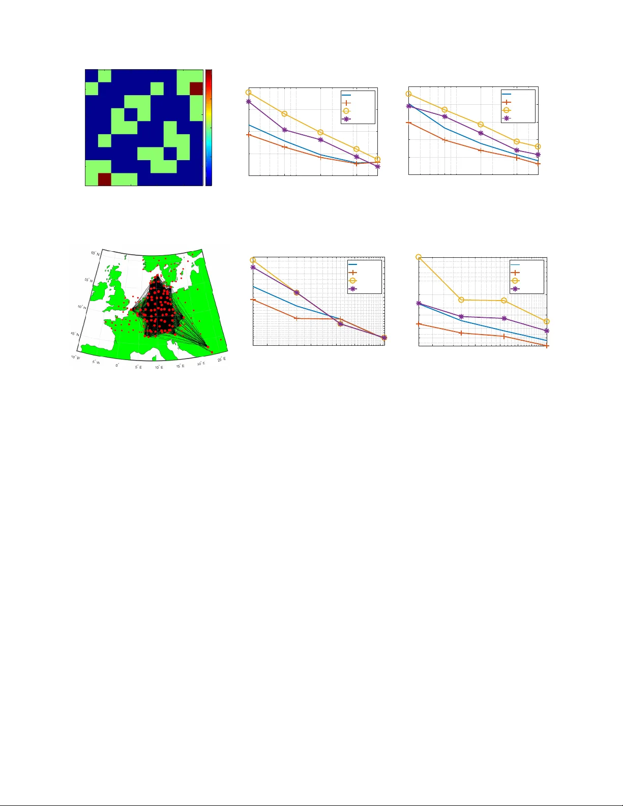
1 Gaussian Processes Ov er Graphs Arun V enkitaraman, Saikat Chatterjee, Peter H ¨ andel Department of Information Science and Engineering School of Electrical Engineering and Computer Science KTH Royal Institute of T echnology , SE-100 44 Stockholm, Sweden arun v@kth.se, sach@kth.se, ph@kth.se Abstract —W e propose Gaussian processes for signals over graphs (GPG) using the apriori knowledge that the target vectors lie over a graph. W e incorporate this inf ormation using a graph- Laplacian based regularization which enfor ces the target vectors to hav e a specific profile in terms of graph Fourier transform coeffcients, for example lowpass or bandpass graph signals. W e discuss how the regularization affects the mean and the variance in the prediction output. In particular , we prov e that the predictiv e variance of the GPG is strictly smaller than the con ventional Gaussian process (GP) for any non-trivial graph. W e validate our concepts by application to various real-world graph signals. Our experiments show that the performance of the GPG is superior to GP f or small training data sizes and under noisy training. Index T erms —Gaussian processes, Bayesian, graph signal pro- cessing, Linear model, kernel r egression, . I . I N T RO D U C T I O N Gaussian processes are a natural extension of the ubiquitous kernel regression to the Bayesian setting where the re gression parameters are modelled as random variables with a Gaussian prior distribution [1]. Giv en the training observations, Gaus- sian processes generate posterior probabilities of the target or output for new inputs or observations, as a function of the training data and the input kernel function [2]. Gaussian process models and its v ariants hav e been applied in a number of div erse fields such as model predicti ve control and system analysis [3]–[7], latent variable models [8]–[11], multi-task learning [10], [12], [13], image analysis and synthesis [14]– [17], speech processing [18]–[20], and magnetic resonance imaging (MRI) [21], [22]. Gaussian processes ha ve also been extended to a non-stationary regression setting [23]–[25] and for regression ov er complex-v alued data [26]. Recently , Gaus- sian processes were shown to be useful in training and analysis of deep neural networks, and that a Gaussian process can be viewed as a neural network with a single infinite-dimensional layer of hidden units [27], [28]. The prediction performance of the Gaussian process depends on the av ailability of training data, progressively improving as the training data size is increased. In many applications, howe v er , we are required to make predictions using a limited number of observations which may be further corrupted with observation noise. For such cases, providing additional structure helps improve the prediction performance of the GP significantly . In this article, we adv ocate the use of graph signal processing for improving prediction performance in the lack of sufficient and reliable training data. W e propose Gaussian processes by incorporating the apriori knowledge that the vector -valued tar get or output vectors lie ov er an underlying graph. This forms a natural Bayesian extension of the kernel regression for graph signals proposed recently in [29]. In particular , the target vectors are enforced to follo w a pre-specified profile in terms of the graph Fourier coefficients, such being lo wpass, bandpass, or high-pass. W e show that this in turn translates to a specific structure on the prior distribution of the target v ectors. W e deriv e the predictive distribution for a general input giv en the training observations, and prove that graph signal structure leads to decrease in variance of the predicti ve distribution. Our hypothesis is that incorporating the graph structure would boost the prediction performance. W e validate our hypothesis on v arious real-world datasets such as temperature measurements, flo w-cytometry data, functional MRI data, and tracer diffusion experiment for air pollution studies. Though we consider GPG mainly for undirected graphs characterized by the graph-Laplacian in our analysis, we also discuss ho w our approach may be e xtended to handle directed graphs using an appropriate regularization. I I . P R E L I M I N A RI E S O N G R A P H S I G NA L P R O C E S S I N G Graph signal processing or signal processing over graphs deals with extension of sev eral traditional signal processing methods while incorporating the graph structural information [30], [31]. This includes signal analysis concepts such as Fourier transforms [32], filtering [30], [33], wa velets [34], [35], filterbanks [36], [37], multiresolution analysis [38]– [40], denoising [41], [42], and dictionary learning [43], [44], and stationary signal analysis [45], [46]. Spectral clustering and principal component analysis approaches based on graph signal filtering hav e also been proposed recently [47], [48]. Sev eral approaches have been proposed for learning the graph directly from data [49], [50]. Recently , kernel regression based approaches hav e also been dev eloped for graph signals [29], [51], [52]. W e no w briefly re view the relev ant concepts from graph signal processing which will be used in our analysis and de velopment. This re vie w has been included to keep our article self-contained. A. Graph Laplacian and gr aph F ourier spectrum Consider an undirected graph with M nodes and adjacency matrix A . The ( i, j ) th entry of A denotes the strength of the 2 edge between the i th and j th nodes, A ( i, j ) = 0 denoting absence of edge. Since the graph is undirected, we hav e symmetric edge-weights or A = A > . The graph-Laplacian matrix L is defined as L = D − A , where D is the diagonal degree matrix with i th diagonal element giv en by the sum of the elements in the i th ro w of A [53]. L is symmetric for an undirected graph and by construction has nonnegati ve eigen v alues with the smallest eigen v alue being equal to zero. A graph signal y = [ y (1) y (2) · · · y ( M )] > ∈ R M is an M - dimensional vector such that y ( i ) denotes the value of the signal at the i th node, where > denotes transpose operation. The smoothness of y is measured using l ( y ) = y > Ly y > y = 1 y > y X A ( i,j ) 6 =0 A ( i, j )( y ( i ) − y ( j )) 2 . The quantity l ( y ) is small when y takes the similar v alue across all connected nodes, in agreement with what one intuitiv ely expects of a smooth signal. Similarly , y is a high-frequency or non-smooth signal if it has dissimilar v alues across connected nodes, or equi v alently a large value of l ( y ) . The eigen vectors of the graph-Laplacian are used to define the notion of frequency of graph signals. Let { λ i } M i =1 and { v i } M i =1 ∈ R M denote the eigen values and eigen vectors of L , respectiv ely . Then, the eigen value decomposition of L is L = VJ L V > , (1) where J L is the diagonal eigen v alue matrix of L , such that V = [ v 1 v 2 · · · v M ] and J L = diag ( λ 1 , λ 2 , · · · , λ M ) , It is standard practice to order the eigen vectors v i of the graph-Laplacian according to their smoothness in terms of l ( v i ) . The eigenv ectors v i are referred to as the graph Fourier transform (GFT) basis vectors since they generalize the notion of the discrete Fourier transform [31]. Let λ i denote the i th eigen v alue of L ordered as 0 = λ 1 ≤ λ 2 · · · ≤ λ M . Then, we observe that l ( v i ) = λ i . In other words, the eigen vectors corresponding to smaller λ i vary smoothly o ver the graph and those with large λ i exhibit more variation across the graph. This in turn giv es an intuitiv e frequency ordering of the GFT basis vectors. The GFT coefficients of a graph signal x are defined as the inner product of the signal with the GFT basis vectors V , that is, the GFT coefficient v ector ˆ x is defined as: ˆ x = V > x . The in v erse GFT is then gi ven by x = V ˆ x . A graph signal may then be lo w-pass or smooth, high-pass, band-pass, or band-stop according to the distrib ution of its GFT coefficients in ˆ x . B. Generative model for gr aph signals W e now deri ve the expressions for the graph signal of a particular GFT profile closest to any giv en signal, which shall be used in our analysis later . For any signal y , a graph signal with a specified graph frequency profile y g closest to y can be obtained by solving the following generativ e model y g = arg min z k y − z k 2 2 + α k J p ˆ z k 2 2 , α ≥ 0 where ˆ z = V > z is the GFT of z and J p = diag( J (1) , J (2) , · · · , J ( M )) is the diagonal matrix whose values penalize or promote specific GFT coefficients. For example, if z is to hav e energy predominantly in GFT v ectors with indices { i, j, k , l } , we set the corresponding diagonal entries of J p to zero and assign large v alues to the remaining diagonal entries. From the properties of the GFT , we hav e that k J p ˆ z k 2 2 = ˆ z > J 2 p ˆ z = z > VJ 2 p V > z = z > Gz , where G = VJ 2 p V > . Then, the generative model is equiv a- lently expressible as: y g = arg min z k y − z k 2 2 + α z > Gz , α ≥ 0 . (2) Since all the eigen v alues of G are nonnegati ve, G is positiv e semidefinite giving the unique closed-form solution for y g as y g = ( I M + α G ) − 1 y . (3) W e note that most graph signals encountered in practice are usually smooth over the associated graph. One of the simplest cases of generating a smooth graph signal is to penalize the frequencies linearly by setting J ( i ) = √ λ i . This in turn corresponds to G = VJ L T > = L and the smooth graph signal then becomes y g = ( I M + α L ) − 1 y . I I I . G AU S S I A N P R O C E S S O V E R G R A P H W e first dev elop Bayesian linear regression ov er graph and then proceed to de velop a Gaussian process o ver graph. A. Bayesian linear r e gr ession over graph W e now propose linear re gression ov er graphs. Let { x n } N n =1 denote the set of N input observ ations, n = 1 , · · · , N and t n ∈ R M denote the corresponding vector target v alues. W e model the tar get as the output of a linear regression such that t n = y ( x n , W ) + e n , (4) where e n denotes the additiv e noise vector follo wing a zero mean isotropic Gaussian distrib ution, that is, p ( e n ) = N ( e n | 0 , β − 1 I M ) . (5) Here I M denotes the identity matrix of dimension M and β is the precision parameter for the noise. The signal y is y ( x n , W ) = W > φ φ φ ( x n ) , y n , where φ φ φ ( x ) ∈ R K is a function of x , W ∈ R K × M denotes the regression coefficient matrix. W e further consider an isotropic Gaussian prior with precision γ for the entries of W . Let us use the notation ˜ w , vec ( W ) where v ec ( W ) denotes the vectorization of W obtained by concatenating the columns of W into a single vector . Then, we have that p ( ˜ w ) = N ( ˜ w | 0 , γ − 1 I K M ) . (6) Our principal assumption is that the predicted tar get vector or regression output y n has a graph Fourier spectrum as characterized by the diagonal spectrum matrix J p . Howe ver , y n is not necessarily satisfy this requirement for an arbitrary choice of W , since φ φ φ ( · ) is also fixed apriori and has not been 3 assumed to be graph-specific. It becomes clear then that the prior on ˜ w should be chosen in a way that it promotes y n to ha ve the required graph Fourier spectrum. W e next discuss our strategy for formulating such a prior distribution. Giv en the regression output y n generated using a fixed W dra wn from (6), the graph signal y g ,n closest to y n is obtained by using the generative model (2) with the following result y g ,n = ( I M + α G ) − 1 y n = ( I M + α G ) − 1 W > φ φ φ ( x n ) = W > g φ φ φ ( x n ) , where W g , W ( I M + α G ) − 1 . Let B = ( I M + α G ) − 1 , then we have that W g = WB . (7) Thus, we note that regression of φ φ φ ( x ) with re gression coef fi- cient matrix W g produces graph signals possessing the desired graph Fourier profile. In the case of G = L , this is the same as regression output being smooth ov er the graph. On vectorizing both sides of (7) and using properties of the Kronecker product [54], we get that ˜ w g , vec ( W g ) = vec ( WB ) = ( B ⊗ I K ) ˜ w , where ⊗ denotes the Kronecker product operation. Note that B is symmetric as L and hence, G is symmetric. Since p ( ˜ w ) = N ( vec ( ˜ w ) | 0 , γ − 1 I K M ) , we get that ˜ w g is distributed according to p ( ˜ w g ) = N ( ˜ w g | 0 , γ − 1 ( B 2 ⊗ I K )) . (8) This in turn implies that choosing a prior for the regression coefficients of the form (8) yields graph signals with specified graph Fourier spectrum over the graph with the Laplacian matrix L . W e then pose the regression problem (9) in the following form t n = y g ( x n , W g ) + e 0 n , W e assume that e 0 n follows the same distrib ution of e n in (9). Then, the conditional distrib ution of t n is giv en by p ( t n | X , W g , β ) = N ( t n | W > g φ φ φ ( x n ) , β − 1 I M ) . (9) W e define the matrices Φ , Y g , and T as follows: Φ = [ φ φ φ ( x 1 ) φ φ φ ( x 2 ) · · · φ φ φ ( x N )] > , Y g = [ y g , 1 y g , 2 · · · y g ,N ] T , T = [ t 1 t 2 · · · t N ] T . On accumulating all the observations we hav e ˜ t = ˜ y g + ˜ e (10) where ˜ t , v ec( T ) , ˜ y g , vec( Y g ) and ˜ e is the noise term. Dropping the dependency of the distrib ution on X , W g , β for brevity , we have that p ( ˜ t ) = N ( ˜ t | ˜ y , β − 1 I M N ) . (11) Since Y g = ΦW g , we have that ˜ y = vec ( ΦW g ) = vec ( ΦWB ) = ( B > ⊗ Φ ) vec ( W ) = ( B ⊗ Φ ) ˜ w . The prior distribution of ˜ y is then a multiv ariate Gaussian distribution with mean and co variance gi ven by E { ˜ y } = ( B ⊗ Φ ) E { ˜ w } = 0 , (12) E { ˜ y ˜ y > } = ( B ⊗ Φ ) E { ˜ w ˜ w > } ( B ⊗ Φ ) > = γ − 1 ( B ⊗ Φ )( B > ⊗ Φ > ) = γ − 1 ( B 2 ⊗ ΦΦ > ) . W e refer to this model as Bayesian linear r e gr ession over graph . B. Gaussian pr ocess over gr aph W e next dev elop Gaussian process over graphs (GPG). W e first note the e xistence of ΦΦ > in (12) and that the input x n enters the equation only in the form of inner products of φ φ φ ( · ) . The inner product φ φ φ ( x n ) > φ φ φ ( x m ) is a measure of similarity between the m th and n th inputs. Keeping this in mind, one may generalize the inner-product φ φ φ ( x m ) > φ φ φ ( x n ) to any v alid kernel function [2] k ( x m , x n ) of the inputs x m and x n . The kernel matrix is denoted by K = γ − 1 ΦΦ > , and its ( m, n ) th entry is k ( x m , x n ) . Following (10), (11), and (12) we find that ˜ t is Gaussian distributed with zero mean and follo wing cov ariance C g ,N = ( B 2 ⊗ K ) + β − 1 I M N , (13) where we use the first subscript g to denote the graph, and the second subscript N to sho w explicit dependency on N observations. W ith ( N + 1) samples, we have that C g ,N +1 =  C g ,N D D > F  , where D = B 2 ⊗ k , k = [ k ( x N +1 , x 1 ) , k ( x N +1 , x 2 ) , · · · , k ( x N +1 , x N )] > , and F = k ( x N +1 , x N +1 ) B 2 + β − 1 I M . Then, using properties of conditional probability for jointly Gaussian vectors [2], we have the predicti ve distribution of GPG as follows p ( t N +1 | t 1 , · · · , t N ) = N ( t N +1 | µ µ µ N +1 , Σ N +1 ) , (14) where µ µ µ N +1 = D > C − 1 g ,N ˜ t and Σ N +1 = F − D > C − 1 g ,N D . W e note that in the case of completely disconnected graph, which corresponds to the conv entional Gaussian process (GP), the graph adjacency matrix is equal to the identity matrix and correspondingly , L = 0 . Then, the cov ariance of the joint distribution of ˜ t is given by C c,N = ( I M ⊗ K ) + β − 1 I M N , where the subscript c denotes it being the con ventional Gaus- sian process. Correspondingly , the predicti ve distribution of t N +1 is giv en by p ( t N +1 | t 1 , · · · , t N ) = N ( t N +1 | µ µ µ c,N +1 , Σ c,N +1 ) , where µ µ µ c,N +1 = D > c C − 1 c,N ˜ t , Σ c,N +1 = F c − D > c C − 1 c,N D c , 4 D c = I M ⊗ k , F c = ( k ( x N +1 , x N +1 ) + β − 1 ) I M . W e note that since Bayesian linear regression on graphs dev eloped in Section A is a special case of the Gaussian process on graphs with kernels, we shall refer to the former as Gaussian pr ocess-Linear (GPG-L) and the latter as Gaussian pr ocess-K ernel (GPG-K) . Correspondingly , we refer to the con ventional versions as GP-L, and GP-K, respecti vely . W e ne xt show that use of graph information reduces the variance of the predicti ve distribution. This implies that the GPG models the observed training samples better than con- ventional GP . Theorem 1 (Reduction in v ariance) . Gr aph structur e reduces the variance of the marginal distribution p ( ˜ t ) , that is, GPG r esults in smaller variance of p ( ˜ t ) than GP: tr ( C c,N ) > tr ( C g ,N ) . Pr oof. In order to prove the result, we need to sho w that the trace of ∆ C N := C c,N − C g ,N is nonnegativ e. Using the properties of trace operation, we have that tr(∆ C N ) = tr( C c,N − C g ,N ) = tr(( I M − B 2 ) ⊗ K ) = tr( I M − B 2 ) tr ( K ) Since K is positiv e semidefinite by construction as a ker- nel matrix, we have that tr(∆ C N ) ≥ 0 if and only if tr( I M − B 2 ) ≥ 0 . Let { θ i } N i =1 and { u i } N i =1 ∈ R N denote the eigen values and eigen v ectors of K , respecti v ely . Then, the eigen v alue decomposition of G and K are gi ven by G = VJ G V > , K = UJ K U > , where J K and J G denote the diagonal eigen v alue matrix of K and G , respecti vely , such that V = [ v 1 v 2 · · · v M ] J G = diag ( J 2 (1) , J 2 (2) , · · · , J 2 ( M )) , U = [ u 1 u 2 · · · u N ] and J K = diag ( θ 1 , θ 2 , · · · , θ N ) . Since J G = J 2 p = diag( J 2 (1) , J 2 (2) , · · · J 2 ( M )) , we have tr( I M − B 2 ) > 0 , tr( I M − V ( I + α J G ) − 2 V > ) ≥ 0 , tr( I M − ( I M + α J G ) − 2 ) ≥ 0 , M X i =1  1 − 1 (1 + α J ( i )) 2  ≥ 0 . Let s denote the graph eigen v alue index corresonding to the denote the smallest non-zero diagonal v alue in J p , the value gi ven by J ( s ) . Then, we have that 1 (1 + α J 2 ( i )) ≤ 1 (1 + α J 2 ( s )) ∀ J 2 ( i ) 6 = 0 . Then, a sufficient condition to ensure tr( I M − B 2 ) ≥ 0 is to impose that (1 + α J 2 ( s )) − 2 ≤ 1 , (1 + α J 2 ( s )) ≥ 1 , αJ 2 ( s ) ≥ 0 . A graph with atleast one connected subgraph has atleast one eigen v alue of L strictly greater than 0 [53]. Thus, barring the completely disconnected graph and the pathological case of J p = 0 (or G = 0 ), any graph with connections across nodes results in αJ 2 ( s ) > 0 or in other words that the variance strictly reduces in comparison with the conv entional regression, that is, tr(∆ C N ) > 0 . In other words, introducing non-zero connections among the nodes ensures that the marginal variance is strictly lesser than that obtained for the conv entional regression case. W e also note that in order for the reduction in variance to be significant, λ s must be large, which in turn implies that the connected communities within the graph must hav e strong algebraic connectivity [53]. In the case of regression output being smooth graph signals in the sense of G = L , we ha ve that J 2 ( i ) = λ i and s = K for a graph with K -connected components or disjoint subgraphs. This is because the number of zero eigen v alues of L is equal to the nunber of connected components in the graph [53], [55]. An immediate consequence of the Theorem is the following important Corrollary which informs us that the v ariance of the predicted tar get reduces when the graph signal structure is employed: Corollary 1.1 (Reduction in predicti ve v ariance) . GPG-K with a non-trivial graph has strictly smaller pr edictive variance than GPG-K, that is, tr ( Σ c,N +1 ) > tr ( Σ g ,N +1 ) . Pr oof. W e are required to prov e that tr ( Σ c,N +1 − Σ g ,N +1 ) > 0 , or equi valently that ∆ Σ Σ Σ := Σ c,N +1 − Σ g ,N +1 is a positiv e semidefinite matrix. W e notice that ∆ C N +1 is giv en by ∆ C N +1 =  ∆ C N D c − D D > c − D > F c − F  . W e observe that ∆ Σ Σ Σ N +1 is then the Schur complement of F c − F in ∆ C N +1 . Since the Schur complement of a positiv e- definite matrix is also positiv e-definite [56], and we have already proved that ∆ C N +1 is positive-definite from Theorem 1, it follows that tr ( Σ c,N +1 − Σ g ,N +1 ) > 0 , or tr ( Σ g ,N +1 ) < tr ( Σ c,N +1 ) . By the preceding analysis, we also observe that the v ariance of the joint distribution C g ,N +1 , and hence, that of Σ Σ Σ g ,N +1 is in versely related to the graph regularization parameter α . This is because a large α implies a small v alue of 1 1 + α J 2 ( i ) for all i , and therefore, a small v alue of tr ( C g ,N +1 ) . 5 C. On the mean vector of pr edictive distrib ution W e no w sho w that the mean of predicti ve distribution is a graph signal with a graph Fourier spectrum which adheres to the condition imposed by J p . W e demonstrate this by computing the graph F ourier spectrum of the predicti ve mean. Using the eigendecompostions of G and K , we hav e that µ µ µ N +1 = D > C − 1 g ,N ˜ t = D > ( B 2 ⊗ K + β − 1 I M N ) − 1 ˜ t = D > ( V ( I + α J G ) − 2 V > ⊗ UJ K U > + β − 1 I M N ) − 1 ˜ t = D > ( V ⊗ U ) J ( V > ⊗ U > ) ˜ t = D > ( ZJZ > ) ˜ t = D > M N X i =1 η i ρ i z i where J = (( I + α J G ) − 2 ⊗ J K + β − 1 I M N ) − 1 , η i is the i th diagonal element of J , Z = V ⊗ U , z i denotes the i th column vector of Z , and ρ i = z > i ˜ t . Since the η i is a function of some i 1 th eigen v alue of L and i 2 th eigen v alue of K , we shall alternatively use the notation η i 1 ,i 2 to be more specific in the following analysis. Similarly , ρ i expressed as ρ i 1 ,i 2 and the eigen vectors z i = v i 1 ⊗ u i 2 . The component of the prediction mean along the graph eigenv ector v k (or the k th graph frequenc y) is then gi ven by µ µ µ > N +1 v k = M N X i =1 η i ρ i z > i Dv k = M N X i =1 η i ρ i z > i ( B 2 ⊗ k ) v k = M N X i =1 η i ρ i ( v > i 1 ⊗ u > i 2 )( B ⊗ k ) v k = M N X i =1 η i ρ i ( v > i 1 B ⊗ u > i 2 k ) v k = M N X i =1 η i ρ i ( v > i 1 V ( I + α J G ) − 2 V > ⊗ u > i 2 k ) v k = M X i 1=1 N X i 2=1 η i 1 ,i 2 ρ i 1 ,i 2 ((1 + α J 2 ( i 1)) − 2 v > i 1 ⊗ u > i 2 k ) v k = M X i 1=1 N X i 2=1 η i 1 ,i 2 ρ i 1 ,i 2 u > i 2 k (1 + α J 2 ( i 1)) − 2 ( v > i 1 ) v k = N X i 2=1 η k,i 2 ρ k,i 2 u > i 2 k (1 + α J 2 ( k )) − 2 v > k v k = 1 (1 + α J 2 ( k )) 2 M N X i =1 η k,i 2 ρ k,i 2 u > i 2 k = 1 (1 + α J 2 ( k )) 2 N X l =1 ρ k,i 2 u > i 2 k β θ i 2 (1 + α J 2 ( k )) 2 β θ i 2 + (1 + αJ ( k )) 2 = N X i 2=1 ρ k,i 2 u > i 2 k β θ i 2 β θ i 2 + (1 + αJ 2 ( k )) 2 . W e observe that a nonzero α reduces or shrinks the con- tribution from the graph-frequencies corresponding to larger J 2 ( k ) , in comparison with the con v entional mean obtained by setting α = 0 . In the case of smooth graph signals, we hav e J 2 ( k ) = λ k implying that the prediction mean has lo wer contributions from higher graph-frequencies, which in turn shows that GPG performs a noise-smoothening by making use of the graph topology . Howe ver , this does not imply that the value of α may be set to be arbitrarily lar ge. A large α will in turn force the resulting target predictions to lie close to the smoother eigen v ectors of L , which is not desirable since it reduces the learning ability of the GP . W e note that since GPG-L is a special case of the GPG-K, Theorem 1 and the analysis following it apply directly also to GPG-L. D. Extension for dir ected graphs In our analysis, we ha ve assumed the underlying graph for the target vectors to be undirected and hence, characterized by the symmetric positi ve semidefinite graph-Laplacian matrix L . W e now discuss ho w GPG may be deri ved for the case of directed graphs, that is, when the adjacency matrix of the graph is assymetric. In the case of directed graphs, the following metric is popular for quantifying the smoothness of the graph signals: MS g ( y ) = k y − Ay k 2 2 , where y and A denote the graph signal and adjacenc y matrix, respectiv ely , the adjacency matrix assumed to be normalized to have maximum eigen value modulus equal to unity [30]. A signal y is smooth over a directed graph if it has a small MS g value. This is because MS g measures the difference between the signal and its one-step diffused or ’graph-shifted’ version, thereby measuring the difference between the signal v alue at each node and its neighbours, weighted by the strength of the edge between the nodes. In the case of directed graphs, we may adopt the same approach as that of the undirected graph case with one important distinction: instead of solving (2), we now solv e the follo wing problem for each observ ation: y 0 n = arg min z k y n − z k 2 2 + α MS g ( z ) , = arg min z k y n − z k 2 2 + α z > ( I − A ) > ( I − A ) z , Then, we have that y 0 n =  I M + α ( I − A ) > ( I − A )  − 1 y n . Using a similar analysis as with the undirected graph case, we arriv e at the follo wing Gaussian process model: ˜ t = ˜ y + ˜ e , where ˜ y is distrib uted according to the prior: p ( ˜ y ) = N ( ˜ y | 0 , ( B 2 d ⊗ K )) , where B d =  I M + α ( I − A ) > ( I − A )  − 1 . By following similar analysis as with the undirected graphs, it is possible to show that the variance of the predictive distribution reduces using GPG and that the predictiv e mean is smooth over the graph. In the interest of space and to av oid repetition, we do not include the analysis for directed graphs here. 6 I V . E X P E R I M E N T S W e consider application of GPG to v arious real-world signal examples. For the examples, we consider undirected graphs. Our interest is to compute the predicti ve distrib ution (14) gi ven the noisy targets T and the corresponding inputs X . Our assumption is that a target vector is smooth over an underlying graph. W e use the graph-regularization with G = L . T o ev aluate the prediction performance, we use the normalized- mean-square-error (NMSE) defined as follows: NMSE = 10 log 10  E k Y − T 0 k 2 F E k T 0 k 2 F  , where Y denotes the mean of the predicti ve distrib ution and T 0 the true v alue of tar get matrix, that means T 0 does not con- tain any noise. The noisy target matrix T is generated obtained by adding white Gaussian noise with precision parameter β to T 0 . In the case of real-world examples, we compare the performance of the follo wing cases: 1) GP with linear regression (GP-L): k m,n = γ − 1 φ φ φ ( x m ) > φ φ φ ( x n ) , where φ φ φ ( x ) = x and α = 0 , 2) GPG with linear re gression (GPG-L): k m,n = γ − 1 φ φ φ ( x m ) > φ φ φ ( x n ) and α > 0 , where φ φ φ ( x ) = x , 3) GP with kernel regression (GP-K): Us- ing radial basis function (RBF) kernel k m,n = γ − 1 exp  − k x m − x n k 2 2 σ 2  and α = 0 , and 4) GPG with kernel regression over graphs (GPG-K): Using RBF kernel k m,n = γ − 1 exp  − k x m − x n k 2 2 σ 2  and α > 0 . W e use five-fold cross-validation to obtain the values of regularization parameters α and γ . W e set the kernel parameter σ 2 = X m,n k x m − x n k 2 2 . W e perform experiments under various signal-to-noise ratio (SNR) levels, and choose the precision parameter β accordingly . A. Prediction for fMRI in cer ebellum graph W e first consider the functional magnetic resonance imaging (fMRI) data obtained for the cerebellum region of brain [57] 1 . The original graph consists of 4465 nodes corresponding to different voxels of the cerebellum region. The voxels are mapped anatomically following the atlas template [58], [59]. W e refer to [57] for details of graph construction and associated signal extraction. W e consider a subset of the first 100 vertices in our analysis. Our goal is to use the first ten vertices as input x ∈ R 10 to make predictions for remaining 90 vertices, which forms the output t ∈ R 90 . Thus, the target signals lie ov er a graph of dimension M = 90 . The corresponding adjacency matrix is sho wn in Figure 1(a). W e hav e a total of 295 graph signals corresponding to dif ferent measurements from a single subject. W e use a portion of the signals for training and the remaining for testing. W e construct 1 The data is av ailable publicly at https://openfmri.org/dataset/ds000102. noisy training targets by adding white Gaussian noise at SNR- lev els of 10 dB and 0 dB. The NMSE of the prediction mean for testing data, av eraged over 100 different random choices of training and testing sets is shown in 1(b) and (c); this is Monte Carlo simulation to check rob ustness. W e observe that for both linear and kernel regression cases, GPG outperforms GP by a significant margin, particularly at small training data sizes as expected. The trend is also similar when larger subsets of nodes from the full set are considered. The results are not reported here for bre vity and to a void repetition. B. Prediction for temperatur e data W e next apply GPG on temperature measurements from the 45 most populated cities in Sweden for a period of three months from October to December 2017. The data is available publicly from the Swedish Meteorological and Hydrological Institute [60]. Our goal is to perform one-day temperature prediction: giv en the temperature data for a particular day x n , we predict the temperature for the next day t n . W e have 90 input-target data pairs in total, of which one half is used for training and the rest for testing. W e consider the geodesic graph in our analysis with the ( i, j ) th entry of the graph adjacency matrix A is gi ven by A ( i, j ) = exp − d 2 ij P i,j d 2 ij ! , where d ij denotes the geodesic distance between the i th and j th cities. In order to remov e self loops, the diagonal of A is set to zero. W e generate noisy training data by adding zero-mean white Gaussian noise at SNR of 5 dB and 0 dB to the true temperature measurements. In Figure 2, we sho w the NMSE obtained for testing data by a veraging ov er 100 different random partitioning of the total dataset into training and testing datasets. W e observe that GPG outperforms GP for both linear and kernel regression cases. C. Prediction for flow-cytometry data W e now consider the application of GPG to flo w-cytometry data considered by Sachs et al. [61] which consists of response or signalling level of 11 proteins in dif ferent experiment cells. Since the protein signal v alues hav e a large dynamic range and are all positive values, we perform experiments on signals obtained by taking a logarithm with the base of 10 for reducing the dynamic range. W e use the first 1000 measurements in our analysis. W e use the symmetricized version of the directed unweighted acyclic graph proposed by Sachs et al. [61]. Among the 11 proteins, we choose proteins 10 and 11 arbitrarily as input to make predictions for the remaining 9 proteins which forms the target vector y n ∈ R 7 lying on a graph of M = 7 nodes. W e perform the experiment 100 times in Monte Carlo simulation, where we random divide the total dataset into training and testing datasets. The average NMSE for testing datasets is shown in Figure 3 at SNR lev els of 5 dB and 0 dB. W e once again observe the same trend that GPG outperforms GP for both linear and kernel cases at low sample sizes corrupted with noise. 7 20 40 60 80 20 40 60 80 0 0.2 0.4 0.6 0.8 1 (a) 4 14 24 34 44 Training sample size N -25 -20 -15 -10 -5 NMSE GP-L GPG-L GP-K GPG-K (b) 4 14 24 34 44 Training sample size N -20 -15 -10 -5 0 NMSE GP-L GPG-L GP-K GPG-K (c) Fig. 1. Results for the cerebellum data (a) Adjacency matrix, (b) NMSE for testing data as a function of training data size at SNR= 10 dB, and (c) at SNR= 0 dB. 5 10 15 20 25 5 10 15 20 25 0 0.01 0.02 0.03 0.04 0.05 (a) 4 14 24 34 44 Training sample size N -16 -14 -12 -10 -8 NMSE GP-L GPG-L GP-K GPG-K (b) 4 14 24 34 44 Training sample size N -14 -12 -10 -8 -6 -4 NMSE GP-L GPG-L GP-K GPG-K (c) Fig. 2. Results for the temperature data (a) Adjacency matrix, (b) NMSE for testing data as a function of training data size at SNR= 5 dB, and (c) at SNR= 0 dB. Number 1 2 3 4 5 6 7 8 9 10 11 Name praf pmek plcg PIP2 PIP3 p44/42 pjnk pakts473 PKA PKC P38 T ABLE I N A M E S O F D IFF E R EN T P R OT EI N S T H A T R EP R E S EN T T H E N O DE S O F T H E G R AP H C O N S ID E R E D IN S E CT I O N I V - D. D. Prediction for atmospheric tracer diffusion data Our next experiment is on the atmospheric tracer dif fusion measurements obtained from the European T racer Experiment (ETEX) which tracked the concentration of perfluorocarbon tracers released into the atmosphere starting from a fix ed lo- cation (Rennes, France) [62]. The observations were collected from two experiments o ver a span of 72 hours at 168 ground stations over Europe, gi ving two sets of 30 measurements, in total 60 measurements. Our goal is to predict the tracer concentrations on one half (84) of the total ground stations, using the concentrations at the remaining locations. The target signal t n is then a graph signal over a graph of M = 84 nodes where n denotes the measurement index. The corresponding input vector x n is also of length 84. W e illustrate the ground station locations in a schematic in Figure 4 (a). The output nodes which correspond to the the tar get are shown in red markers with corresponding edges, whereas the rest of the markers denote the input. W e simulate noisy training by adding white Gaussian noise at different SNR levels to the training data. W e consider a geodesic distance based graph. The graph is constructed in the same manner like the graph used in the temperature data e xperiment previously . W e randomly di vide the total dataset of 60 samples equally into training and test datasets. W e compute the NMSE for the dif ferent approaches by av eraging over 100 different randomly drawn training subsets of size N from the full training set of size N ts = 30 . W e plot the NMSE as a function of N in Figures 4(b)-(c) at SNR lev els of 5 dB and 0 dB. W e observ e that graph structure enhances the prediction performance signficantly under noisy and low sample size conditions. V . R E P R O D U C I B L E R E S E A R C H In the spirit of reproducible research, all the codes relev ant to the experiments in this article are made a vailable at https://www .researchgate.net/profile/Arun V enkitaraman and https://www .kth.se/ise/research/reproducibleresearch- 1.433797. V I . C O N C L U S I O N S W e developed Gaussian processes for signals over graphs by employing a graph-Laplacian based regularization. The Gaussian process over graphs was shown to be a consistent generalization of the conv entional Gaussian process, and that it pro v ably results in a reduction of uncertainty in the output prediction. This in turn implies that the Gaussian process over graph is a better model for tar get vectors lying o ver a graph in comparison to the con ventional Gaussian process. This observation is important in cases when the av ailable training 8 2 4 6 8 2 4 6 8 0 0.5 1 1.5 2 (a) 4 8 16 32 48 Training sample size N -12 -10 -8 -6 -4 NMSE GP-L GPG-L GP-K GPG-K (b) 4 8 16 32 48 Training sample size N -12 -10 -8 -6 -4 -2 NMSE GP-L GPG-L GP-K GPG-K (c) Fig. 3. Results for flow-cytometry data (a) Adjacency matrix, (b) NMSE for testing data as a function of training data size at SNR= 5 dB, and (c) at SNR= 0 dB. (a) 5 10 15 20 25 30 Training sample size N -7 -6 -5 -4 -3 -2 NMSE GP-L GPG-L GP-K GPG-K (b) 5 10 15 20 25 30 Training sample size N -5 -4 -3 -2 -1 -0.5 NMSE GP-L GPG-L GP-K GPG-K (c) Fig. 4. Results for ETEX data (a) Schematic showing the ground stations for the experiment, (b) NMSE for testing data as a function of training data size at SNR= 5 dB, and (c) at SNR= 0 dB. data is limited in both quantity and quality . Our expectation and motiv ation was that incorporating the graph structural information would help the Gaussian process make better predictions, particularly in absence suf ficient and reliable training data. The experimental results with the real-world graph signals illustrated that this is indeed the case. R E F E R E N C E S [1] C. E. Rasmussen and C. K. I. Williams, Gaussian Pr ocesses for Mac hine Learning (Adaptive Computation and Machine Learning) . The MIT Press, 2005. [2] C. M. Bishop, P attern Recognition and Machine Learning (Information Science and Statistics) . Secaucus, NJ, USA: Springer-V erlag New Y ork, Inc., 2006. [3] G. Cao, E. M. K. Lai, and F . Alam, “Gaussian process model predictive control of unknown non-linear systems, ” IET Control Theory Appl. , vol. 11, no. 5, pp. 703–713, 2017. [4] G. Chowdhary , H. A. Kingravi, J. P . How , and P . A. V ela, “Bayesian nonparametric adaptive control using Gaussian processes, ” IEEE T rans- actions on Neur al Networks and Learning Systems , v ol. 26, no. 3, pp. 537–550, March 2015. [5] M. Stepan ˇ ci ˇ c and J. Kocijan, “On-line identification with re gularised ev olving Gaussian process, ” IEEE Evolving and Adaptive Intelligent Systems (EAIS) , pp. 1–7, May 2017. [6] H. Soh and Y . Demiris, “Spatio-temporal learning with the online finite and infinite echo-state Gaussian processes, ” IEEE T rans. Neural Netw . Learn. Syst. , vol. 26, no. 3, pp. 522–536, March 2015. [7] G. Chowdhary , H. A. Kingravi, J. P . How , and P . A. V ela, “Bayesian nonparametric adaptiv e control using Gaussian processes, ” IEEE Tr ans. Neural Netw . Learn. Syst. , vol. 26, no. 3, pp. 537–550, March 2015. [8] G. Song, S. W ang, Q. Huang, and Q. T ian, “Multimodal similarity Gaussian process latent variable model, ” IEEE T rans. Image Pr ocess. , vol. 26, no. 9, pp. 4168–4181, Sept 2017. [9] N. Lawrence, “Probabilistic non-linear principal component analysis with Gaussian process latent variable models, ” J. Mach. Learn. Res. , vol. 6, pp. 1783–1816, 2005. [10] S. P . Chatzis and D. K osmopoulos, “ A latent manifold marko vian dynamics Gaussian process, ” IEEE T rans. Neural Netw . Learn. Syst. , vol. 26, no. 1, pp. 70–83, Jan 2015. [11] G. Chowdhary , H. A. Kingravi, J. P . How , and P . A. V ela, “Bayesian nonparametric adaptiv e control using gaussian processes, ” IEEE Tr ans. Neural Netw . Learn. Syst. , vol. 26, no. 3, pp. 537–550, March 2015. [12] K. Y u, V . Tresp, and A. Schw aighofer, “Learning Gaussian processes from multiple tasks, ” in Pr oceedings of the 22Nd International Confer ence on Machine Learning , ser. ICML ’05. New Y ork, NY , USA: A CM, 2005, pp. 1012–1019. [Online]. A vailable: http: //doi.acm.org/10.1145/1102351.1102479 [13] E. V . Bonilla, K. M. Chai, and C. Williams, “Multi-task Gaussian process prediction, ” in Advances in Neural Information Pr ocessing Systems 20 , J. C. Platt, D. Koller , Y . Singer, and S. T . Roweis, Eds. Curran Associates, Inc., 2008, pp. 153–160. [Online]. A vailable: http: //papers.nips.cc/paper/3189- multi- task- gaussian- process- prediction.pdf [14] H. W ang, X. Gao, K. Zhang, and J. Li, “Single image super-resolution using Gaussian process regression with dictionary-based sampling and student- t likelihood, ” IEEE T rans. Image Process. , vol. 26, no. 7, pp. 3556–3568, July 2017. [15] H. He and W . C. Siu, “Single image super -resolution using Gaussian process regression, ” in CVPR , June 2011, pp. 449–456. [16] Y . Kwon, K. I. Kim, J. T ompkin, J. H. Kim, and C. Theobalt, “Efficient learning of image super-resolution and compression artif act remov al with semi-local Gaussian processes, ” IEEE T rans. P attern Analysis Machine Intelligence , vol. 37, no. 9, pp. 1792–1805, Sept 2015. [17] R. L. de Queiroz and P . A. Chou, “Transform coding for point clouds using a Gaussian process model, ” IEEE Tr ans. Image Process. , vol. 26, no. 7, pp. 3507–3517, July 2017. [18] T . Koriyama, T . Nose, and T . Kobayashi, “Statistical parametric speech synthesis based on Gaussian process regression, ” IEEE J. Selected T opics iSignal Process. , vol. 8, no. 2, pp. 173–183, April 2014. [19] T . Koriyama, S. Oshio, and T . Kobayashi, “ A speaker adaptation 9 technique for Gaussian process regression based speech synthesis us- ing feature space transform, ” IEEE Intl. Conf. Acoust. Speech Signal Pr ocess. , pp. 5610–5614, March 2016. [20] D. Moungsri, T . Koriyama, and T . Kobayashi, “Duration prediction using multiple Gaussian process experts for gpr-based speech synthesis, ” IEEE Intl. Conf. Acoust. Speech Signal Process. , pp. 5495–5499, March 2017. [21] J. Sj ¨ olund, A. Eklund, E. ¨ Ozarslan, and H. Knutsson, “Gaussian process regression can turn non-uniform and undersampled dif fusion mri data into diffusion spectrum imaging, ” IEEE Intl. Symp. Biomedical Imaging (ISBI) , pp. 778–782, April 2017. [22] H. Bertrand, M. Perrot, R. Ardon, and I. Bloch, “Classification of mri data using deep learning and Gaussian process-based model selection, ” IEEE Intl. Symp. Biomedical Imaging (ISBI) , pp. 745–748, April 2017. [23] L. Mu ˜ noz-Gonz ´ alez, M. L ´ azaro-Gredilla, and A. R. Figueiras-V idal, “Laplace approximation for divisiv e Gaussian processes for nonstation- ary regression, ” IEEE T rans. P attern Analysis Machine Intelligence , vol. 38, no. 3, pp. 618–624, March 2016. [24] ——, “Divisi ve Gaussian processes for nonstationary regression, ” IEEE T rans. Neural Netw . Learn. Syst. , vol. 25, no. 11, pp. 1991–2003, Nov 2014. [25] S. P . Chatzis and Y . Demiris, “Nonparametric mixtures of Gaussian processes with power-la w behavior , ” IEEE Tr ans. Neural Netw . Learn. Syst. , vol. 23, no. 12, pp. 1862–1871, Dec 2012. [26] R. Boloix-T ortosa, E. Arias-de-Reyna, F . J. Payan-Somet, and J. J. Murillo-Fuentes, “Complex-v alued gaussian processes for regression: A widely non-linear approach, ” CoRR , vol. abs/1511.05710, 2015. [Online]. A vailable: http://arxi v .org/abs/1511.05710 [27] A. C. Damianou and N. D. Lawrence, “Deep Gaussian Processes, ” ArXiv e-prints , Nov . 2012. [28] K. Cutajar, E. V . Bonilla, P . Michiardi, and M. Filippone, “Random Feature Expansions for Deep Gaussian Processes, ” ArXiv e-prints , Oct. 2016. [29] A. V enkitaraman, S. Chatterjee, and P . H ¨ andel, “Kernel Regression for Signals over Graphs, ” ArXiv e-prints , Jun. 2017. [30] A. Sandryhaila and J. M. F . Moura, “Discrete signal processing on graphs, ” IEEE Tr ans. Signal Process. , v ol. 61, no. 7, pp. 1644–1656, 2013. [31] D. I. Shuman, S. Narang, P . Frossard, A. Ortega, and P . V andergheynst, “The emerging field of signal processing on graphs: Extending high- dimensional data analysis to networks and other irregular domains, ” IEEE Signal Process. Mag. , vol. 30, no. 3, pp. 83–98, 2013. [32] D. I. Shuman, B. Ricaud, and P . V andergheynst, “ A windowed graph Fourier transform, ” IEEE Statist. Signal Process. W orkshop (SSP) , pp. 133–136, Aug 2012. [33] A. Sandryhaila and J. M. F . Moura, “Big data analysis with signal processing on graphs: Representation and processing of massiv e data sets with irregular structure, ” IEEE Signal Process. Mag. , vol. 31, no. 5, pp. 80–90, 2014. [34] D. K. Hammond, P . V anderghe ynst, and R. Gribon val, “W avelets on graphs via spectral graph theory , ” Appl. Computat. Harmonic Anal. , vol. 30, no. 2, pp. 129–150, 2011. [35] R. W agner, V . Delouille, and R. Baraniuk, “Distributed wavelet de- noising for sensor networks, ” Pr oc. 45th IEEE Conf. Decision Contr ol , pp. 373–379, 2006. [36] D. I. Shuman, B. Ricaud, and P . V andergheynst, “V ertex-frequenc y analysis on graphs, ” Applied and Computational Harmonic Analysis , vol. 40, no. 2, pp. 260 – 291, 2016. [37] O. T eke and P . P . V aidyanathan, “Extending classical multirate signal processing theory to graphs-part i: Fundamentals, ” IEEE T rans. Signal Pr ocess. , vol. 65, no. 2, pp. 409–422, Jan 2017. [38] S. K. Narang and A. Ortega, “Compact support biorthogonal wavelet filterbanks for arbitrary undirected graphs, ” IEEE T rans. Signal Pr ocess. , vol. 61, no. 19, pp. 4673–4685, 2013. [39] A. V enkitaraman, S. Chatterjee, and P . Handel, “On Hilbert transform of signals on graphs, ” Pr oc. Sampling Theory Appl. , 2015. [Online]. A vailable: http://w .american.edu/cas/sampta/papers/ a13- venkitaraman.pdf [40] A. V enkitaraman, S. Chatterjee, and P . H ¨ andel, “Hilbert transform, analytic signal, and modulation analysis for graph signal processing, ” CoRR , vol. abs/1611.05269, 2016. [Online]. A vailable: http://arxiv .org/ abs/1611.05269 [41] S. Deutsch, A. Ortega, and G. Medioni, “Manifold denoising based on spectral graph wavelets, ” IEEE Int. Conf. Acoust. Speech Signal Pr ocess. (ICASSP) , pp. 4673–4677, 2016. [42] M. Onuki, S. Ono, M. Y amagishi, and Y . T anaka, “Graph signal denoising via trilateral filter on graph spectral domain, ” IEEE T rans. Signal Inform. Pr ocess. over Networks , vol. 2, no. 2, pp. 137–148, 2016. [43] D. Thanou, D. I Shuman, and P . Frossard, “Learning parametric dic- tionaries for signals on graphs, ” IEEE T rans. Signal Process. , v ol. 62, no. 15, pp. 3849–3862, 2014. [44] Y . Y ankelevsky and M. Elad, “Dual graph regularized dictionary learn- ing, ” IEEE T rans. Signal Info. Pr ocess. Networks , vol. 2, no. 4, pp. 611–624, Dec 2016. [45] B. Girault, “Stationary graph signals using an isometric graph transla- tion, ” Proc. Eur . Signal Pr ocess. Conf. (EUSIPCO) , pp. 1516–1520, Aug 2015. [46] ——, “Stationary graph signals using an isometric graph translation, ” Pr oc. Eur . Signal Pr ocess. Conf. (EUSIPCO) , 2015. [47] N. T remblay and P . Borgnat, “Joint filtering of graph and graph-signals, ” Asilomar Confer ence on Signals, Systems and Computers , pp. 1824– 1828, Nov 2015. [48] N. Shahid, N. Perraudin, V . Kalofolias, G. Puy , and P . V andergheynst, “Fast robust pca on graphs, ” IEEE Journal of Selected T opics in Signal Pr ocessing , vol. 10, no. 4, pp. 740–756, June 2016. [49] X. Dong, D. Thanou, P . Frossard, and P . V andergheynst, “Learning graphs from signal observations under smoothness prior , ” CoRR , vol. abs/1406.7842, 2014. [Online]. A vailable: http://arxiv .org/abs/1406.7842 [50] N. Leonardi, J. Richiardi, M. Gschwind, S. Simioni, J.-M. Annoni, M. Schluep, P . V uilleumier , and D. V . D. Ville, “Principal components of functional connectivity: A new approach to study dynamic brain connectivity during rest, ” NeuroImag e , vol. 83, pp. 937–950, 2013. [51] D. Romero, M. Ma, and G. B. Giannakis, “Kernel-based reconstruction of graph signals, ” IEEE Tr ans. Signal Process. , vol. 65, no. 3, pp. 764– 778, Feb 2017. [52] ——, “Estimating signals over graphs via multi-kernel learning, ” in IEEE Statist. Signal Pr ocess. W orkshop (SSP) , June 2016, pp. 1–5. [53] F . R. K. Chung, Spectral Graph Theory . AMS, 1996. [54] C. F . V . Loan, “The ubiquitous Kronecker product, ” J. Computat. Appl. Mathematics , vol. 123, no. 1–2, pp. 85–100, 2000. [55] C. Godsil and G. Royle, Algebraic Graph Theory , ser . Graduate T exts in Mathematics. Springer New Y ork, 2001. [Online]. A vailable: https://books.google.se/books?id=pYfJe- ZVUyA C [56] R. A. Horn and C. R. Johnson, Matrix Analysis , 2nd ed. New Y ork, NY , USA: Cambridge University Press, 2012. [57] H. Behjat, U. Richter, D. V . D. V ille, and L. S ¨ ornmo, “Signal-adapted tight frames on graphs, ” IEEE T rans. Signal Pr ocess. , vol. 64, no. 22, pp. 6017–6029, Nov 2016. [58] H. Behjat, N. Leonardi, L. S ˜ Arnmo, and D. V . D. V ille, “ Anatomically- adapted graph wav elets for improved group-level fmri acti vation map- ping, ” Neur oImage , vol. 123, pp. 185 – 199, 2015. [59] J. Diedrichsen, J. H. Balsters, J. Flavell, E. Cussans, and N. Ramnani, “ A probabilistic mr atlas of the human cerebellum, ” NeuroImag e , vol. 46, no. 1, pp. 39 – 46, 2009. [60] Swedish meteorological and hydrological institute (smhi). [Online]. A vailable: http://opendata- download- metobs.smhi.se/ [61] K. Sachs, O. Perez, D. Pe’er , D. A. Lauffenb urger , and G. P . Nolan, “Causal protein-signaling networks deriv ed from multiparameter single- cell data, ” Science , vol. 308, no. 5721, pp. 523–529, 2005. [62] ”European Tracer Experiment (ETEX), ” 1995, [online]. [Online]. A vailable: https://rem.jrc.ec.europa.eu/RemW eb/etex/.