Over the Air Deep Learning Based Radio Signal Classification

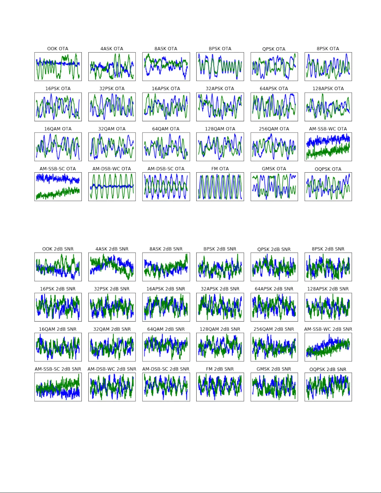
1 Ov er the Air Deep Learning Based Radio Signal Classification T im O’Shea, Senior Member , IEEE, T amoghna Roy , Member , IEEE and T . Charles Clancy , Senior Member , IEEE Abstract —W e conduct an in depth study on the performance of deep learning based radio signal classification f or radio commu- nications signals. W e consider a rigorous baseline method using higher order moments and strong boosted gradient tree classi- fication and compare perf ormance between the two approaches across a range of configurations and channel impairments. W e consider the effects of carrier frequency offset, symbol rate, and multi-path fading in simulation and conduct over -the-air measurement of radio classification performance in the lab using software radios and compare performance and training strategies for both. Finally we conclude with a discussion of remaining problems, and design considerations for using such techniques. I . I N T RO D U C T I O N Rapidly understanding and labeling of the radio spectrum in an autonomous way is a key enabler for spectrum interference monitoring, radio fault detection, dynamic spectrum access, opportunistic mesh networking, and numerous regulatory and defense applications. Boiling down a comple x high-data rate flood of RF information to precise and accurate labels which can be acted on and conv eyed compactly is a critical com- ponent today in numerous radio sensing and communications systems. For many years, radio signal classification and modu- lation recognition have been accomplished by carefully hand- crafting specialized feature extractors for specific signal types and properties and by and deri ving compact decision bounds from them using either analytically deriv ed decision bound- aries or statistical learned boundaries within low-dimensional feature spaces. In the past five years, we ha ve seen rapid disruption oc- curring based on the improv ed neural network architectures, algorithms and optimization techniques collectiv ely kno wn as deep learning (DL) [26]. DL has recently replaced the machine learning (ML) state of the art in computer vision, voice and natural language processing; in both of these fields, feature engineering and pre-processing were once critically important topics, allowing cleverly designed feature extractors and transforms to extract pertinent information into a man- ageable reduced dimension representation from which labels or decisions could be readily learned with tools like support vector machines or decision trees. Among these widely used front-end features were the scale-inv ariant feature transform (SIFT) [9], the bag of words [8], Mel-frequenc y Cepstral coefficients (MFCC) [1] and others which were widely relied Authors are with the Bradley Department of Electrical and Com- puter Engineering, V ir ginia T ech and DeepSig, Arlington, V A e-mail: (os- hea,tamoghna,tcc)@vt.edu. upon only a few years ago, but are no longer needed for state of the art performance today . DL greatly increased the capacity for feature learning di- rectly on raw high dimensional input data based on high lev el supervised objectiv es due to the new found capacity for learn- ing of very large neural network models with high numbers of free parameters. This was made possible by the combination of strong regularization techniques [18], [21], greatly improv ed methods for stochastic gradient descent (SGD) [15], [16], low cost high performance graphics card processing power , and combining of key neural network architecture innov ations such as con volutional neural networks [5], and rectified linear units [13]. It was not until Alexnet [14] that many of these techniques were used together to realize an increase of sev eral orders of magnitude in the practical model size, parameter count, and target dataset and task complexity which made feature learning directly from imagery state of the art. At this point, the trend in ML has been relentless to wards the replacement of rigid simplified analytic features and models with approximate models with much more accurate high degrees of freedom (DOF) models deriv ed from data using end-to-end feature learning. This trend has been demonstrated in vision, text processing, and voice, but has yet to be widely applied or fully realized on radio time series data sets until recently . W e showed in [30], [32] that these methods can be readily applied to simulated radio time series sample data in order to classify emitter types with excellent performance, obtaining equiv alent accuracies sev eral times more sensitiv e than e xisting best practice methods using feature based classifiers on higher order moments. In this work we provide a more extensiv e dataset of additional radio signal types, a more realistic simulation of the wireless propagation en vironment, ov er the air measurement of the new dataset (i.e. real propagation effects), ne w methods for signal classification which drastically outperform those we initially introduced, and an in depth analysis of man y practical engineering design and system parameters impacting the performance and accurac y of the radio signal classifier . I I . B A C K G RO U N D A. Baseline Classification Appr oach 1) Statistical Modulation F eatures: F or digital modulation techniques, higher order statistics and cyclo-stationary mo- ments [2], [3], [10], [23], [33] are among the most widely used features to compactly sense and detect signals with strong periodic components such as are created by the structure of the 2 carrier , symbol timing, and symbol structure for certain mod- ulations. By incorporating precise kno wledge of this structure, expected v alues of peaks in auto-correlation function (A CF) and spectral correlation function (SCF) surfaces have been used successfully to provide robust classification for signals with unknown or purely random data. For analog modulation where symbol timing does not produce these artif acts, other statistical features are useful in performing signal classifica- tion. For our baseline features in this work, we le verage a number of compact higher order statistics (HOSs). T o obtain these we compute the higher order moments (HOMs) using the expression giv en below: M ( p, q ) = E [ x p − q ( x ∗ ) q ] (1) From these HOMs we can deriv e a number of higher order cumulantss (HOCs) which have been sho wn to be effectiv e discriminators for many modulation types [23]. HOCs can be computed combinatorially using HOMs, each expression varying slightly; below we show one example such expression for the C (4 , 0) HOM. C (4 , 0) = q M (4 , 0) − 3 × M (2 , 0) 2 (2) Additionally we consider a number of analog features which capture other statistical beha viors which can be useful, these include mean, standard deviation and kurtosis of the normal- ized centered amplitude, the centered phase, instantaneous frequency , absolute normalized instantaneous frequency , and sev eral others which hav e shown to be useful in prior work. [6]. 2) Decision Criterion: When mapping our baseline features to a class label, a number of compact machine learning or analytic decision processes can be used. Probabilistically deriv ed decision trees on e xpert modulation features were among the first to be used in this field, but for many years such decision processes have also been trained directly on datasets represented in their feature space. Popular methods here include support vector machines (SVMs), decision trees (DT rees), neural networks (NNs) and ensembling methods which combine collections of classifiers to improve perfor- mance. Among these ensembling methods are Boosting, Bag- ging [4], and Gradient tree boosting [7]. In particular , XGBoost [24] has prov en to be an extremely effecti ve implementation of gradient tree boosting which has been used successfully by winners of numerous Kaggle data science competitions [12]. In this work we opt to use the XGBoost approach for our feature classifier as it outperforms any single decision tree, SVM, or other method e valuated consistently as was the case in [32]. B. Radio Channel Models When modeling a wireless channel there are many com- pact stochastic models for propagation effects which can be used [11]. Primary impairments seen in any wireless channel include: • carrier frequency offset (CFO): carrier phase and fre- quency offset due to disparate local oscillators (LOs) and motion (Doppler). • symbol rate offset (SR O): symbol clock offset and time dilation due to disparate clock sources and motion. • Delay Spread: non-impulsiv e delay spread due to de- layed reflection, diffraction and diffusion of emissions on multiple paths. • Thermal Noise: additi ve white-noise impairment at the receiv er due to physical device sensitivity . Each of these ef fects can be compactly modeled well and is present in some form on any wireless propagation medium. There are numerous additional propagation effects which can also be modeled synthetically beyond the scope of our explo- ration here. C. Deep Learning Classification Appr oach DL relies today on SGD to optimize large parametric neural network models. Since Alexnet [14] and the techniques described in section I, there hav e been numerous architectural advances within computer vision leading to significant per- formance improvements. Howe ver , the core approach remains largely unchanged. Neural networks are comprised of a series of layers which map each layer input h 0 to output h 1 using parametric dense matrix operations follo wed by non-linearities. This can be expressed simply as follows, where weights, W , hav e the dimension | h 0 × h 1 | , bias, b, has the dimension | h 1 | (both constituting θ ), and max is applied element-wise per- output | h 1 | (applying rectified linear unit (ReLU) activ ation functions). h 1 = max (0 , h 0 W + b ) (3) Con volutional layers can be formed by assigning a shape to inputs and outputs and forming W from the replication of filter tap variables at regular strides across the input (to reduce parameter count and enforce translation in v ariance). T raining typically lev erages a loss function ( L ), in this case (for supervised classification) categorical cross-entropy , between one-hot known class labels y i (a zero vector , with a one value at the class inde x i of the correct class) and predicted class v alues ˆ y i . L ( y , ˆ y ) = − 1 N N X i =0 [ y i log( ˆ y i ) + (1 − y i ) log(1 − ˆ y i )] (4) Back propagation of loss gradients can be used to iterati vely update network weights ( θ ) for each epoch n within the network ( f ( x, θ ) ) until validation loss is no longer decreasing. W e use the Adam optimizer [16], whose form roughly follows the conv entional SGD expression below , except for a more complex time varying expression for learning rate ( η ) beyond the scope of this work. θ n +1 = θ n − η ∂ L ( y, f ( x, θ n )) ∂ θ n (5) 3 T ABLE I. R A ND O M V A R IA B L E I N I TI A L I ZAT IO N Random V ariable Distribution α U (0 . 1 , 0 . 4) ∆ t U (0 , 16) ∆ f s N (0 , σ clk ) θ c U (0 , 2 π ) ∆ f c N (0 , σ clk ) H Σ i δ ( t − Rayleigh i ( τ )) T o reduce ov er fitting to training data, regularization is used. W e use batch normalization [21] for regularization of con volutional layers and Alpha Dropout [31] for regularization of fully connected layers. Detail descriptions of additional layers used including SoftMax, Max-Pooling, etc are beyond the scope of this work and are described fully in [26]. I I I . D A TA S E T G E N E R AT I O N A P P R OAC H Fig. 1. Fading Power Delay Profile Examples W e generate new datasets for this in vestigation by building upon an improved version of the tools described in [29]. 24 different analog and digital modulators are used which cov er a wide range of single carrier modulation schemes. W e consider sev eral dif ferent propagation scenarios in the conte xt of this work, first are se veral simulated wireless channels generated from the model sho wn in figure 2, and second we consider ov er the air (O T A) transmission channel of clean signals as sho wn in figures 3 and 4 with no synthetic channel impairments. Digital signals are shaped with a root-raised cosine pulse shaping filter [36] with a range of roll-of f values ( α ). For each example in the synthetic data sets, we indepen- dently draw a random v alue for each of the variables shown below in table I. This results in a new and uncorrelated random channel initialization for each example. Figure 1 illustrates sev eral random values for H , the channel impulse response env elope, for different delay spreads, τ = [0 , 0 . 5 , 1 . 0 , 2 . 0] , relating to dif ferent lev els of multi-path fading in increasingly more difficult Rayleigh fading en vironments. Figure 22 illustrate examples from the training set when using a simulated channel at lo w SNR (0 dB E s / N 0 ). W e consider two different compositions of the dataset, first a “Normal” dataset, which consists of 11 classes which are all relatively low information density and are commonly seen in impaired en vironments. These 11 signals represent a relativ ely simple classification task at high SNR in most cases, somewhat comparable to the canonical MNIST digits. Second, we introduce a “Dif ficult” dataset, which contains all 24 modulations. These include a number of high order modulations (QAM256 and APSK256), which are used in the real world in very high-SNR low-fading channel en vironments such as on impulsiv e satellite links [25] (e.g. D VB-S2X). W e howe v er , apply impairments which are beyond that which you would expect to see in such a scenario and consider only relativ ely short-time observation windows for classification, where the number of samples ( ` ) is = 1024 . Short time classification is a hard problem since decision processes can not wait and acquire more data to increase certainty . This is the case in many real world systems when dealing with short observations (such as when rapidly scanning a recei ver) or short signal bursts in the environment. Under these effects, with low SNR examples (from -20 dB to +30 dB E s / N 0 ), one would not expect to be able to achie ve anywhere near 100% classification rates on the full dataset, making it a good benchmark for comparison and future research comparison. The specific modulations considered within each of these two dataset types are as follows: • Normal Classes: OOK, 4ASK, BPSK, QPSK, 8PSK, 16QAM, AM-SSB-SC, AM-DSB-SC, FM, GMSK, OQPSK • Difficult Classes: OOK, 4ASK, 8ASK, BPSK, QPSK, 8PSK, 16PSK, 32PSK, 16APSK, 32APSK, 64APSK, 128APSK, 16QAM, 32QAM, 64QAM, 128QAM, 256QAM, AM-SSB-WC, AM-SSB-SC, AM-DSB-WC, AM-DSB-SC, FM, GMSK, OQPSK The raw datasets will be made av ailable on the RadioML website 1 shortly after publication. A. Over the air data captur e In additional to simulating wireless channel impairments, we also implement an O T A test-bed in which we modulate and transmit signals using a univ ersal software radio peripheral (USRP) [19] B210 software defined radio (SDR). W e use a second B210 (with a separate free-running LO) to receiv e these transmissions in the lab, over a relativ ely benign indoor wireless channel on the 900MHz ISM band. These radios use the Analog De vices AD9361 [35] radio frequency integrated circuit (RFIC) as their radio front-end and have an LO that provides a frequency (and clock) stability of around 2 parts per million (PPM). W e off-tune our signal by around 1 MHz to av oid DC signal impairment associated with direct conv ersion, but store signals at base-band (offset only by LO error). Receiv ed test emissions are stored off unmodified along with ground truth labels for the modulation from the emitter . I V . S I G N AL C L A S S I FI C A T I O N M O D E L S In this section we explore the radio signal classification methods in more detail which we will use for the remainder of this paper . 1 https://radioml.org 4 Fig. 2. System for dataset signal generation and synthetic channel impairment modeling Fig. 3. Over the Air T est Configuration T ABLE II. F E A TU R E S U S E D Feature Name M(2,0), M(2,1) M(4,0), M(4,1), M(4,2), M(4,3) M(6,0), M(6,1), M(6,2), M(6,3) C(2,0), C(2,1) C(4,0), C(4,1), C(4,2), C(6,0), C(6,1), C(6,2), C(6,3) Additional analog II-A A. Baseline Method Our baseline method lev erages the list of higher order moments and other aggregate signal beha vior statistics gi ven in table II. Here we can compute each of these statistics over each 1024 sample example, and translate the example into feature space, a set of real values associated with each statistic for the example. This ne w representation has reduced the dimension of each example from R 1024 ∗ 2 to R 28 , making the classification task much simpler b ut also discarding the v ast majority of the data. W e use an ensemble model of gradient boosted trees (XGBoost) [24] to classify modulations from these features, which outperforms a single decision tree or support vector machine (SVM) significantly on the task. B. Con volutional Neural Network Since [5] and [14] the use of conv olutional neural network (CNN) layers to impart translation in v ariance in the input, Fig. 4. Configuration for Over the Air T ransmission of Signals followed by fully connected layers (FC) in classifiers, has been used in the computer vision problems. In [17], the question of ho w to structure such networks is explored, and se veral basic design principals for ”VGG” networks are introduced (e.g. filter size is minimized at 3x3, smallest size pooling operations are used at 2x2). Following this approach has generally led to straight forward way to construct CNNs with good performance. W e adapt the VGG architecture principals to a 1D CNN, improving upon the similar networks in [30], [32]. This represents a simple DL CNN design approach which can be readily trained and deployed to effecti vely accomplish many small radio signal classification tasks. Of significant note here, is that the features into this CNN are the raw I/Q samples of each radio signal example which hav e been normalized to unit variance. W e do not perform any expert feature extraction or other pre-processing on the raw radio signal, instead allo wing the network to learn raw time- 5 T ABLE III. C N N N E T WO R K L AYO U T Layer Output dimensions Input 2 × 1024 Con v 64 × 1024 Max Pool 64 × 512 Con v 64 × 512 Max Pool 64 × 256 Con v 64 × 256 Max Pool 64 × 128 Con v 64 × 128 Max Pool 64 × 64 Con v 64 × 64 Max Pool 64 × 32 Con v 64 × 32 Max Pool 64 × 16 Con v 64 × 16 Max Pool 64 × 8 FC/Selu 128 FC/Selu 128 FC/Softmax 24 series features directly on the high dimension data. Real valued networks are used, as complex v alued auto-differentiation is not yet mature enough for practical use. C. Residual Neural Network As network algorithms and architectures ha ve improved since Alexnet, they have made the effecti ve training of deeper networks using more and wider layers possible, and leading to improv ed performance. In our original work [30] we employ only a small con volutional neural network with sev eral layers to improve over the prior state of the art. Howe ver in the computer vision space, the idea of deep residual networks has become increasingly effecti ve [27]. In a deep residual network, as is shown in figure 5, the notion of skip or bypass connections is used heavily , allowing for features to operate at multiple scales and depths through the network. This has led to significant improvements in computer vision performance, and has also been used effecti vely on time-series audio data [28]. In [34], the use of residual networks for time-series radio classification is in vestigated, and seen to train in fewer epochs, but not to provide significant performance improv ements in terms of classification accurac y . W e re visit the problem of modulation recognition with a modified residual network and obtain improv ed performance when compared to the CNN on this dataset. The basic residual unit and stack of residual units is sho wn in figure 5, while the network architecture for our best architecture for ( ` = 1024 ) is shown in table IV. W e also employ self-normalizing neural networks [31] in the fully connected region of the network, employing the scaled exponential linear unit (SELU) activ ation function, mean- response scaled initialization (MRSA) [20], and Alpha Dropout [31], which provides a slight improvement ov er con ventional ReLU performance. For the two network layouts shown, with ` = 1024 and L = 5 , The ResNet has 236,344 trainable parameters, while the CNN/VGG network has a comparable 257,099 trainable parameters. V . S E N S I N G P E R F O R M A N C E A N A L Y S I S There are numerous design, deployment, training, and data considerations which can significantly effect the performance Fig. 5. Hierarchical Layers Used in Network T ABLE IV . R E S N E T N ET W O RK L A YO U T Layer Output dimensions Input 2 × 1024 Residual Stack 32 × 512 Residual Stack 32 × 256 Residual Stack 32 × 128 Residual Stack 32 × 64 Residual Stack 32 × 32 Residual Stack 32 × 16 FC/SeLU 128 FC/SeLU 128 FC/Softmax 24 of a DL based approach to radio signal classification which must be carefully considered when designing a solution. In this section we explore sev eral of the most common design parameters which impact classification accuracy including radio propagation effects, model size/depth, data set sizes, observation size, and signal modulation type. A. Classification on Low Or der Modulations W e first compare performance on the lower dif ficulty dataset on lower order modulation types. T raining on a dataset of 1 million example, each 1024 samples long, we obtain excellent performance at high SNR for both the VGG CNN and the ResNet (RN) CNN. In this case, the ResNet achie ves roughly 5 dB higher sensitivity for equiv alent classification accuracy than the base- line, and at high SNR a maximum classification accurac y rate of 99.8% is achieved by the ResNet, while the VGG network achieves 98.3% and the baseline method achie ves a 94.6% accuracy . At lo wer SNRs, performance between VGG and ResNet networks are virtually identical, but at high- SNR performance improv es considerably using the ResNet and obtaining almost perfect classification accuracy . 6 − 20 − 10 0 10 0 0 . 2 0 . 4 0 . 6 0 . 8 1 E s / N 0 [dB] Correct classification probability BL VGG RN Fig. 6. 11-modulation A WGN dataset performance comparison (N=1M) − 20 − 10 0 10 0 0 . 2 0 . 4 0 . 6 0 . 8 1 E s / N 0 [dB] Correct classification probability BL A WGN RN A WGN VGG A WGN Fig. 7. Comparison models under A WGN (N=240k) For the remainder of the paper , we will consider the much harder task of 24 class high order modulations containing higher information rates and much more easily confused classes between multiple high order PSKs, APSKs and QAMs. B. Classification under A WGN conditions Signal classification under additi ve white gaussian noise (A WGN) is the canonical problem which has been e xplored for many years in communications literature. It is a simple starting point, and it is the condition under which analytic feature extractors should generally perform their best (since they were derived under these conditions). In figure 7 we compare the performance of the ResNet (RN), VGG network, and the baseline (BL) method on our full dataset for ` = 1024 − 20 − 10 0 10 0 0 . 2 0 . 4 0 . 6 0 . 8 1 E s / N 0 [dB] Correct classification probability RN A WGN RN σ clk = 0 . 01 RN σ clk = 0 . 0001 RN τ = 0 . 5 RN τ = 1 RN τ = 2 RN τ = 4 Fig. 8. Resnet performance under various channel impairments (N=240k) samples, N = 239 , 616 examples, and L = 6 residual stacks. Here, the residual network provides the best performance at both high and low SNRs on the difficult dataset by a margin of 2-6 dB in improv ed sensitivity for equiv alent classification accuracy . C. Classification under Impairments In any real world scenario, wireless signals are impaired by a number of effects. While A WGN is widely used in simulation and modeling, the effects described abo ve are present almost universally . It is interesting to inspect how well learned classifiers perform under such impairments and compare their rate of de gradation under these impairments with that of more traditional approaches to signal classification. In figure 8 we plot the performance of the residual network based classifier under each considered impairment model. This includes A WGN, σ clk = 0 . 0001 - minor LO of fset, σ clk = 0 . 01 - moderate LO of fset, and sev eral fading models ranging from τ = 0 . 5 to τ = 4 . 0 . Under the fading models, moderate LO of fset is assumed as well. Interestingly in this plot, ResNet performance impro ves under LO offset rather than degrading. Additional LO offset which results in spinning or dilated v ersions of the original signal, appears to hav e a positiv e regularizing effect on the learning process which provides quite a noticeable improv ement in performance. At high SNR performance ranges from around 80% in the best case do wn to about 59% in the worst case. In figure 9 we show the degradation of the baseline classifier under impairments. In this case, LO offset never helps, but the performance instead degrades with both LO of fset and fading effects, in the best case at high SNR this method obtains about 61% accurac y while in the worst case it de grades to around 45% accuracy . Directly comparing the performance of each model under moderate LO impairment effects, in figure 10 we show that 7 − 20 − 10 0 10 0 0 . 2 0 . 4 0 . 6 0 . 8 1 E s / N 0 [dB] Correct classification probability BL A WGN BL σ clk = 0 . 01 BL σ clk = 0 . 0001 BL τ = 0 . 5 BL τ = 1 BL τ = 2 BL τ = 4 Fig. 9. Baseline performance under channel impairments (N=240k) − 20 − 10 0 10 0 0 . 2 0 . 4 0 . 6 0 . 8 1 E s / N 0 [dB] Correct classification probability BL σ clk = 0 . 01 RN σ clk = 0 . 01 VGG σ clk = 0 . 01 Fig. 10. Comparison models under LO impairment for many real world systems with unsynchronized LOs and Doppler frequency of fset there is nearly a 6dB performance advantage of the ResNet approach vs the baseline, and a 20% accuracy increase at high SNR. In this section, all models are trained using N = 239 , 616 and ` = 1024 for this comparison. D. Classifier performance by depth Model size can ha ve a significant impact on the ability of large neural network models to accurately represent complex features. In computer vision, con volutional layer based DL models for the ImageNet dataset started around 10 layers deep, but modern state of the art networks on ImageNet are often ov er 100 layers deep [22], and more recently ev en o ver 200 layers. Initial in vestig ations of deeper networks in [34] did not − 20 − 10 0 10 0 0 . 2 0 . 4 0 . 6 0 . 8 1 E s / N 0 [dB] Correct classification probability L=1 L=2 L=3 L=4 L=5 L=6 Fig. 11. ResNet performance vs depth (L = number of residual stacks) show significant gains from such large architectures, but with use of deep residual networks on this larger dataset, we begin to see quite a benefit to additional depth. This is likely due to the significantly larger number of examples and classes used. In figure 11 we show the increasing validation accuracy of deep residual networks as we introduce more residual stack units within the network architecture (i.e. making the network deeper). W e see that performance steadily increases with depth in this case with diminishing returns as we approach around 6 layers. When considering all of the primitive layers within this network, when L = 6 we the ResNet has 121 layers and 229k trainable parameters, when L = 0 it has 25 layers and 2.1M trainable parameters. Results are shown for N = 239 , 616 and ` = 1024 . E. Classification performance by modulation type In figure 12 we show the performance of the classifier for individual modulation types. Detection performance of each modulation type varies drastically over about 18dB of signal to noise ratio (SNR). Some signals with lower information rates and v astly different structure such as AM and FM analog modulations are much more readily identified at low SNR, while high-order modulations require higher SNRs for robust performance and never reach perfect classification rates. Howe v er , all modulation types reach rates above 80% accuracy by around 10dB SNR. In figure 13 we show a confusion matrix for the classifier across all 24 classes for A WGN validation examples where SNR is greater than or equal to zero. W e can see again here that the lar gest sources of error are between high order phase shift keying (PSK) (16/32-PSK), between high order quadrature amplitude modulation (QAM) (64/128/256-QAM), as well as between AM modes (confusing with-carrier (WC) and suppressed-carrier (SC)). This is largely to be expected as for short time observations, and under noisy observations, high order QAM and PSK can be extremely difficult to tell apart through any approach. 8 − 20 − 15 − 10 − 5 0 5 10 15 0 0 . 1 0 . 2 0 . 3 0 . 4 0 . 5 0 . 6 0 . 7 0 . 8 0 . 9 1 Signal to noise ratio ( E s / N 0 ) [dB] Correct classification probability OOK 4ASK 8ASK BPSK QPSK 8PSK 16PSK 32PSK 16APSK 32APSK 64APSK 128APSK 16QAM 32QAM 64QAM 128QAM 256QAM AM-SSB-WC AM-SSB-SC AM-DSB-WC AM-DSB-SC FM GMSK OQPSK Fig. 12. Modrec performance vs modulation type (Resnet on synthetic data with N=1M, σ clk =0.0001) F . Classifier T raining Size Requir ements When using data-centric machine learning methods, the dataset often has an enormous impact on the quality of the model learned. W e consider the influence of the number of example signals in the training set, N , as well as the time- length of each indi vidual example in number of samples, ` . In figure 14 we show how performance of the resulting model changes based on the total number of training examples used. Here we see that dataset size has a dramatic impact on model training, high SNR classification accuracy is near random until 4-8k examples and improves 5-20% with each doubling until around 1M. These results illustrate that having sufficient training data is critical for performance. For the largest case, with 2 million examples, training on a single state of the art Nvidia V100 graphics processing unit (GPU) (with approximately 125 tera-floating point operations per second (FLOPS)) takes around 16 hours to reach a stopping point, making significant experimentation at these dataset sizes cum- bersome. W e do not see significant impro vement going from 1M to 2M examples, indicating a point of diminishing returns for number of examples around 1M with this configuration. W ith either 1M or 2M examples we obtain roughly 95% test set accuracy at high SNR. The class-confusion matrix for the best performing mode with ` =1024 and N=1M is shown in figure 15 for test examples at or above 0dB SNR, in all instances here we use the σ clk = 0 . 0001 dataset, which yields slightly better performance than A WGN. Figure 16 sho ws how the model performance v aries by window size, or the number of time-samples per example used for a single classification. Here we obtain approximately a 3% accuracy improvement for each doubling of the input size (with N=240k), with significant diminishing returns once we reach ` = 512 or ` = 1024 . W e find that CNNs scale very well up to this 512-1024 size, but may need additional scaling strategies thereafter for larger input windows simply due to memory requirements, training time requirements, and dataset requirements. G. Over the air performance W e generate 1.44M examples of the 24 modulation dataset ov er the air using the USRP setup described above. Using a partition of 80% training and 20% test, we can directly train a ResNet for classification. Doing so on an Nvidia V100 in around 14 hours, we obtain a 95.6% test set accuracy on the ov er the air dataset, where all e xamples are roughly 10dB SNR. 9 Fig. 13. 24-modulation confusion matrix for ResNet trained and tested on synthetic dataset with N=1M and A WGN − 20 − 10 0 10 0 0 . 2 0 . 4 0 . 6 0 . 8 1 E s / N 0 [dB] Correct classification probability N=1k N=2k N=4k N=8k N=15k N=31k N=62k N=125k N=250k N=500k N=1M N=2M Fig. 14. Performance vs training set size (N) with ` = 1024 A confusion matrix for this O T A test set performance based on direct training is sho wn in figure 17. H. T r ansfer learning over -the-air performance W e also consider ov er the air signal classification as a trans- fer learning problem, where the model is trained on synthetic data and then only ev aluated and/or fine-tuned on O T A data. Because full model training can take hours on a high end GPU and typically requires a large dataset to be effecti ve, transfer learning is a conv enient alternative for le v eraging e xisting models and updating them on smaller computational platforms and tar get datasets. W e consider transfer learning, where we freeze network parameter weights for all layers except the Fig. 15. 24-modulation confusion matrix for ResNet trained and tested on synthetic dataset with N=1M and σ clk = 0 . 0001 − 20 − 10 0 10 0 0 . 2 0 . 4 0 . 6 0 . 8 1 E s / N 0 [dB] Correct classification probability ` =16 ` =32 ` =64 ` =128 ` =256 ` =512 ` =768 ` =1024 Fig. 16. Performance vs example length in samples ( ` ) last several fully connected layers (last three layers from table IV) in our network when while updating. This is commonly done today with computer vision models where it is common start by using pre-trained VGG or other model weights for ImageNet or similar datasets and perform transfer learning using another dataset or set of classes. In this case, many low- lev el features w ork well for dif ferent classes or datasets, and do not need to change during fine tuning. In our case, we consider sev eral cases where we start with models trained on simulated wireless impairment models using residual networks and then ev aluate them on O T A examples. The accuracies of our initial models (trained with N=1M) on synthetic data shown in figure 8, and these ranged from 84% to 96% on the hard 24-class 10 Fig. 17. 24-modulation confusion matrix for ResNet trained and tested on O T A examples with SNR ∼ 10 dB 10 20 30 40 50 0 . 6 0 . 7 0 . 8 0 . 9 T ransfer Learning Epochs Correct classification probability (T est Set) A WGN σ clk =0.0001 σ clk =0.01 τ = 0.5 τ = 1.0 Fig. 18. RESNET T ransfer Learning OT A Performance (N=120k) dataset. Ev aluating performance of these models on O T A data, without any model updates, we obtain classification accuracies between 64% and 80%. By fine-tuning the last two layers of these models on the O T A data using transfer learning, we and can recov er approximately 10% of additional accuracy . The validation accuracies are shown for this process in figure 18. These ResNet update epochs on dense layers for 120k examples take roughly 60 seconds on a Titan X card to execute instead of the full ∼ 500 seconds on V100 card per epoch when updating model weights. Ultimately , the model trained on just moderate LO offset ( σ clk = 0.0001) performs the best on OT A data. The model obtained 94% accurac y on synthetic data, and drops roughly Fig. 19. 24-modulation confusion matrix for ResNet trained on synthetic σ clk = 0 . 0001 and tested on OT A examples with SNR ∼ 10 dB (prior to fine-tuning) Fig. 20. 24-modulation confusion matrix for ResNet trained on synthetic σ clk = 0 . 0001 and tested on OT A examples with SNR ∼ 10 dB (after fine- tuning) 7% accurac y when e v aluating on O T A data, obtaining an accuracy of 87%. The primary confusion cases prior to training seem to be dealing with suppress or non-suppressed carrier analog signals, as well as the high order QAM and APSK modes. This seems like it is perhaps the best suited among our models to match the O T A data. V ery small LO impairments are present in the data, the radios used had extremely stable oscillators present (GPSDO modules providing high stable ˜ 75 PPB clocks) over very short example lengths (1024 samples), REFERENCES 11 and that the two radios were essentially right next to each other , providing a very clean impulsiv e direct path while any reflections from the surrounding room were likely significantly attenuated in comparison, making for a near impulsi ve channel. T raining on harsher impairments seemed to degrade perfor- mance of the O T A data significantly . W e suspect as we ev aluate the performance of the model under increasingly harsh real w orld scenarios, our transfer learning will fav or synthetic models which are similarly im- paired and most closely match the real wireless conditions (e.g. matching LO distributions, matching fading distributions, etc). In this way , it will be important for this class of systems to train either directly on tar get signal en vironments, or on very good impairment simulations of them under which well suited models can be deri ved. Possible mitigation to this are to include domain-matched attention mechanisms such as the radio transformer network [29] in the network architecture to improv e generalization to varying wireless propagation conditions. V I . D I S C U S S I O N In this work we have extended prior work on using deep con volutional neural networks for radio signal classification by heavily tuning deep residual netw orks for the same task. W e hav e also conducted a much more thorough set of performance ev aluations on how this type of classifier performs o ver a wide range of design parameters, channel impairment condi- tions, and training dataset parameters. This residual netw ork approach achie ves state of the art modulation classification per - formance on a dif ficult new signal database both synthetically and in over the air performance. Other architectures still hold significant potential, radio transformer networks, recurrent units, and other approaches all still need to be adapted to the domain, tuned and quantitativ ely benchmarked against the same dataset in the future. Other works hav e explored these to some degree, b ut generally not with suf ficient hyper -parameter optimization to be meaningful. W e hav e shown that, contrary to prior work, deep networks do provide significant performance gains for time-series radio signals where the need for such deep feature hierarchies was not apparent, and that residual networks are a highly effecti ve way to build these structures where more traditional CNNs such as VGG struggle to achieve the same performance or make effecti ve use of deep networks. W e ha ve also shown that simulated channel effects, especially moderate LO impair- ments improv e the effect of transfer learning to OT A signal ev aluation performance, a topic which will require significant future inv estigation to optimize the synthetic impairment dis- tributions used for training. V I I . C O N C L U S I O N DL methods continue to sho w enormous promise in im- proving radio signal identification sensitivity and accurac y , especially for short-time observations. W e hav e shown deep networks to be increasingly effecti ve when le veraging deep residual architectures and hav e shown that synthetically trained deep networks can be effecti vely transferred to ov er the air datasets with (in our case) a loss of around 7% accuracy or directly trained effecti vely on O T A data if enough training data is av ailable. While large well labeled datasets can often be difficult to obtain for such tasks today , and channel models can be difficult to match to real-world deployment conditions, we hav e quantified the real need to do so when training such systems and helped quantify the performance impact of doing so. W e still hav e much to learn about ho w to best curate datasets and training regimes for this class of systems. Howe ver , we hav e demonstrated in this work that our approach provides roughly the same performance on high SNR O T A datasets as it does on the equi valent synthetic datasets, a major step tow ards real world use. W e have demonstrated that transfer learning can be effecti ve, but have not yet been able to achiev e equiv alent performance to direct training on very large datasets by using transfer learning. As simulation methods become better , and our ability to match synthetic datasets to real world data distributions improv es, this gap will close and transfer learning will become and increasingly important tool when real data capture and labeling is difficult. The performance trades shown in this work help shed light on these ke y parameters in data generation and training, hopefully helping increase understanding and focus future efforts on the optimization of such systems. R E F E R E N C E S [1] S. Imai, “Cepstral analysis synthesis on the mel fre- quency scale, ” in Acoustics, Speech, and Signal Pr o- cessing, IEEE International Conference on ICASSP’83. , IEEE, vol. 8, 1983, pp. 93–96. [2] W . A. Gardner and C. M. Spooner, “Signal interception: Performance advantages of cyclic-feature detectors, ” IEEE T ransactions on Communications , vol. 40, no. 1, pp. 149–159, 1992. [3] C. M. Spooner and W . A. Gardner , “Robust feature detection for signal interception, ” IEEE transactions on communications , vol. 42, no. 5, pp. 2165–2173, 1994. [4] J. R. Quinlan et al. , “Bagging, boosting, and c4. 5, ” in AAAI/IAAI, V ol. 1 , 1996, pp. 725–730. [5] Y . LeCun, L. Bottou, Y . Bengio, and P . Haf fner, “Gradient-based learning applied to document recog- nition, ” Pr oceedings of the IEEE , v ol. 86, no. 11, pp. 2278–2324, 1998. [6] A. K. Nandi and E. E. Azzouz, “ Algorithms for au- tomatic modulation recognition of communication sig- nals, ” IEEE T r ansactions on communications , vol. 46, no. 4, pp. 431–436, 1998. [7] J. H. Friedman, “Greedy function approximation: A gra- dient boosting machine, ” Annals of statistics , pp. 1189– 1232, 2001. [8] M. V idal-Naquet and S. Ullman, “Object recognition with informati ve features and linear classification., ” in ICCV , vol. 3, 2003, p. 281. [9] D. G. Lowe, “Distinctiv e image features from scale- in v ariant keypoints, ” International journal of computer vision , vol. 60, no. 2, pp. 91–110, 2004. 12 [10] A Fehske, J Gaeddert, and J. H. Reed, “A new ap- proach to signal classification using spectral correlation and neural networks, ” in New F rontier s in Dynamic Spectrum Access Networks, 2005. DySP AN 2005. 2005 F irst IEEE International Symposium on , IEEE, 2005, pp. 144–150. [11] A. Goldsmith, W ir eless communications . Cambridge univ ersity press, 2005. [12] A. Goldbloom, “Data prediction competitions–far more than just a bit of fun, ” in Data Mining W orkshops (ICDMW), 2010 IEEE International Conference on , IEEE, 2010, pp. 1385–1386. [13] V . Nair and G. E. Hinton, “Rectified linear units im- prov e restricted boltzmann machines, ” in Pr oceedings of the 27th international confer ence on machine learning (ICML-10) , 2010, pp. 807–814. [14] A. Krizhevsk y, I. Sutskev er, and G. E. Hinton, “Ima- genet classification with deep conv olutional neural net- works, ” in Advances in neural information pr ocessing systems , 2012, pp. 1097–1105. [15] T . T ieleman and G. Hinton, “Lecture 6.5-rmsprop: Di- vide the gradient by a running av erage of its recent magnitude, ” COURSERA: Neural networks for machine learning , vol. 4, no. 2, pp. 26–31, 2012. [16] D. Kingma and J. Ba, “Adam: A method for stochastic optimization, ” ArXiv preprint , 2014. [17] K. Simonyan and A. Zisserman, “Very deep con v o- lutional netw orks for large-scale image recognition, ” ArXiv pr eprint arXiv:1409.1556 , 2014. [18] N. Sri vasta v a, G. E. Hinton, A. Krizhe vsky, I. Sutsk ev er, and R. Salakhutdinov , “Dropout: A simple w ay to prev ent neural networks from overfitting., ” J ournal of Machine Learning Researc h , vol. 15, no. 1, pp. 1929– 1958, 2014. [19] M. Ettus and M. Braun, “The uni versal software radio peripheral (usrp) f amily of lo w-cost sdrd, ” Opportunistic Spectrum Sharing and White Space Access: The Prac- tical Reality , pp. 3–23, 2015. [20] K. He, X. Zhang, S. Ren, and J. Sun, “Delving deep into rectifiers: Surpassing human-le vel performance on imagenet classification, ” in Proceedings of the IEEE international conference on computer vision , 2015, pp. 1026–1034. [21] S. Ioffe and C. Szegedy, “Batch normalization: Ac- celerating deep network training by reducing internal cov ariate shift, ” in International Confer ence on Machine Learning , 2015, pp. 448–456. [22] C. Szegedy, W . Liu, Y . Jia, P . Sermanet, S. Reed, D. Anguelov, D. Erhan, V . V anhoucke, and A. Rabinovich, “Going deeper with con v olutions, ” in Pr oceedings of the IEEE confer ence on computer vision and pattern r ecognition , 2015, pp. 1–9. [23] A. Abdelmutalab, K. Assaleh, and M. El-T arhuni, “ Au- tomatic modulation classification based on high or- der cumulants and hierarchical polynomial classifiers, ” Physical Communication , vol. 21, pp. 10–18, 2016. [24] T . Chen and C. Guestrin, “Xgboost: A scalable tree boosting system, ” in Pr oceedings of the 22nd acm sigkdd international confer ence on knowledge discovery and data mining , A CM, 2016, pp. 785–794. [25] S. Cioni, G. Cola volpe, V . Mignone, A. Modenini, A. Morello, M. Ricciulli, A. Ugolini, and Y . Zanettini, “T ransmission parameters optimization and recei ver ar- chitectures for dvb-s2x systems, ” International J ournal of Satellite Communications and Networking , vol. 34, no. 3, pp. 337–350, 2016. [26] I. Goodfellow , Y . Bengio, and A. Courville, Deep learn- ing . MIT press, 2016. [27] K. He, X. Zhang, S. Ren, and J. Sun, “Deep residual learning for image recognition, ” in Pr oceedings of the IEEE conference on computer vision and pattern reco g- nition , 2016, pp. 770–778. [28] A. v . d. Oord, S. Dieleman, H. Zen, K. Simonyan, O. V inyals, A. Gra ves, N. Kalchbrenner, A. Senior, and K. Kavukcuoglu, “Wav enet: A generative model for raw audio, ” ArXiv preprint , 2016. [29] T . J. O’Shea and N. W est, “Radio machine learning dataset generation with gnu radio, ” in Pr oceedings of the GNU Radio Confer ence , vol. 1, 2016. [30] T . J. OShea, J. Corgan, and T . C. Clancy, “Con volu- tional radio modulation recognition networks, ” in In- ternational Conference on Engineering Applications of Neural Networks , Springer, 2016, pp. 213–226. [31] G. Klambauer, T . Unterthiner, A. Mayr, and S. Hochre- iter , “Self-normalizing neural networks, ” ArXiv preprint arXiv:1706.02515 , 2017. [32] T . OShea and J. Hoydis, “An introduction to deep learning for the physical layer, ” IEEE T ransactions on Cognitive Communications and Networking , 2017. [33] C. M. Spooner, A. N. Mody, J. Chuang, and J. Petersen, “Modulation recognition using second-and higher-order cyclostationarity , ” in Dynamic Spectrum Access Net- works (DySP AN), 2017 IEEE International Symposium on , IEEE, 2017, pp. 1–3. [34] N. E. W est and T . J. O’Shea, “Deep architectures for modulation recognition, ” in IEEE International Sym- posium on Dynamic Spectrum Access Networks , IEEE, 2017. [35] A. D.-R.A. T . AD9361, “Url: Https://tinyurl.com/hwxym94 (visited on 09/14/08), ” Cited on , p. 103, [36] J. G. Proakis, “Digital communications. 1995, ” McGraw-Hill, New Y ork , A P P E N D I X 13 Fig. 21. I/Q time domain examples of 24 modulations over the air at roughly 10 dB E s / N 0 ( ` = 256 ) Fig. 22. I/Q time domain examples of 24 modulations from synthetic σ clk = 0 . 01 dataset at 2dB E s / N 0 ( ` = 256 )