DeepSurv: Personalized Treatment Recommender System Using A Cox Proportional Hazards Deep Neural Network

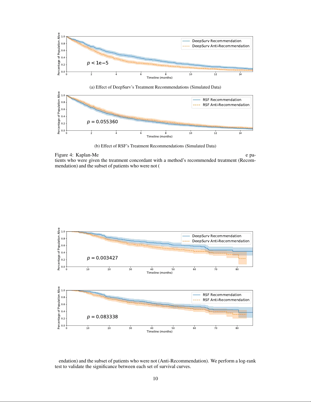
DeepSurv: P ersonalized T r eatment Recommender System Using A Cox Pr oportional Hazards Deep Neural Network Jar ed L. Katzman 1 , Uri Shaham 2,5 , Alexander Cloninger 3,8 , Jonathan Bates 3,4,5 , Tingting Jiang 6 , and Y uval Kluger 3,6,7 1 Department of Computer Science, Y ale Univ ersity , 51 Prospect Steet, New Ha ven, CT 06511, USA 2 Department of Statistics, Y ale Univ ersity , 24 Hillhouse A venue, Ne w Ha ven, CT 06511, USA 3 Applied Mathematics Program, Y ale Univ ersity , 51 Prospect Steet, New Ha ven, CT 06511, USA 4 Y ale School of Medicine, 333 Cedar Street, New Ha ven CT 06510, USA 5 Center for Outcomes Research and Evaluation, Y ale-Ne w Ha ven Hospital, Ne w Haven, CT 6 Interdepartmental Program in Computational Biology and Bioinformatics, Y ale Univ ersity , New Hav en, CT 06511, USA 7 Department of Pathology and Y ale Cancer Center , Y ale Uni versity School of Medicine, Ne w Hav en, CT , USA 8 Department of Mathematics, Univ ersity of California, San Die go, La Jolla, CA 92093, USA Abstract Medical practitioners use surviv al models to explore and understand the rela- tionships between patients’ cov ariates (e.g. clinical and genetic features) and the effecti veness of various treatment options. Standard surviv al models like the linear Cox proportional hazards model require e xtensiv e feature engineering or prior medical knowledge to model treatment interaction at an individual level. While nonlinear surviv al methods, such as neural networks and surviv al forests, can inherently model these high-le vel interaction terms, they have yet to be shown as effecti ve treatment recommender systems. W e introduce DeepSurv , a Cox proportional hazards deep neural network and state-of-the-art survi val method for modeling interactions between a patient’ s cov ariates and treatment ef fecti veness in order to provide personalized treatment recommendations. W e perform a number of experiments training DeepSurv on simulated and real survi v al data. W e demonstrate that DeepSurv performs as well as or better than other state-of-the-art surviv al models and validate that DeepSurv successfully models increasingly comple x relationships between a patient’ s covariates and their risk of failure. W e then show how DeepSurv models the relationship between a patient’ s features and effecti veness of different treatment options to show how DeepSurv can be used to provide individual treatment recommendations. Finally , we train DeepSurv on real clinical studies to demonstrate how it’ s personalized treatment recommendations would increase the surviv al time of a set of patients. The predictiv e and modeling capabilities of DeepSurv will enable medical researchers to use deep neural networks as a tool in their exploration, understanding, and prediction of the effects of a patient’ s characteristics on their risk of failure. 1 Intr oduction Medical researchers use surviv al models to e valuate the significance of prognostic variables in out- comes such as death or cancer recurrence and subsequently inform patients of their treatment options [1, 2, 3, 4]. One standard survi val model is the Cox proportional hazards model (CPH) [5]. The CPH is a semiparametric model that calculates the ef fects of observed co variates on the risk of an ev ent occurring (e.g. ‘death’). The model assumes that a patient’ s risk of failure is a linear combination of the patient’ s co v ariates. This assumption is referred to as the linear pr oportional hazar ds condi- tion. Howe ver , in many applications, such as providing personalized treatment recommendations, it may be too simplistic to assume that the risk function is linear . As such, a richer family of survi v al models is needed to better fit surviv al data with nonlinear risk functions. T o model nonlinear survi v al data, researchers have applied three main types of neural networks to the problem of survi v al analysis. These include variants of: (i) classification methods [see details in 6, 7], (ii) time-encoded methods [see details in 8, 9], (iii) and risk-predicting methods [see details in 10]. This third type is a feed-forward neural network (NN) that estimates an indi vidual’ s risk of failure. In fact, Faraggi-Simon’ s network is seen as a nonlinear extension of the Cox proportional hazards model. Risk neural networks learn highly comple x and nonlinear relationships between prognostic features and an indi vidual’ s risk of failure. In application, for example, when the success of a treatment option is affected by an individual’ s features, the NN learns the relationship without prior feature selection or domain expertise. The network is then able to provide a personalized recommendation based on the computed risk of a treatment. Howe ver , previous studies ha v e demonstrated mixed results on NNs ability to predict risk. F or instance, researchers have attempted to apply the Faraggi-Simon network with various extensions, but they have failed to demonstrate impro vements beyond the linear Cox model, see [11], [12] and [13]. One possible explanation is that the practice of NNs was not as dev eloped as it is today . T o the best of our kno wledge, NNs hav e not outperformed standard methods for surviv al analysis (e.g. CPH). Our manuscript shows that this is no longer the case; with modern techniques, risk NNs ha ve state-of-the-art performance and can be used for a variety of medical applications. The goals of this paper are: (i) to show that the application of deep learning to surviv al analysis performs as well as or better than other survi v al methods in predicting risk; and (ii) to demonstrate that the deep neural network can be used as a personalized treatment recommender system and a useful framew ork for further medical research. W e propose a modern Cox proportional hazards deep neural network, henceforth referred to as DeepSurv , as the basis for a treatment recommender system. W e make the follo wing contributions. First, we show that DeepSurv performs as well as or better than other surviv al analysis methods on surviv al data with both linear and nonlinear risk functions. Second, we include an additional categorical variable representing a patient’ s treatment group to illustrate how the netw ork can learn complex relationships between an individual’ s co variates and the ef fect of a treatment. Our experi- ments v alidate that the network successfully models the treatment’ s risk within a population. Third, we use DeepSurv to provide treatment recommendations tailored to a patient’ s observed features. W e confirm our results on real clinical studies, which further demonstrates the power of DeepSurv . Finally , we show that the recommender system supports medical practitioners in providing person- alized treatment recommendations that potentially could increase the median survi v al time for a set of patients. The or ganization of the manuscript is as follo ws: in Section 2, we provide a brief background on surviv al analysis. In Section 3, we present our contributions, including an explanation of our implementation of DeepSurv and our proposed recommender system. In Section 4, we describe the experimental design and results. Section 5 concludes the manuscript. 2 Backgr ound In this section, we define survi val data and the approaches for modeling a population’ s surviv al and failure rate. Additionally , we discuss linear and nonlinear surviv al models and their limitations. 2.1 Surviv al data Surviv al data is comprised of three elements: a patient’ s baseline data x , a failure ev ent time T , and an event indicator E . If an event (e.g. death) is observed, the time interval T corresponds to the time elapsed between the time in which the baseline data was collected and the time of the 2 ev ent occurring, and the event indicator is E = 1 . If an event is not observed, the time interval T corresponds to the time elapsed between the collection of the baseline data and the last contact with the patient (e.g. end of study), and the event indicator is E = 0 . In this case, the patient is said to be right-censor ed . If one opts to use standard re gression methods, the right-censored data is considered to be a type of missing data. This is typically discarded which can introduce a bias in the model. Therefore, modeling right-censored data requires special consideration or the use of a surviv al model. Surviv al and hazard functions are the two fundamental functions in survi v al analysis. The surviv al function is denoted by S ( t ) = Pr( T > t ) , which signifies the probability that an individual has ‘surviv ed’ beyond time t . The hazard function is a measure of risk at time t . A greater hazard signifies a greater risk of death. The hazard function λ ( t ) is defined as: λ ( t ) = lim δ → 0 Pr( t ≤ T < t + δ | T ≥ t ) δ . (1) A proportional hazards model is a common method for modeling an indi vidual’ s surviv al gi ven their baseline data x . The model assumes that the hazard function is composed of two functions: a baseline hazard function, λ 0 ( t ) , and a risk function, h ( x ) , denoting the effects of an individual’ s cov ariates. The hazard function is assumed to hav e the form λ ( t | x ) = λ 0 ( t ) · e h ( x ) . 2.2 Linear Surviv al Models The CPH is a proportional hazards model that estimates the risk function h ( x ) by a linear function ˆ h β ( x ) = β T x . T o perform Cox regression, one tunes the weights β to optimize the Cox partial likelihood. The partial likelihood is the product of the probability at each ev ent time T i that the ev ent has occurred to individual i , gi ven the set of indi viduals still at risk at time T i . The Cox partial likelihood is parameterized by β and defined as L c ( β ) = Y i : E i =1 exp( ˆ h β ( x i )) P j ∈< ( T i ) exp( ˆ h β ( x j )) , (2) where the v alues T i , E i , and x i are the respecti ve ev ent time, ev ent indicator, and baseline data for the i th observation. The product is defined ov er the set of patients with an observable e vent E i = 1 . The risk set < ( t ) = { i : T i ≥ t } is the set of patients still at risk of f ailure at time t . In man y applications, for e xample modeling nonlinear gene interactions, we cannot assume the data satisfies the linear proportional hazards condition. In this case, the CPH model would require computing high-lev el interaction terms. This becomes prohibitiv ely expensi ve as the number of features and interactions increases. Therefore, a more complex nonlinear model is needed. 2.3 Nonlinear surviv al models The Faraggi-Simon method is a feed-forward neural network that provides the basis for a nonlinear proportional hazards model. [10] experimented with a single hidden layer network with two or three nodes. Their model requires no prior assumption of the risk function h ( x ) other than continuity . Instead, the NN computes nonlinear features from the training data and calculates their linear com- bination to estimate the risk function. Similar to Cox regression, the network optimizes a modified Cox partial likelihood. They replace the linear combination of features ˆ h β ( x ) in Equation 2 with the output of the network ˆ h θ ( x ) . As previous research suggests, the Faraggi-Simon network has not been sho wn to outperform the linear CPH [10, 12, 13]. Furthermore, to the best of our knowledge, we were the first to attempt applying modern deep learning techniques to the Cox proportional hazards loss function. Another popular machine learning approach to modeling patients’ risk function is the random sur- viv al forest (RSF) [14, 15]. The random surviv al forest is a tree method that produces an ensemble estimate for the cumulativ e hazard function. A more recent deep learning approach models the ev ent time according to a W eibull distrib ution with parameters giv en by latent v ariables generated by a deep exponential f amily [16]. 3 3 Methods In this section, we describe our methodology for providing personalized treatment recommendations using DeepSurv . First, we describe the architecture and training details of DeepSurv , an open source Python module that applies recent deep learning techniques to a nonlinear Cox proportional hazards network. Second, we define DeepSurv as a prognostic model and show how to use the network’ s predicted risk function to provide personalized treatment recommendations. 3.1 DeepSurv DeepSurv is a multi-layer perceptron, which predicts a patient’ s risk of death. The output of the network is a single node, which estimates the risk function ˆ h θ ( x ) parameterized by the weights of the network θ . Similar to the Faraggi-Simon netw ork, we set the loss function to be the ne gati ve log partial likelihood of Equation 2: l ( θ ) := − X i : E i =1  ˆ h θ ( x i ) − log X j ∈< ( T i ) e ˆ h θ ( x j )  . (3) W e allo w a deep architecture (i.e. more than one hidden layer) and apply modern techniques such as weight decay re gularization, Rectified Linear Units (ReLU) [17] with batch normalization [18], Scaled Exponential Linear Units (SELU) [19], dropout [20], gradient descent optimization algo- rithms (Stochastic Gradient Descent and Adaptiv e Moment Estimation (Adam) [21]), Nesterov mo- mentum [22], gradient clipping [23], and learning rate scheduling [24]. T o tune the network’ s hyper-parameters, we perform a Random hyper -parameter optimization search [25]. For more technical details, see Appendix A. 3.2 T reatment recommender system In a clinical study , patients are subject to different le vels of risk based on their relev ant prognostic features and which treatment they undergo. W e generalize this assumption as follo ws. Let all patients in a given study be assigned to one of n treatment groups τ ∈ { 0 , 1 , ..., n − 1 } . W e assume each treatment i to have an independent risk function h i ( x ) . Collecti vely , the hazard function becomes: λ ( t ; x | τ = i ) = λ 0 ( t ) · e h i ( x ) . (4) For any patient, the netw ork should be able to accurately predict the risk h i ( x ) of being prescribed a giv en treatment i . Then, based on the assumption that each indi vidual has the same baseline hazard function λ 0 ( t ) , we can take the log of the hazards ratio to calculate the personal risk of prescribing one treatment option over another . W e define this difference of log hazards as the r ecommender function or rec ij ( x ) : rec ij ( x ) = log  λ ( t ; x | τ = i ) λ ( t ; x | τ = j )  = log  λ 0 ( t ) · e h i ( x ) λ 0 ( t ) · e h j ( x )  = h i ( x ) − h j ( x ) . (5) The recommender function can be used to provide personalized treatment recommendations. W e first pass a patient through the network once in treatment group i and again in treatment group j and take the difference. When a patient receives a positive recommendation rec ij ( x ) , treatment i leads to a higher risk of death than treatment j . Hence, the patient should be prescribed treatment j . Conv ersely , a neg ativ e recommendation indicates that treatment i is more ef fecti ve and leads to a lower risk of death than treatment j , and we recommend treatment i . DeepSurv’ s architecture holds an adv antage over the CPH because it calculates the recommender function without an a priori specification of treatment interaction terms. In contrast, the CPH model computes a constant recommender function unless treatment interaction terms are added to the model, see Appendix B for more details. Discov ering relev ant interaction terms is expensiv e because it requires extensi ve e xperimentation or prior biological knowledge of treatment outcomes. Therefore, DeepSurv is more cost-effecti ve compared to CPH. 4 4 Results W e perform four sets of e xperiments: (i) simulated survi v al data, (ii) real surviv al data, (iii) simu- lated treatment data, and (iv) real treatment data. First, we use simulated data to show how DeepSurv successfully learns the true risk function of a population. Second, we validate the network’ s predic- tiv e ability by training DeepSurv on real survi val data. Third, we simulate treatment data to verify that the network models multiple risk functions in a population based on the specific treatment a pa- tient undergoes. F ourth, we demonstrate ho w DeepSurv provides treatment recommendations and show that DeepSurv’ s recommendations improve a population’ s survi v al rate. For more technical details on the experiments, see Appendix A. In addition to training DeepSurv on each dataset, we run a linear CPH regression for a baseline comparison. W e also fit a RSF to compare DeepSurv against a state-of-the-art nonlinear surviv al model. Even though we can compare the RSF’ s predictiv e accurac y to DeepSurv’ s, we do not measure the RSF’ s performance on modeling a simulated dataset’ s true risk function h ( x ) . This is due to the fact that the the RSF calculates the cumulativ e hazard function Λ( t ) = R t 0 λ ( τ ) dτ rather than the hazard function λ ( t ) . 4.1 Evaluation Surviv al data T o ev aluate the models’ predicti ve accuracy on the survi v al data, we measure the concordance-index (C-index) c as outlined by [26]. The C-index is the most common metric used in surviv al analysis and reflects a measure of how well a model predicts the ordering of patients’ death times. For context, a c = 0 . 5 is the av erage C-index of a random model, whereas c = 1 is a perfect ranking of death times. W e perform bootstrapping [27] and sample the test set with replacement to obtain confidence intervals. T able 1: Experimental Results for All Experiments: C-index (95% Confidence Interval) Experiment CPH DeepSurv RSF Simulated Linear 0 . 773677 ( 0 . 772 , 0 . 775 ) 0 . 774019 ( 0 . 772 , 0 . 776 ) 0 . 764925 ( 0 . 763 , 0 . 766 ) Simulated Non- linear 0 . 506951 ( 0 . 505 , 0 . 509 ) 0 . 648902 ( 0 . 647 , 0 . 651 ) 0 . 645540 ( 0 . 643 , 0 . 648 ) WHAS 0 . 817620 ( 0 . 814 , 0 . 821 ) 0 . 862620 ( 0 . 859 , 0 . 866 ) 0 . 893623 ( 0 . 891 , 0 . 896 ) SUPPOR T 0 . 582870 ( 0 . 581 , 0 . 585 ) 0 . 618308 ( 0 . 616 , 0 . 620 ) 0 . 613022 ( 0 . 611 , 0 . 615 ) MET ABRIC 0 . 630618 ( 0 . 627 , 0 . 635 ) 0 . 643374 ( 0 . 639 , 0 . 647 ) 0 . 624331 ( 0 . 620 , 0 . 629 ) Simulated T reat- ment 0 . 481540 ( 0 . 480 , 0 . 483 ) 0 . 582774 ( 0 . 580 , 0 . 585 ) 0 . 569870 ( 0 . 568 , 0 . 572 ) Rotterdam & GBSG 0 . 657750 ( 0 . 654 , 0 . 661 ) 0 . 668402 ( 0 . 665 , 0 . 671 ) 0 . 651190 ( 0 . 648 , 0 . 654 ) T reatment recommendations W e determine the recommended treatment for each patient in the test set using DeepSurv and the RSF . W e do not calculate the recommended treatment for CPH; without preselected treatment- interaction terms, the CPH model will compute a constant recommender function and recommend the same treatment option for all patients. This would ef fecti vely be comparing the survi v al rates between the control and experimental groups. DeepSurv and the RSF are capable of predicting an individual’ s risk per treatment because each computes relev ant interaction terms. For DeepSurv , we choose the recommended treatment by calculating the recommender function (Equation 5). Because the RSF predicts a cumulati ve hazard for each patient, we choose the treatment with the minimum cumulativ e hazard. 5 Once we determine the recommended treatment, we identify two subsets of patients: those whose treatment group aligns with the model’ s recommended treatment (Recommendation) and those who do not undergo the recommended treatment (Anti-Recommendation). W e calculate the median sur - viv al time of each subset to determine if a model’ s treatment recommendations increase the surviv al rate of the patients. W e then perform a log-rank test to validate whether the dif ference between the two subsets is significant. T able 2: Experimental Results for T reatment Recommendations: Median Surviv al T ime (months) Experiment DeepSurv RSF Rec Anti-Rec Rec Anti-Rec Simulated 4 . 069 2 . 827 3 . 116 3 . 625 Rotterdam & GBSG 40 . 099 31 . 770 36 . 567 32 . 394 4.2 Simulated surviv al data In this section, we perform two experiments with simulated surviv al data: one with a linear risk func- tion and one with a nonlinear (Gaussian) risk function. The advantage of using simulated datasets is that we can ascertain whether DeepSurv can successfully model the true risk function instead of ov erfitting random noise. For each experiment, we generate a training, validation, and testing set of N = 4000 , 1000 , 1000 observations respectively . Each observ ation represents a patient vector with d = 10 covariates, each drawn from a uniform distribution on [ − 1 , 1) . W e generate the death time T according to an exponential Cox model [28]: T ∼ Exp( λ ( t ; x )) = Exp( λ 0 · e h ( x ) ) (6) Details of the simulated data generation are found in Appendix C. In both experiments, the risk function h ( x ) only depends on two of the ten cov ariates, and we demon- strate that DeepSurv discerns the relev ant cov ariates from the noise. W e then choose a censoring time to represent the ‘end of study’ such that about 90 percent of the patients have an observ ed ev ent in the dataset. 4.2.1 Linear risk experiment W e first simulate patients to ha ve a linear risk function for x ∈ R d so that the linear proportional hazards assumption holds true: h ( x ) = x 0 + 2 x 1 . (7) Because the linear proportional hazards assumption holds true, we expect the linear CPH to accu- rately model the risk function in Equation 7. Our results (see T able 1) demonstrate that DeepSurv performs as well as the standard linear Cox regression and better than RSF in predicti v e ability . Figure 1 demonstrates how DeepSurv more accurately models the risk function compared to the linear CPH. Figure 1(a) plots the true risk function h ( x ) for all patients in the test set. As shown in Figure 1(b), the CPH’ s estimated risk function ˆ h β ( x ) does not perfectly model the true risk for a patient. In contrast, as shown in Figure 1(c), DeepSurv better estimates the true risk function. T o quantify these dif ferences, Figures 1(d) and 1(e) sho w that the CPH’ s estimated risk has a signif- icantly lar ger absolute error than that of DeepSurv , specifically for patients with a high positi ve risk. W e calculate the mean-squared-error (MSE) between a model’ s predicted risk and the true risk val- ues. The MSEs of CPH and DeepSurv are 20 . 197 and 0 . 126 , respectiv ely . Even though DeepSurv and CPH have similar predictiv e abilities, this demonstrates that DeepSurv is superior than the CPH at modeling the true risk function of the population. 6 1.0 0.5 0.0 0.5 1.0 x 0 1.0 0.5 0.0 0.5 1.0 x 1 3 2 1 0 1 2 3 (a) T rue h ( x ) 1.0 0.5 0.0 0.5 1.0 x 0 1.0 0.5 0.0 0.5 1.0 x 1 3 2 1 0 1 2 3 (b) CPH ˆ h β ( x ) 1.0 0.5 0.0 0.5 1.0 x 0 1.0 0.5 0.0 0.5 1.0 x 1 3 2 1 0 1 2 3 (c) DeepSurv ˆ h θ ( x ) 1.0 0.5 0.0 0.5 1.0 x 0 1.0 0.5 0.0 0.5 1.0 x 1 0.0 2.5 5.0 7.5 10.0 12.5 15.0 17.5 20.0 (d) | h ( x ) − ˆ h β ( x ) | 1.0 0.5 0.0 0.5 1.0 x 0 1.0 0.5 0.0 0.5 1.0 x 1 0.0 2.5 5.0 7.5 10.0 12.5 15.0 17.5 20.0 (e) | h ( x ) − ˆ h θ ( x ) | Figure 1: Predicted risk surfaces and errors for the simulated survi v al data with linear risk function with respect to a patient’ s cov ariates x 0 and x 1 . 1(a) The true risk h ( x ) = x 0 + 2 x 1 for each patient. 1(b) The predicted risk surface of ˆ h β ( x ) from the linear CPH model parameterized by β . 1(c) The output of DeepSurv ˆ h θ ( x ) predicts a patient’ s risk. 1(d) The absolute error between true risk h ( x ) and CPH’ s predicted risk ˆ h β ( x ) . 1(e) The absolute error between true risk h ( x ) and DeepSurv’ s predicted risk ˆ h θ ( x ) . 4.2.2 Nonlinear risk experiment W e set the risk function to be a Gaussian with λ max = 5 . 0 and a scale factor of r = 0 . 5 : h ( x ) = log( λ max ) exp  − x 2 0 + x 2 1 2 r 2  (8) The surface of the risk function is depicted in 2(a). Because this risk function is nonlinear , we do not expect the CPH to predict the risk function properly without adding quadratic terms of the covariates to the model. W e expect DeepSurv to reconstruct the Gaussian risk function and successfully predict a patient’ s risk. Lastly , we expect the RSF and DeepSurv to accurately rank the order of patient’ s deaths. The CI results in T able 1 shows that DeepSurv outperforms the linear CPH and predicts as well as the RSF . In addition, DeepSurv correctly learns nonlinear relationships between a patient’ s covariates and their risk. As shown in Figure 2, DeepSurv is more successful than the linear CPH in modeling the true risk function. Figure 2(b) demonstrates that the linear CPH regression fails to determine the first two co v ariates as significant. The CPH has a C-index of 0 . 506951 , which is equi v alent to the performance of randomly ranking death times. Meanwhile, Figure 2(c) demonstrates that DeepSurv reconstructs the Gaussian relationship between the first two cov ariates and a patient’ s risk. 4.3 Real surviv al data experiments W e compare the performance of the CPH and DeepSurv on three datasets from real studies: the W orcester Heart Attack Study (WHAS), the Study to Understand Prognoses Preferences Outcomes and Risks of Treatment (SUPPOR T), and The Molecular T axonomy of Breast Cancer International Consortium (MET ABRIC). Because previous research sho ws that neural networks do not outper- form the CPH, our goal is to demonstrate that DeepSurv does indeed have state-of-the-art predicti ve ability in practice on real surviv al datasets. 7 1.0 0.5 0.0 0.5 1.0 x 0 1.0 0.5 0.0 0.5 1.0 x 1 1.00 0.75 0.50 0.25 0.00 0.25 0.50 0.75 1.00 (a) T rue h ( x ) 1.0 0.5 0.0 0.5 1.0 x 0 1.0 0.5 0.0 0.5 1.0 x 1 1.00 0.75 0.50 0.25 0.00 0.25 0.50 0.75 1.00 (b) CPH ˆ h β ( x ) 1.0 0.5 0.0 0.5 1.0 x 0 1.0 0.5 0.0 0.5 1.0 x 1 1.00 0.75 0.50 0.25 0.00 0.25 0.50 0.75 1.00 (c) DeepSurv ˆ h θ ( x ) Figure 2: Risk surfaces of the nonlinear test set with respect to patient’ s covariates x 0 and x 1 . 2(a) The calculated true risk h ( x ) (Equation 8) for each patient. 2(b) The predicted risk surface of ˆ h β ( x ) from the linear CPH model parameterized on β . The linear CPH predicts a constant risk. 2(c) The output of DeepSurv ˆ h θ ( x ) is the estimated risk function. 4.3.1 W orcester Heart Attack Study (WHAS) The W orcester Heart Attack Study (WHAS) inv estigates the effects of a patient’ s factors on acute myocardial infraction (MI) surviv al [29]. The dataset consists of 1,638 observations and 5 features: age, sex, body-mass-index (BMI), left heart failure complications (CHF), and order of MI (MIORD). W e reserv e 20 percent of the dataset as a testing set. A total of 42.12 percent of patients died during the surv ey with a median death time of 516.0 days. As shown in T able 1, DeepSurv outperforms the CPH; howe ver , the RSF outperforms DeepSurv . 4.4 Study to Understand Prognoses Prefer ences Outcomes and Risks of T reatment (SUPPOR T) The Study to Understand Prognoses Preferences Outcomes and Risks of T reatment (SUPPOR T) is a larger study that researches the survi v al time of seriously ill hospitalized adults [30]. The dataset consists of 9,105 patients and 14 features for which almost all patients have observed entries (age, sex, race, number of comorbidities, presence of diabetes, presence of dementia, presence of cancer , mean arterial blood pressure, heart rate, respiration rate, temperature, white blood cell count, serum’ s sodium, and serum’ s creatinine). W e drop patients with any missing features and reserv e 20 percent of the dataset as a testing set. A total of 68.10 percent of patients died during the survey with a median death time of 58 days. As shown in T able 1, DeepSurv performs as well as the RSF and better than the CPH with a larger study . This validates DeepSurv’ s ability to predict the ranking of patient’ s risks on real survi v al data. 4.4.1 Molecular T axonomy of Br east Cancer International Consortium (MET ABRIC) The Molecular T axonomy of Breast Cancer International Consortium (MET ABRIC) uses gene and protein expression profiles to determine new breast cancer subgroups in order to help physicians provide better treatment recommendations. The MET ABRIC dataset consists of gene expression data and clinical features for 1,980 patients, and 57.72 percent have an observed death due to breast cancer with a median surviv al time of 116 months [31]. W e prepare the dataset in line with the Immunohistochemical 4 plus Clinical (IHC4+C) test, which is a common prognostic tool for ev aluating treatment options for breast cancer patients [32]. W e join the 4 gene indicators ( MKI67, EGFR, PGR, and ERBB2 ) with the a patient’ s clinical features (hormone treatment indicator , radiotherapy indicator , chemotherapy indicator , ER-positive indicator , age at diagnosis). W e then reserved 20 percent of the patients as the test set. T able 1 shows that DeepSurv performs better than both the CPH and RSF . This result demonstrates not only DeepSurv’ s ability to model the risk effects of gene expression data but also shows the potential for future research of DeepSurv as a comparable prognostic tool to common medical tests such as the IHC4+C. 8 4.5 T reatment recommender system experiments In this section, we perform two experiments to demonstrate the effecti veness of DeepSurv’ s treat- ment recommender system. First, we simulate treatment data by including an additional covariate to the simulated data from Section 4.2.2. Second, after demonstrating DeepSurv’ s modeling and recommendation capabilities, we apply the recommender system to a real dataset used to study the effects of hormone treatment on breast cancer patients. W e show that DeepSurv can successfully provide personalized treatment recommendations. W e conclude that if all patients follow the net- work’ s recommended treatment options, we would gain a significant increase in patients’ lifespans. 4.5.1 Simulated treatment data W e uniformly assign a treatment group τ ∈ { 0 , 1 } to each simulated patient in the dataset. All of the patients in group τ = 0 were ‘unaffected’ by the treatment (e.g. gi v en a placebo) and have a constant risk function h 0 ( x ) . The other group τ = 1 is prescribed a treatment with Gaussian ef fects (Equation 8) and has a risk function h 1 ( x ) with λ max = 10 and r = 0 . 5 . Figure 3 illustrates the network’ s success in modeling both treatments’ risk functions for patients. Figure 3(a) plots the true risk distribution h ( x ) . As expected, Figure 3(b) sho ws that the network models a constant risk for a patient in treatment τ = 0 , independent of a patient’ s covariates. Figure 3(c) shows ho w DeepSurv models the Gaussian ef fects of a patient’ s cov ariates on their treatment risk. T o further quantify these results, T able 1 sho ws that DeepSurv has the largest concordance index. Because the network accurately reconstructs the risk function, we expect that it will provide accurate treatment recommendations for new patients. 1.0 0.5 0.0 0.5 1.0 x 0 1.0 0.5 0.0 0.5 1.0 x 1 1.00 0.75 0.50 0.25 0.00 0.25 0.50 0.75 1.00 (a) T rue h ( x ) 1.0 0.5 0.0 0.5 1.0 x 0 1.0 0.5 0.0 0.5 1.0 x 1 1.00 0.75 0.50 0.25 0.00 0.25 0.50 0.75 1.00 (b) DeepSurv ˆ h 0 ( x ) 1.0 0.5 0.0 0.5 1.0 x 0 1.0 0.5 0.0 0.5 1.0 x 1 1.00 0.75 0.50 0.25 0.00 0.25 0.50 0.75 1.00 (c) DeepSurv ˆ h 1 ( x ) Figure 3: T reatment Risk Surfaces as a function of a patient’ s relev ant cov ariates x 0 and x 1 . 3(a) The true risk h 1 ( x ) if all patients in the test set were gi v en treatment τ = 1 . W e then manually set all treatment groups to either τ = 0 or τ = 1 . 3(b) The predicted risk ˆ h 0 ( x ) for patients with treatment group τ = 0 . 3(c) The network’ s predicted risk ˆ h 1 ( x ) for patients in treatment group τ = 1 . In Figure 4, we plot the Kaplan-Meier surviv al curv es for both the Recommendation and Anti- Recommendation subset for each method. Figure 4(a) sho ws that the survi v al curve for the Rec- ommendation subset is shifted to the right, which signifies an increase in surviv al time for the pop- ulation following DeepSurv’ s recommendations. This is further quantified by the median surviv al times summarized in T able 2. The p-value of DeepSurv’ s recommendations is less than 1 e − 5 , and we can reject the null hypothesis that DeepSurv’ s recommendations would not affect the popula- tion’ s survi val time. As shown in T able 2, the subset of patients that follow RSF’ s recommendations hav e a shorter survi v al time than those who do not follow RSF’ s recommended treatment. There- fore, we could take the RSF’ s recommendations and pro vide the patients with the opposite treatment option to increase median survi v al time; howe ver , Figure 4(b) sho ws that that impro vement would not be statistically valid. While both methods of DeepSurv and RSF are able to compute treatment interaction terms, DeepSurv is more successful in recommending personalized treatments. 4.5.2 Rotterdam & German Breast Cancer Study Group (GBSG) W e first train DeepSurv on breast cancer data from the Rotterdam tumor bank [33]. and construct a recommender system to provide treatment recommendations to patients from a study by the German Breast Cancer Study Group (GBSG) [34]. The Rotterdam tumor bank dataset contains records for 1,546 patients with node-positi ve breast cancer , and nearly 90 percent of the patients hav e an 9 0 2 4 6 8 10 12 14 Timeline (months) 0.0 0.2 0.4 0.6 0.8 1.0 Percentage of Population Alive p < 1 e 5 DeepSurv Recommendation DeepSurv Anti-Recommendation (a) Effect of DeepSurv’ s T reatment Recommendations (Simulated Data) 0 2 4 6 8 10 12 14 Timeline (months) 0.0 0.2 0.4 0.6 0.8 1.0 Percentage of Population Alive p = 0 . 0 5 5 3 6 0 RSF Recommendation RSF Anti-Recommendation (b) Effect of RSF’ s T reatment Recommendations (Simulated Data) Figure 4: Kaplan-Meier estimated survi v al curves with confidence interv als ( α = . 05 ) for the pa- tients who were given the treatment concordant with a method’ s recommended treatment (Recom- mendation) and the subset of patients who were not (Anti-Recommendation). W e perform a log-rank test to validate the significance between each set of survi val curves. observed death time. The testing data from the GBSG contains complete data for 686 patients (56 percent are censored) in a randomized clinical trial that studied the effects of chemotherapy and hormone treatment on surviv al rate. W e preprocess the data as outlined by [35]. W e first validate DeepSurv’ s performance against the RSF and CPH baseline. W e then plot the two surviv al curv es: the surviv al times of those who follo wed the recommended treatment and those who did not. If the recommender system is effecti ve, we expect the population with the recommended treatments to surviv e longer than those who did not take the recommended treatment. 0 10 20 30 40 50 60 70 80 Timeline (months) 0.0 0.2 0.4 0.6 0.8 1.0 Percentage of Population Alive p = 0 . 0 0 3 4 2 7 DeepSurv Recommendation DeepSurv Anti-Recommendation (a) Effect of DeepSurv’ s T reatment Recommendations (GBSG) 0 10 20 30 40 50 60 70 80 Timeline (months) 0.0 0.2 0.4 0.6 0.8 1.0 Percentage of Population Alive p = 0 . 0 8 3 3 3 8 RSF Recommendation RSF Anti-Recommendation (b) Effect of RSF’ s T reatment Recommendations (GBSG) Figure 5: Kaplan-Meier estimated survi v al curves with confidence interv als ( α = . 05 ) for the pa- tients who were given the treatment concordant with a method’ s recommended treatment (Recom- mendation) and the subset of patients who were not (Anti-Recommendation). W e perform a log-rank test to validate the significance between each set of survi val curves. 10 T able 1 sho ws that DeepSurv provides an improv ed predictive ability relative to the CPH and RSF . In Figure 5, we plot the Kaplan-Meier surviv al curves for both the Recommendation subset and the Anti-Recommendation subset for each method. Figure 5(a) shows that the surviv al curve for DeepSurv’ s Recommendation subset is statistically significant from the Anti-recommendation sub- set, and T able 2 shows that DeepSurv’ s recommendations increase the median survi val time of the population. Figure 5(b) demonstrates that RSF is unable to provide significant treatment recommen- dations, despite an increase in median survi v al times (see T able 2). The results of this experiment demonstrate not only DeepSurv’ s superior modeling capabilities but also validate DeepSurv’ s ability in providing personalized treatment recommendations on real clinical data. Moreover , we can train DeepSurv on surviv al data from one clinical study and transfer the learnings to provide personalized treatment recommendations to a different population of breast cancer patients. 5 Conclusion In conclusion, we demonstrated that the use of deep learning in surviv al analysis allows for: (i) higher performance due to the flexibility of the model, and (ii) effecti v e treatment recommenda- tions based on the predicted effect of treatment options on an individual’ s risk. W e validated that DeepSurv predicts patients’ risk mostly as well as or better than other linear and nonlinear sur - viv al methods. W e experimented on increasingly complex surviv al datasets and demonstrated that DeepSurv computes complex and nonlinear features without a priori selection or domain expertise. W e then demonstrated that DeepSurv is superior in predicting personalized treatment recommenda- tions compared to the state-of-the-art survi v al method of random survi val forests. W e also released a Python module that implements DeepSurv and scripts for running reproducible experiments in Docker , see https://github .com/jaredleekatzman/DeepSurv for more details. The success of Deep- Surv’ s predicti ve, modeling, and recommending abilities paves the way for future research in deep neural networks and surviv al analysis. DeepSurv can lead to various extensions, such as the use of con volution neural networks to predict risk with medical imaging. W ith more research at scale, DeepSurv has the potential to supplement traditional surviv al analysis methods and become a stan- dard method for medical practitioners to study and recommend personalized treatment options. Funding This research was partially funded by a National Institutes of Health grant [1R01HG008383-01A1 to Y .K.] and supported by a National Science F oundation A ward [DMS-1402254 to A.C.]. A ppendix A Experimental Details W e run all linear CPH regression, Kaplan-Meier estimations, c-index statistics, and log-rank tests using the Lifelines Python package. DeepSurv is implemented in Theano with the Python package Lasagne. W e use the R package randomF orestSRC to fit RSFs. All e xperiments are run using Docker containers such that the experiments are easily reproducible. W e use the FloydHub base image for the DeepSurv docker container . The hyper-parameters of the network include: the depth and size of the network, learning rate, ` 2 regularization coef ficient, dropout rate, exponential learning rate decay constant , and momentum. W e run the Random hyper-parameter optimization search as proposed in [25] using the Python pack- age Optunity . W e use the Sobol solver [36, 37] to sample each hyper -parameter from a predefined range and ev aluate the performance of the configuration using k -means cross validation ( k = 3 ). W e then choose the configuration with the lar gest validation C-index to avoid models that ov erfit. The hyper-parameters we use in all e xperiments are summarized in Appendix A.1. A.1 Model Hyper -parameters W e tune DeepSurv’ s hyper-parameters by running a random hyper -parameter search using the Python package Optunity . The table below summarizes the hyper-parameters we use for each ex- periment’ s DeepSurv network. 11 T able 3: DeepSurv’ s Experimental Hyper-parameters Hyper-parameter Sim Linear Sim Nonlinear WHAS SUPPOR T MET ABRIC Sim T reatment GBSG Optimizer sgd sgd adam adam adam adam adam Activ ation SELU ReLU ReLU SELU SELU SELU SELU # Dense Layers 1 3 2 1 1 1 1 # Nodes / Layer 4 17 48 44 41 45 8 Learning Rate (LR) 2 . 922e − 4 3 . 194e − 4 0 . 067 0 . 047 0 . 010 0 . 026 0 . 154 ` 2 Reg 1 . 999 4 . 425 16 . 094 8 . 120 10 . 891 9 . 722 6 . 551 Dropout 0 . 375 0 . 401 0 . 147 0 . 255 0 . 160 0 . 109 0 . 661 LR Decay 3 . 579e − 4 3 . 173e − 4 6 . 494e − 4 2 . 573e − 3 4 . 169e − 3 1 . 636e − 4 5 . 667e − 3 Momentum 0 . 906 0 . 936 0 . 863 0 . 859 0 . 844 0 . 845 0 . 887 W e applied in verse time decay to the learning rate at each epoch: decay ed LR := LR 1 + epoch · lr decay rate . (9) B CPH Recommender Function Let each patient in the dataset have a set of n features x n , in which one feature is a treatment variable x 0 = τ . The CPH model estimates the risk function as a linear combination of the patient’ s features ˆ h β ( x ) = β T x = β 0 τ + β 1 x 1 + ... + β n x n . When we calculate the recommender function for the CPH model, we show that the model returns a constant function independent of the patient’ s features: rec ij ( x ) = log  λ ( t ; x | τ = i ) λ ( t ; x | τ = j )  = log  λ 0 ( t ) · e β 0 i + β 1 x 1 + ... + β n x n λ 0 ( t ) · e β 0 j + β 1 x 1 + ... + β n x n  = log  e β 0 i + β 1 x 1 + ... + β n x n − ( β 0 j + β 1 x 1 + ... + β n x n )  = β 0 i − β 0 j = β 0 ( i − j ) . (10) The CPH will recommend all patients to choose the same treatment option based on whether the model calculates the weight β 0 to be positive or negati v e. Thus, the CPH would not be provid- ing personalized treatment recommendations. Instead, the CPH determines whether the treatment is effecti ve and, if so, then recommending it to all patients. In an experiment, when we calculate which patients took the CPH’ s recommendation, the Recommendation and Anti-Recommendation subgroups will be equal to the control and treatment groups. Therefore, calculating treatment rec- ommendations using the CPH provides little value to the experiments in terms of comparing the models’ recommendations. C Simulated Data Generation Each patient’ s baseline information x is dra wn from a uniform distribution on [ − 1 , 1) d . For datasets that also in v olve treatment, the patient’ s treatment status τ x is drawn from a Bernoulli distrib ution with p = 0 . 5 . The Cox proportional hazard model assumes that the baseline hazard function λ 0 ( t ) is shared across all patients. The initial death time is generated according to an exponential random variable with a mean µ = 5 , which we denote u ∼ E xp (5) . The individual death time is then generated by T = u e h ( x ) , when there is no treatment variable, T = u e τ x h ( x ) , when there is a treatment variable . 12 These times are then right censored at an end time to represent the end of a trial. The end time T 0 is chosen such that 90 percent of people hav e an observed death time. Because we cannot observ e any T be yond the end time threshold, we denote the final observ ed outcome time Z = min( T , T 0 ) . References [1] Y eh R W , Secemsk y EA, Kereiakes DJ, and et al. Dev elopment and validation of a prediction rule for benefit and harm of dual antiplatelet therapy beyond 1 year after percutaneous coronary intervention. J AMA , 315(16):1735–1749, 2016. [2] P atrick Royston and Douglas G Altman. External v alidation of a cox prognostic model: prin- ciples and methods. BMC medical r esear ch methodology , 13(1):1, 2013. [3] Eric Bair and Robert Tibshirani. Semi-supervised methods to predict patient surviv al from gene expression data. PLoS Biol , 2(4):e108, 2004. [4] W ei-Y i Cheng, T ai-Hsien Ou Y ang, and Dimitris Anastassiou. De velopment of a prognostic model for breast cancer surviv al in an open challenge en vironment. Science translational medicine , 5(181):181ra50–181ra50, 2013. [5] Da vid R Cox. Regression models and life-tables. In Breakthr oughs in statistics . Springer , 1992. [6] Knut Liestbl, Per Kragh Andersen, and Ulrich Andersen. Survi val analysis and neural nets. Statistics in medicine , 13(12):1189–1200, 1994. [7] W Nick Street. A neural netw ork model for prognostic prediction. In ICML , pages 540–546, 1998. [8] Leonardo Franco, Jos ´ e M Jerez, and Emilio Alba. Artificial neural networks and prognosis in medicine. surviv al analysis in breast cancer patients. In ESANN , pages 91–102. i6doc, 2005. [9] Elia Biganzoli, Patrizia Boracchi, Luigi Mariani, and Ettore Marubini. Feed forward neural networks for the analysis of censored survi v al data: a partial logistic regression approach. Statistics in medicine , 17(10):1169–1186, 1998. [10] Da vid Faraggi and Richard Simon. A neural network model for surviv al data. Statistics in medicine , 14(1):73–82, 1995. [11] Daniel J Sargent. Comparison of artificial neural networks with other statistical approaches. Cancer , 91(S8):1636–1642, 2001. [12] Ann y Xiang, P ablo Lapuerta, Alex Ryuto v , Jonathan Buckley , and Stanley Azen. Comparison of the performance of neural netw ork methods and cox regression for censored survi v al data. Computational statistics & data analysis , 34(2):243–257, 2000. [13] L Mariani, D Coradini, E Biganzoli, P Boracchi, E Marubini, S Pilotti, B Salvadori, R Sil- vestrini, U V eronesi, R Zucali, et al. Prognostic factors for metachronous contralateral breast cancer: a comparison of the linear cox regression model and its artificial neural netw ork e xten- sion. Br east cancer r esear ch and treatment , 44(2):167–178, 1997. [14] H. Ishw aran and U.B. K ogalur . Random surviv al forests for r . R News , 7(2):25–31, October 2007. [15] H. Ishwaran, U.B. K ogalur, E.H. Blackstone, and M.S. Lauer . Random survi v al forests. Ann. Appl. Statist. , 2(3):841–860, 2008. [16] Rajesh Ranganath, Adler Perotte, Nomie Elhadad, and Da vid Blei. Deep survi v al analysis. In Finale Doshi-V elez, Jim F ackler , Da vid Kale, Byron W allace, and Jenna W eins, editors, Pr o- ceedings of the 1st Machine Learning for Healthcare Confer ence , volume 56 of Pr oceedings of Machine Learning Resear ch , pages 101–114, Northeastern Univ ersity , Boston, MA, USA, 18–19 Aug 2016. PMLR. 13 [17] V inod Nair and Geof frey E. Hinton. Rectified linear units improve restricted boltzmann ma- chines. In Johannes Frnkranz and Thorsten Joachims, editors, Pr oceedings of the 27th Inter - national Confer ence on Machine Learning (ICML-10) , pages 807–814. Omnipress, 2010. [18] Ser ge y Ioffe and Christian Sze gedy . Batch normalization: Accelerating deep network training by reducing internal co variate shift. In International Confer ence on Mac hine Learning , pages 448–456, 2015. [19] Gnter Klambauer , Thomas Unterthiner, Andreas Mayr , and Sepp Hochreiter . Self-normalizing neural networks. arXiv preprint , jun 2017. [20] Nitish Sri vastav a, Geoffre y Hinton, Alex Krizhe vsky , Ilya Sutske ver , and Ruslan Salakhutdi- nov . Dr opout: A simple way to prev ent neural networks from overfitting. The Journal of Machine Learning Resear c h , 15(1):1929–1958, 2014. [21] Diederik Kingma and Jimmy Ba. Adam: A method for stochastic optimization. arXiv pr eprint arXiv:1412.6980 , 2014. [22] Y u Nesterov . Gradient methods for minimizing composite functions. Mathematical Pr ogram- ming , 140(1):125–161, 2013. [23] Razv an Pascanu, T omas Mikolo v , and Y oshua Bengio. Understanding the exploding gradient problem. Computing Resear ch Repository (CoRR) abs/1211.5063 , 2012. [24] Alan Senior, Georg Heigold, Marc’Aurelio Ranzato, and K e Y ang. An empirical study of learning rates in deep neural networks for speech recognition. In Acoustics, Speec h and Signal Pr ocessing (ICASSP), 2013 IEEE International Conference on , pages 6724–6728. IEEE, 2013. [25] James Bergstra and Y oshua Bengio. Random search for hyper-parameter optimization. The Journal of Machine Learning Resear c h , 13(1):281–305, 2012. [26] Frank E Harrell, Kerry L Lee, Robert M Califf, David B Pryor, and Robert A Rosati. Regres- sion modeling strategies for improved prognostic prediction. Statistics in medicine , 3(2):143– 152, 1984. [27] Bradle y Efron and Robert J T ibshirani. An intr oduction to the bootstrap . CRC press, 1994. [28] Peter C Austin. Generating surviv al times to simulate cox proportional hazards models with time-varying co v ariates. Statistics in medicine , 31(29):3946–3958, 2012. [29] Da vid W . Hosmer Jr ., Stanley Lemeshow , and Susanne May . Applied Survival Analysis: Re- gr ession Modeling of T ime to Event Data . W iley-Interscience, 2008. [30] W illiam A Knaus, Frank E Harrell, Joanne L ynn, Lee Goldman, Russell S Phillips, Alfred F Connors, Neal V Dawson, W illiam J Fulkerson, Robert M Calif f, Norman Desbiens, et al. The support prognostic model: objective estimates of surviv al for seriously ill hospitalized adults. Annals of internal medicine , 122(3):191–203, 1995. [31] Christina Curtis, Sohrab P Shah, Suet-Feung Chin, Gulisa T urashvili, Oscar M Rueda, Mark J Dunning, Doug Speed, Andy G L ynch, Shamith Samarajiwa, Y inyin Y uan, et al. The ge- nomic and transcriptomic architecture of 2,000 breast tumours rev eals novel subgroups. Na- tur e , 486(7403):346–352, 2012. [32] Roopa Lakhanpal, Iv ana Sestak, Bruce Shadbolt, Gene vieve M Bennett, Michael Bro wn, T essa Phillips, Y anping Zhang, Amanda Bullman, and Angela Rezo. Ihc4 score plus clinical treat- ment score predicts locoregional recurrence in early breast cancer . The Br east , 29:147–152, 2016. [33] John A Foekens, Harry A Peters, Maxime P Look, Henk Portengen, Manfred Schmitt, Michael D Kramer , Nils Br ¨ unner , Fritz J ¨ anicke, Marion E Meijer -v an Gelder , Sonja C Henzen- Logmans, et al. The urokinase system of plasminogen acti vation and prognosis in 2780 breast cancer patients. Cancer r esear c h , 60(3):636–643, 2000. 14 [34] M Schumacher , G Bastert, H Bojar , K Huebner, M Olschewski, W Sauerbrei, C Schmoor , C Beyerle, RL Neumann, and HF Rauschecker . Randomized 2 x 2 trial ev aluating hormonal treatment and the duration of chemotherapy in node-positiv e breast cancer patients. german breast cancer study group. J ournal of Clinical Oncology , 12(10):2086–2093, 1994. [35] Douglas G Altman and P atrick Royston. What do we mean by validating a prognostic model? Statistics in medicine , 19(4):453–473, 2000. [36] Ilya M Sobol. Uniformly distributed sequences with an additional uniform property . USSR Computational Mathematics and Mathematical Physics , 16(5):236–242, 1976. [37] Bennett L. Fox. Algorithm 647: Implementation and relativ e efficienc y of quasirandom se- quence generators. A CM T rans. Math. Softw . , 12(4):362–376, December 1986. 15