Energy Disaggregation for SMEs using Recurrence Quantification Analysis

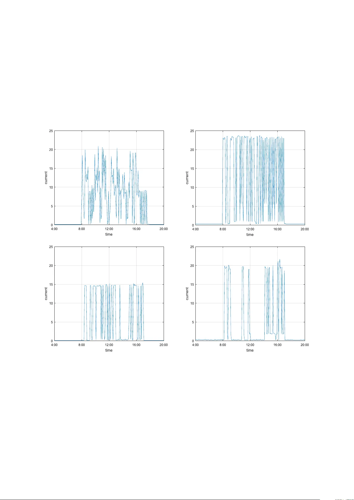
Energy Disaggregation for SMEs using Recurrence Quan tification Analysis Laura Hattam and Danica V uk adino vi´ c Greetham ∗ F ebruary , 2018 Abstract Energy disaggregation determines the energy consumption of individual appliances from the total demand signal, which is recorded using a single monitoring device. There are v aried approaches to this problem, whic h are applied to differen t settings. Here, we fo cus on small and medium en terprises (SMEs) and explore useful applications for energy disaggregation from the persp ectiv e of SMEs. More precisely , w e use recurrence quantification analysis (R QA) of the aggregate and the individual device signals to create a tw o-dimensional map, which is an outlined region in a reduced information space that corresp onds to ‘normal’ energy demand. Then, this map is used to monitor and con trol future energy consumption within the example business so to improv e their energy efficiency practices. In particular, our prop osed method is shown to detect when an appliance ma y b e fault y and if an unexp ected, additional device is in use. 1 In tro duction In recent years, sev eral active energy management solutions ha ve b een developed that are targeted at large manufacturers with integrated systems. Also, a wide range of household micro-systems are b ecoming a v ailable, whic h tak e adv antage of the current smart meter roll-out. In con trast, v ery few meso-lev el systems, i.e. those targeted at small and medium enterprises (SMEs) are presently av ailable. A recent researc h by the UK gov ernment 1 has shown that a very small n um b er of SMEs are actively engaged in energy management, including the use of smart or adv anced meter data. During the last tw ent y y ears, the main consistent barriers are the lack of funds for capital equipmen t and the lac k of in-house expertise to monitor and manage systems. Ho wev er, it is clear that, in principle, SMEs could ac hieve substantial energy cost savings simply through some c hanges in their usage b ehaviour. Resp onding to this gap in the mark et, here we will outline a metho d for monitoring and con trolling energy usage within a small to medium sized business. The energy consumption of an example dry cleaners o ver a six week p eriod is used here to demonstrate the prop osed technique. F rom curren t data collected on site, a disaggregation algorithm is devised so that certain electrical devices and/or device com binations can b e identified from the aggregate energy demand. This allows for the b ehaviour of select devices to be monitored within an example en vironment and as a result, form con trol solutions to impro ve the energy efficiency of its op erations. Since individual device monitoring is exp ensive, energy disaggregation is an extremely useful to ol for energy management as it enables the monitoring of multiple devices with only one smart meter. The main tec hnique adopted here to p erform energy disaggregation is recurrence quan tification analysis (R QA) of a recurrence plot, which was firstly prop osed by Zbilut and W ebb er (1992). More sp ecifically , a recurrence plot is constructed to reveal the repeating patterns within a complex time series that are initially somewhat ∗ Departmen t of Mathematics and Statistics, Universit y of Reading, Whiteknights, Reading, UK 1 https : / / www . gov . uk / government / publications / smart - metering - in - non - domestic - premises - early - research - findings 1 hidden. Then, RQA is p erformed to quantify the recurrent structures illustrated by these plots, where time dep enden t R QA v ariables are computed. The c hosen approach is motiv ated by the findings of F abretti and Auslo os (2005) and Marwan et al. (2013). They demonstrated that by computing R QA v ariables for some time series, significan t even ts and phase transitions could b e detected, such as financial bubbles, financial crashes and transitions in climate systems. In addition, Mosdorf and Gorski (2016) applied R QA to v arious time series that w ere asso ciated with different flow patterns. Consequen tly , certain RQA measurements w ere selec ted that b est captured the b ehaviour of eac h flo w. Next, principal comp onent analysis (PCA) reduced the n umber of comp onen ts do wn to tw o. Lastly , as a function of these tw o comp onents, individual, appro ximate zones were outlined that corresp onded to the different flo w patterns. W e build up on the studies of Mosdorf and Gorski (2016) here by using a similar approac h for the new application of energy disaggregation. Our proposed metho d w orks for lo w er data resolution, and also uses PCA to map selected R QA measuremen ts to t wo comp onen ts. Then, distinct regions within the reduced space are highligh ted to represent differen t usage b ehaviours, whic h allo ws for an in tuitive and easy visualisation of the data in the form of 2-d maps. This is again v ery relev ant to SMEs as it enables the engagement of non-exp ert users, whilst ensuring that the equipment is lo wer in cost and the data storage requirements are minimised. The outline of this pap er is the follo wing: in Section 2 we giv e a short ov erview of relev ant literature on SME energy management, other energy disaggregation metho ds, and direct the reader to RQA metho dology pap ers and its application in v arious fields; then in Section 3 we describe the data used for our case study; in Section 4, the details of our metho d are given, and in Section 5, the visualisation process is describ ed; the metho d results obtained for the case-study data are discussed in Section 6; finally , we conclude in Section 7, where details of future w ork are given. 2 Previous work With increasing in terest in energy efficiency measures, most of the atten tion has naturally b een focused on households and on the largest commercial energy consumers, whic h are on opp osite ends of the sp ectrum in terms of energy consumption (see Sch ulze et al. (2016)). Con versely , enterprises sitting somewhere in b et w een these tw o groups ha ve b een somewhat o verlooked. Due to the heterogeneous nature of SMEs, it is difficult to dev elop a generalised approac h, where the existing literature is split o ver v arying industrial sectors. In addition, trying to cop y the solutions from larger industries does not alwa ys work in the con text of SMEs. F or example, Kannan and Boie (2003) examined a case study on SME’s energy management practices, whic h rev ealed that SMEs are unable to app oin t a dedicated energy manager since the potential energy sa vings do not outw eigh the p osition costs. T rianni and Cagno (2012) inv estigated different barriers to energy efficiency for SMEs and iden tified that the ma jor three are access to capital, lac k or imperfect information on cost-efficien t energy in terven tions and the form of information. They also warned against bundling up together small, medium and large sized enterprises as they usually hav e differen t issues. Blass et al. (2014) studied energy efficiency measures among SMEs in the USA, where top op erations managers are identified as b eing key to enforcing new energy saving measures. F rom all of this, it is safe to assume that the p ersonnel who will b e adopting the new practices is in general a non-exp ert, and therefore, an y metho ds dev elop ed for SMEs need to be accessible and affordable in order to b e considered. Energy disaggregation is an activ e field of researc h due to, amongst other reasons, its relev ance to energy efficiency strategies. Armel et al. (2013) argued that numerous user-b enefits resulted b y making a v ailable the appliance-level energy data, and the com bination of algorithms and smart meters is the most cost- effectiv e/scalable solution to obtaining this data. It was also claimed that disaggregation is often used to pro vide recommendations (e.g. audits or appliance replacemen ts), to detect malfunctions, and to enable new b eha viours. Again, on a commercial level, these are mostly un tapp ed savings in SMEs. Non-in trusive appliance load monitoring (NALM, sometimes NILM or NIALM, see Zoha et al. (2012)) is the disaggregation of a household’s total energy consumption in to individual device consumption, which uses analytical tec hniques only . There is currently a lot of researc h in mac hine learning metho ds for NALM 2 (for an example, refer to T abatabaei et al. (2017)). How ever, these algorithms that disaggregate p ow er loads at low sampling rates of sev eral minutes or half hourly are still not accurate enough, nor practical, as they require substan tial customer input and long training perio ds. Two lo w-rate NALM tec hniques, one com bining k-means clustering and Support V ector Machine, and another requiring a database of appliance signatures created using publicly a v ailable datasets are outlined by Altrabalsi et al. (2016). Due to the heterogeneit y of SMEs, it is exp ected that the creation of a signature database that encompasses all the different appliance scenarios will b e challenging and time consuming, when compared to household appliances that are widely used and mass pro duced. W e are con tributing to this field of researc h by in tro ducing R QA to SME energy disaggregation, whic h to our kno wledge is a no vel application for RQA. W e will show that this metho d do es not require any mac hine learning, it works in low resolutions and the results can be easily visualised. These features allo w us to create an in tuitiv e non-expert in terface for monitoring/con trolling energy usage, whic h will b e esp ecially useful in a SME context. Recurrence is a fundamen tal prop ert y of dynamical systems, and captures the system’s b eha viour in phase space. In order to facilitate visualisation and analysis of recurrences within a time series, Eckmann et al. (1987) in tro duced recurrence plots. Later, the quan tification of recurrence plots and RQA was prop osed in the early 1990s, and has been shown to b e extremely useful for detecting transitions in the system dynamics, as w ell as other relev ant system prop erties. F or the mathematical details of RQA and an o verview of its applications across economy , physiology , neuroscience, earth sciences, astrophysics and engineering, refer to Marw an et al. (2007). 3 Dry Cleaners Data F or six w eeks, energy data was recorded at the dry cleaners, with current readings every five min utes, for the following appliances: 1. Dry er- single phase 2. T able press- three phase 3. Iron- three phase 4. Cleaner- three phase 5. Aggregate- three phase W e c ho ose to fo cus now and for the remainder of the pap er on one phase whic h has all four devices connected. Examples of the daily curren t demands for this phase and the v arious appliances are exhibited in Figure 1. By analysing this data o ver the monitored six w eeks, it is found that the iron and cleaner switc h on and off contin uously throughout the da y , ev ery w orking day . In contrast, the dry er switc hes on ev ery working da y , except sometimes it is off for parts of the day . Lastly , the table press is used every da y , switc hing on and off contin uously throughout the da y , except for nine non-consecutive days when it remains switched off all day . Note that due to the energy information being defined at v arying times, with readings every fiv e min utes i.e. device A and B b egin recordings at, sa y , 00:01 and 00:03 resp ectiv ely , we linearly interpolate the data so that it is then defined every minute. As w ell, the dry cleaners is closed on Sunda ys, and therefore, the data asso ciated with these closure days is omitted. 4 Energy Disaggregation Metho d F or a data set consisting of the curren t profiles for the individual appliances and the aggregate demand, w e apply the following energy disaggregation metho d: 3 Figur e 1: Example daily curr ent demand (Amps) for the devic es: cle aner (top left), ir on (top right), table pr ess (b ottom left), dryer (b ottom right). 4 1. The recurrence plots are constructed for the aggregate signal and the individual device signals. 2. Next, RQA v ariables are computed using a sliding windo w along the recurrence plot diagonal. 3. The R QA measurements found in step 2 are then asso ciated with the particular appliance or appliance com bination when ‘on’ (R QA data corresp onding to a device’s ‘off ’ state is omitted from the analysis). 4. This process is rep eated for a n umber of w eeks so that the range of RQA v alues for each device/device com bination is obtained. 5. N R QA v ariables are chosen that best characterise the v arious appliance states, where N > 2 is some in teger. 6. PCA is next p erformed to reduce this problem from N comp onents to t wo. 7. The R QA information for eac h appliance/appliance com bination is plotted as a function of the tw o comp onen ts determined in step 6. 8. Then, distinct regions are highlighted in this tw o dimensional space to corresp ond to each de- vice/device com bination. F urthermore, the union of these outlined regions creates a map to represent a zone of ‘normal’ energy usage, whic h can b e later used for con trol solutions. The theory asso ciated with this metho d is further detailed in Sections 4.1-4.3. Note that when construct- ing a recurrence plot for the one-dimensional time series Y = ( Y 1 , Y 2 , . . . , Y n ) of length n , often Y is initially embedded in a higher dimensional space (see Kan tz and Schreiber (2003)). How ever, through exp erimen tation with the dry cleaners data, it was concluded that embedding is unnecessary here. 4.1 Recurrence Plots T o create the recurrence plot for the time series Y = ( Y 1 , Y 2 , . . . , Y n ), firstly the distance matrix (DM) is calculated, which is a matrix of p oin ts D M ( i, j ), where i, j = 1 , 2 , . . . , n . The v alue at entry D M ( i, j ) is defined as the distance b etw een Y i and Y j i.e. D M ( i, j ) = | Y i − Y j | , where the matrix aligns v ertically with time step i and horizon tally with time step j . This means that the elements along the diagonal are equal to zero and the matrix is symmetric ab out the diagonal. F rom the DM, the recurrence plot is determined, whic h is a matrix of points R ( i, j ) defined as R ( i, j ) = H (  − D M ( i, j )) , (1) where H ( x ) = ( 0 , if x < 0 , 1 , otherwise . (2) Th us, the entry R ( i, j ) equals one when the distance b etw een Y i and Y j is within the threshold  . When this o ccurs, ( i, j ) is considered recurren t and is lab elled as a recurrence point. No w, since Y i represen ts some curren t level and if R ( i, j ) = 1, then the p oin t Y j is within some neighbouring region of Y i and therefore, the curren t lev el at time step i is similar to the current lev el at time step j . Therefore, using recurrence plots allows us to unco ver an y reoccurring behaviours within our curren t time series. 4.2 Recurrence Quantification Analysis R QA is the tec hnique applied to quan tify the repeating patterns observed within the recurrence plots. The follo wing v ariables are the measures considered here: RE C = 100 × (no. of recurrence p oints within the window) W ( W − 1) , (3) 5 whic h is the p ercen tage of all p oin ts within the square window of size W that are recurren t. D E T = 100 × (no. of recurrence p oints forming diagonal line segmen ts) (no. of recurrence p oints) , (4) whic h is the p ercen tage of the recurrence p oints that form line segments parallel to the matrix diagonal. These structures relate to rep eating or deterministic patterns within the system. E N T = − X P log 2 ( P ) , (5) where P is the probability distribution for the length of the diagonal line segmen ts. E N T is the Shannon en tropy of the distribution of diagonal line segments. This v ariable represen ts complexit y , where small and large E N T signify p erio dic and unpredictable behaviour resp ectiv ely . LAM = 100 × (no. of recurrence p oints forming v ertical line segmen ts) (no. of recurrence p oints) , (6) whic h is the p ercentage of the recurrence p oin ts that form v ertical line segments. These structures represen t stationary b eha viour. T T = av erage length of the v ertical line segmen ts , (7) whic h is the mean length of the vertical line segments. Since our data consists of a set of long time series, eac h series is separated in to a n umber of equally sized subseries referred to as epo chs. Then, the R QA v ariables are calculated at every ep och. As a result, we observ e ho w the R QA measurements v ary as a function of time. This pro cess is ac hiev ed here b y sliding a square window of size W along the diagonal of the recurrence plot, whilst performing R QA at every time incremen t. 4.3 Principal Comp onent Analysis F or information expressed in terms of man y v ariables, PCA calculates an orthogonal basis to describ e this data so that the n um b er of v ariables can b e minimised. This tec hnique is applied here to reduce the n umber of R QA v ariables represen ting each device/device combination. T o b egin, we form a set of n vectors U i of length m , where i = 1 , 2 , . . . , 5 relates to each device t yp e (cleaner, iron, table press, dryer, aggregate), n = 5 is the num b er of device states and m = 5 is the num b er of RQA v ariables considered. The vector U i is defined as U i = mean ( RQA i ) , (8) where RQA i = [ RE C i , D E T i , E N T i , LAM i , T T i ] , (9) whic h is a matrix that corresp onds to the R QA information computed for device i using the metho d of a sliding window, as detailed in Section 4.2. Next, the av erage feature of the set U i is found, which is given b y ψ = 1 n n X i =1 U i , (10) and the cov ariance matrix is obtained using C = 1 n n X i =1 φ i φ T i = AA T , (11) where φ i = U i − ψ and A = [ φ 1 φ 2 · · · φ n ]. 6 Figur e 2: L eft: 2-d map of the R QA information c ompute d fr om 6 we eks of data, which includes the RQA variables: DET, ENT, LAM, TT, REC for the devic es/devic e c ombination: table pr ess (black), cle aner (blue), dryer (gr e en), ir on (r e d), aggr e gate (magenta). Right: The map which c orr esp onds to the ‘normal’ zone of ener gy usage at the dry cle aners. Let us no w refer to the eigenv ectors of C as V j . These v ectors form the orthogonal basis for our information space. If their corresp onding eigen v alues are small, then these eigen vectors are omitted and therefore, the size of the data space is decreased. The remaining eigen vectors next form the matrix E = [ V 1 V 2 · · · V r ], where r is the num b er of eigenv ectors. Now, the R QA data asso ciated with device i , sa y the v ector R QA i,j of length m , can b e pro jected onto the reduced space suc h that w j i = ( RQA i,j − ψ ) T E , (12) whic h is a v ector of length r < m . Here, we ensure that r = 2 so that the R QA device information is pro jected on to a tw o dimensional space with the co ordinates defined by (12). Consequently , a 2-d map can then b e outlined to depict typical energy demand at the dry cleaners. Note that the optimal c hoice for  and W (refer to Sections 4.1-4.2) corresp onds to when the individual device clusters b ecome mostly distinct/separate within this reduced space. Therefore, the selection of the parameters  and W is determined through exp erimentation and visual assessment of the clusters. 5 The 2-D Map By applying the metho d outlined in Section 4, R QA information is computed for the four dry cleaner devices and the aggregate demand, where  = 6 Amps and W = 80 min utes (see Sections 4.1-4.2). This information is then pro jected on to a t wo dimensional space, whic h is illustrated by Figure 2, left. The RQA information clusters corresponding to each device and aggregate demand are highligh ted in this figure, where the table press, cleaner, dryer, iron and aggregate signals corresp ond to the black, blue, green, red and magen ta clusters respectively . Next, the information ‘hot-sp ots’ for eac h device/device com bination are determined using data densit y plots, whic h when combined form the map depicted in Figure 2, righ t. This map signifies ‘normal’ energy consumption at the dry cleaners and is associated with a certain energy budget. It can also b e used to monitor their future demand, where newly recorded aggregate demand is pro jected on to this space. Then, by coun ting the n umber of data p oin ts that pro ject b eyond the map b oundaries, a metric is obtained for assessing how ‘normal’ this aggregate signal is. Moreov er, if a significant p ortion of the data is found to fall outside the map, this can b e used to infer un usual activit y , which could include an additional, unexp ected device switc hing on or a fault y appliance. Refer to Figure 3 for an illustration of this technique, where an example week of aggregate demand (left), is pro jected on to the 2-d space (righ t) 7 Figur e 3: L eft: An example we ek of aggr e gate demand. Right: The signal on the left pr oje cte d onto the 2-d sp ac e (darker c olours c orr esp ond to incr e ase d data density), which fal ls outside the map 248 times. and the num b er of data p oints that fall outside the map is counted (248 p oin ts). Note that this signal mainly sits within the region asso ciated with the combination of all four devices (the magenta cluster in Figure 2, left). This is exp ected since generally at least t wo appliances are alwa ys switc hed on at the dry cleaners. Next, so that the user can b e made a ware of an y unexpected usage behaviour, the installation of an alarm system on site would b e needed such that an alert is giv en when the aggregate signal starts pro jecting outside the map consisten tly . Firstly ho wev er, an appropriate threshold m ust be imp osed corresp onding to when an alarm is triggered. The metho d used here for calculating this threshold is explained in Section 6. 6 Results The map for monitoring energy demand at the dry cleaners has no w b een created (see Figure 2, right). Next, this map and the prop osed alarm system are applied so that the user can main tain a predetermined energy budget, where this set budget relates to daily usage in Section 6.1 and to w eekly usage in Section 6.2. The weekly analysis of the aggregate demand is used here to identify a faulty mac hine. 6.1 A Daily Energy Budget Firstly , to monitor and assess future daily aggregate demand, a threshold needs b e set for the n um b er of times the daily signal must pro ject outside the map to activ ate an alarm. T o compute this, we sim ulate future aggregate demand by randomly selecting daily cleaner, iron, table press and dryer profiles, summing them and then pro jecting this result onto the 2-d space. Next, the n um b er of times this signal pro jects outside the map is coun ted. This is rep eated 100 times so that a probabilit y distribution for the n umber of daily crossings outside our map is obtained, which is display ed in Figure 4, left. The threshold is then c hosen as the upper b ound of this distribution. Here, the alarm threshold of 156 is c hosen (the 90% quan tile), which corresp onds to alerts b eing triggered 10% of the time (approximately 3 alarmed days during a 1 mon th p erio d). Hence, our map representing t ypical energy demand at the dry cleaners and the applied limit of 156 daily crossings, can b e used to monitor and control their daily energy consumption. W e w ant to no w determine if this prop osed method can detect the use of an additional device of compara- ble magnitude. The alert system can then make the dry cleaners aw are that they are p otentially exceeding their predetermined daily energy budget. T o ac hieve this, multiple sim ulations are again p erformed us- 8 Figur e 4: Pr ob ability distributions for the numb er of daily cr ossings outside the map, c ompute d fr om 100 runs using the simulate d daily aggr e gate signal: tabl e pr ess + cleaner + dr y er + ir on (left) and tabl e pr ess + cl eaner + dr y er + ir on 1 + iron 2 (right). Setting the thr eshold to 156 cr ossings outside the map in a day me ans that alerts ar e r e c eive d 10% (left) and 77% (right) of the time. ing the steps previously outlined, except no w a second randomly selected iron profile is also applied i.e. table pr ess + cleaner + dry er + ir on 1 + ir on 2 . As a result, a probability distribution for the n umber of daily crossings is again found, whic h is depicted in Figure 4, righ t. This figure demonstrates that with an alarm threshold of 156, the user will receiv e an alert 77% of the time (approximately 24 alarmed days during a 1 month perio d), which suggests that the addition of another iron in the w orkplace is recognised and sufficient w arning is received b y the user. 6.2 Detecting a F ault y Device Next w e wan t to assess whether our mapping technique can detect a fault y device by sim ulating a cleaner with a defect. This appliance is c hosen as its condition is of most concern at the dry cleaners. Numerous studies, whic h include Thomson and F enger (2001), Luo et al. (2016), Singh and Kumar (2017) and Culbert and Letal (2017), ha ve demonstrated that by analysing the frequency sp ectrum of a machine’s current signal, v arious faults can be recognised due to some change in its frequency information. This approac h is referred to as ‘motor current signature analysis’. Therefore, here we generate a current signal for a fault y cleaner by mo difying its frequency information slightly , whilst main taining a similar amplitude, as w ell as consisten t ‘on’/‘off ’ timings. Also, this signal is initially defined ev ery 5 min utes, and then linearly in terp olated so that it has readings every minute. The result is exhibited in Figure 5, where the frequency sp ectrum of the cleaner current signal and its fault y count erpart are depicted on the left and middle resp ectiv ely . Also, Figure 5, right, p ortra ys an example of the daily current demands for the different cleaner types. T o use our map to no w monitor machine health, a w eekly alarm threshold is instead imp osed. This is b ecause the cleaner is serviced yearly , which is the only appliance that is routinely serviced at the dry cleaners, and therefore, presumably machine faults are not a daily concern here. This means that the w eekly aggregate signal will be pro jected onto our 2-d space, and then if the n umber of pro jections outside the map exceeds the set threshold, the user is alerted. T o determine this w eekly threshold, the same method as previously outlined is applied so that a probabilit y distribution for the num b er of w eekly crossings is calculated from simulated w eekly aggregate signals ( table press + cleaner + dr y er + ir on ). The resulting distribution is depicted in Figure 6, left. F rom this, the alert lev el of 365 crossings is set, whic h corresp onds to 10% (appro ximately 5 alarmed w eeks during a 1 y ear p erio d). Next, swapping the cleaner signal with its fault y coun terpart, m ultiple simulations are again conducted ( tabl e pr ess + f aulty cl eaner + dr y er + ir on ) 9 Figur e 5: L eft and Midd le: The fr e quency sp e ctrum of the cle aner curr ent signal (left) and faulty cle aner (midd le). R ight: Example of the daily curr ent demands for the cle aner (r e d) and faulty cle aner (blue). Figur e 6: Pr ob ability distributions for the numb er of we ekly cr ossings outside the map, c ompute d fr om 100 runs using the simulate d we ekly aggr e gate signal: tabl e pr ess + cleaner + dr y er + ir on (left) and table press + f aulty cleaner + dr y er + ir on (right). Setting the thr eshold to 365 cr ossings outside the map in a we ek me ans that alerts ar e r e c eive d 10% (left) and 80% (right) of the time. and another distribution is computed, whic h is p ortra yed in Figure 6, right. This illustrates that an alert is triggered 80% of the time (approximately 42 alarmed weeks during a 1 year p erio d). Hence, a subtle change in one appliance’s frequency information can b e detected from the aggregate signal using our metho d. Therefore, this suggests that one appliance with an acquired defect can b e identified from the total demand. This finding will p oten tially hav e imp ortant implications for SMEs since, firstly , early detection of a fault y mac hine means that unexp ected shut-do wns are av oided, the need for routine maintenance is decreased and the op erational costs are reduced. Secondly , this work suggests that the health of m ultiple appliances can b e assessed using a single aggregate monitoring device. 7 Conclusion T o conduct energy disaggregation, a dynamical systems approach was adopted, where system prop erties w ere used to differentiate b et ween the v arious time series asso ciated with differen t appliances. More sp ecifically , the case study of a dry cleaners was used here to demonstrate the effectiveness of R QA for SME energy monitoring and control solutions. In particular, a user-friendly map and alert system w as 10 devised. Firstly , a 2-d map was generated that represen ted typical energy usage patterns at the dry cleaners, as well as corresp onding to a set energy budget. Secondly , the alert system ensured that the user w as made a w are when un usual b ehaviour w as detected. Next, t wo example applications of our prop osed metho d w ere given, where the use of an unexp ected device and a faulty mac hine triggered sufficient user w arnings. Note that the machine with a defect w as sim ulated by mo difying the frequency con ten t of its original signal. Hence, subsequent to our technique, the dry cleaners can monitor their energy usage, ensuring that they are alw ays within a predetermined energy budget. Moreo ver, the health of their four main appliances can b e ev aluated with one aggregate monitoring device, where the fault is detected due to a c hange in a device’s frequency information. This dev elopment has the p otential to considerably reduce their op erational costs, the amount of monitoring equipment and the n um b er of routine services. F uture w ork will include acquiring real curren t data from healthy and unhealth y mac hines so to further explore the algorithm capabilities for fault detection and its resolution limits. In addition, an automated online pro cess will b e dev elop ed to define the energy maps and the optimal alarm threshold for v arying user scenarios. Ac knowledgmen t This w ork was carried out with the supp ort of Innov ate UK and EPSRC through the Resp onsive Algo- rithmic Enterprise pro ject (EP/P030718/1). W e thank our pro ject partner AND T ec hnology Researc h ( http : // andtr . com/ ) for providing us with the data and to Dr V alerie Lynch for sharing with us her kno wledge of SME energy efficiency issues. References H. Altrabalsi, V. Stank ovic, J. Liao, and L. Stanko vic. Low-complexit y energy disaggregation using appli- ance load mo delling. AIMS Ener gy , 4(energy-04-00001):1, 2016. K. Carrie Armel, Abha y Gupta, Gireesh Shrimali, and Adrian Alb ert. Is disaggregation the holy grail of energy efficiency? The case of electricity . Ener gy Policy , 52:213–234, 2013. Sp ecial Section: T ransition P athw ays to a Low Carb on Econom y . V. Blass, C.J. Corbett, M.A. Delmas, and S. Muth ulingam. T op management and the adoption of energy efficiency practices: Evidence from small and medium-sized manufacturing firms in the US. Ener gy , 65: 560–571, 2014. I. Culb ert and J. Letal. Signature analysis for online motor diagnostics: Early detection of rotating mac hine problems prior to failure. IEEE Industry Applic ations Magazine , 23(4):76–81, 2017. J.-P . Ec kmann, S. Oliffson Kamphorst, and D. Ruelle. Recurrence plots of dynamical systems. EPL (Eur ophysics L etters) , 4(9):973, 1987. A. F abretti and M. Auslo os. Recurrnce plot and recurrence quan tification analysis techniques for detecting a critical regime. International Journal of Mo dern Physics C , 16(05):671–706, 2005. R. Kannan and W. Boie. Energy managemen t practices in SME case study of a bak ery in German y . Ener gy Conversion and Management , 44(6):945–959, 2003. H. Kantz and T. Sc hreib er. Nonline ar Time Series Analysis . Cambridge Univ ersity Press, Cambridge, UK, 2003. Yin Luo, Shouqi Y uan, Jianping Y uan, and Hui Sun. Induction motor curren t signature for centrifugal pump load. Pr o c e e dings of the Institution of Me chanic al Engine ers, Part C: Journal of Me chanic al Engine ering Scienc e , 230(11):1890–1901, 2016. 11 N. Marwan, M.C. Romano, M. Thiel, and J. Kurths. Recurrence plots for the analysis of complex systems. Physics R ep orts , 438(5):237–329, 2007. N. Marw an, S. Schink el, and Jurgen Kurths. Recurrence plots 25 years later- gaining confidence in dy- namical transitions. EPL (Eur ophysics L etters) , 101(2):20007, 2013. R. Mosdorf and G. Gorski. Identification of tw o-phase flow patterns in minic hannel based on RQA and PCA analysis. International Journal of He at and Mass T r ansfer , 96:64–74, 2016. M. Sch ulze, H. Nehler, M. Ottosson, and P . Thollander. Energy managemen t in industry: A systematic review of previous findings and an in tegrative conceptual framework. Journal of Cle aner Pr o duction , 112:3692–3708, 2016. S. Singh and N. Kumar. Detection of b earing faults in mec hanical systems using stator current monitoring. IEEE T r ansactions on Industrial Informatics , 13(3):1341–1349, 2017. S. M. T abatabaei, S. Dic k, and W. Xu. T ow ard non-intrusiv e load monitoring via m ulti-lab el classification. IEEE T r ansactions on Smart Grid , 8(1):26–40, 2017. W. T. Thomson and M. F enger. Curren t signature analysis to detect induction motor faults. IEEE Industry Applic ations Magazine , 7(4):26–34, 2001. A. T rianni and E. Cagno. Dealing with barriers to energy efficiency and SMEs: Some empirical evidences. Ener gy , 37(1):494–504, 2012. 7th Biennial In ternational W orkshop Adv ances in Energy Studies. J.P . Zbilut and C.L. W ebb er. Em b eddings and delays as derived from quan tification of recurrence plots. Physics L etters A , 171(3):199–203, 1992. A. Zoha, A. Gluhak, M.A. Imran, and S. Ra jasegarar. Non-intrusiv e load monitoring approaches for disaggregated energy sensing: A surv ey . Sensors , 12(12):16838–16866, 2012. 12