Sensor and Sink Placement, Scheduling and Routing Algorithms for Connected Coverage of Wireless Sensor Networks

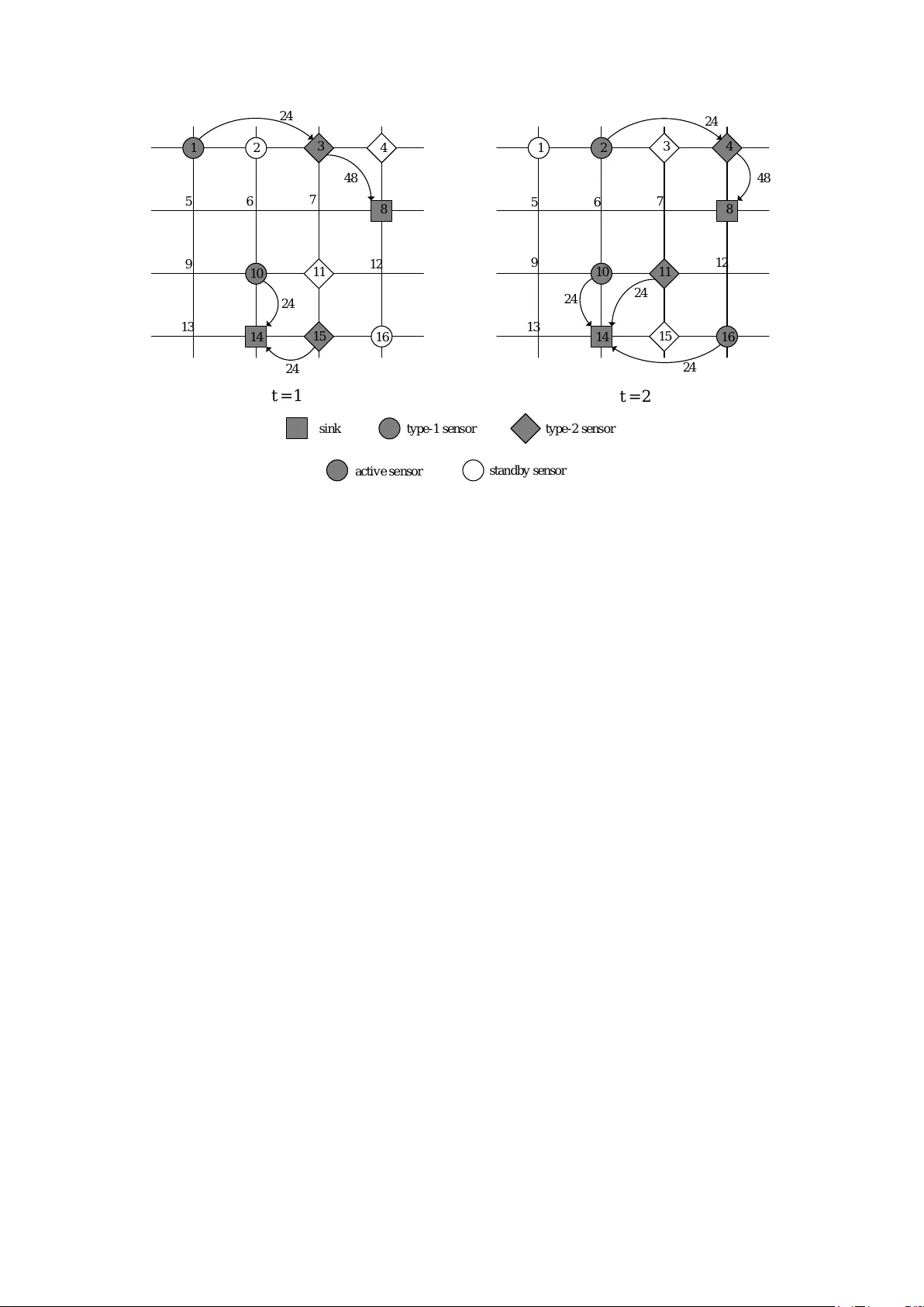
Sensor and Sink Placemen t, Sc heduling and Routing Algorithms for Connected Co v erage of Wireless Sensor Net w orks Ban u Kabakulak ∗ 1 1 Departmen t of Industrial Engineering, Bo˘ gazi¸ ci Universit y , ˙ Istan bul, T urk ey A sensor is a small electronic device whic h has the ability to sense, compute and com- m unicate either with other sensors or directly with a base station (sink). In a wireless sen- sor net work (WSN), the sensors monitor a region and transmit the collected data pac kets through routes to the sinks. In this study , w e prop ose a mixed–integer linear programming (MILP) mo del to maximize the num b er of time p eriods that a WSN carries out the desired tasks with limited energy and budget. Our sink and sensor placement, sc heduling, routing with connected co verage ( S P S RC ) mo del is the first in the literature that com bines the decisions for the lo cations of sinks and sensors, activit y schedules of the deploy ed sensors, and data flow routes from each active sensor to its assigned sink for connected cov erage of the netw ork ov er a finite planning horizon. The problem is NP–hard and difficult to solve ev en for small instances. Assuming that the sink lo cations are kno wn, we develop heuristics whic h construct a feasible solution of the problem by gradually satisfying the constraints. Then, we in tro duce search heuristics to determine the lo cations of the sinks to maximize the net work lifetime. Computational experiments rev eal that our heuristic methods can find near optimal solutions in an acceptable amount of time compared to the commercial solver CPLEX 12.7.0. Keyw ords: Wireless sensor net works, co verage, α − connectivity , activity scheduling, data routing, heuristics. ∗ Corresponding author. T el.: +90 2123596771; fax: +90 2122651800. E-mail addresses: banu.k abakulak@b oun.edu.tr (B. Kabakulak). 1 In tro duction Wireless sensor netw orks (WSNs) are comp osed of a large num b er of wireless devices, called sensor s, equipp ed with communication and computing capabilities to monitor a r eg ion . A homog eneous WSN consists of identical sensors, whereas the communication and computing capabilit y of the sensors are differen t in a heter ogeneous netw ork. WSNs are applied to v arious fields of technology thanks to their easy and cheap deplo yment features. They are used to gather information about human activities in health care, battlefield surv eillance in military , monitor wildlife or p ollution in environmen tal sciences, and so on [30]. A sensor can collect data within its sensing r ange , process data as pack ets and transmit to a base station ( sink ) either directly or through other sensors which are within its c ommunic ation r ange . Sensors consume energy for sensing , r eceiv ing data from other sensors and tr ansmitting data to other sensors or a sink. Energy-a ware op erating is imp ortan t for a sensor since it has limited battery energy . A sensor can carry out sensing and communicating tasks when it is activ e and consumes negligible energy in standby mo de [13]. A sensor is no more a member of the WSN, when its battery energy depletes. The num b er of time p eriods that a WSN op erates as desired is its lif etime and dep ends highly on the limited energy of the sensors. Hence, energy–aw are usage of the sensors helps to prolong the net work lifetime. The key factors that affect the energy consumption can b e listed as follo ws: lo cations of the sensors and sinks in the netw ork, schedule of the active or standby p eriods of the sensors, sink assignmen ts of the sensors and data transmission routes from the sensors to their assigned sinks. Design problems related with WSNs are well studied in the literature. The Cov erage Problem (CP) fo cuses on how well the sensors observ e the region they deploy ed. Eac h no de in the region has a c over age r e quir ement , i.e., least num b er of sensors that should monitor the no de. In order to minimize the energy consumption, CP aims to lo cate smallest num b er of sensors in the region to satisfy the co verage requirements of the no des [28, 33]. The reviews [7, 8] summarize the w orks on CP . A genetic algorithm is prop osed in [21] to cov er each no de with at least one sensor. The greedy algorithm in [4] pro vides cov erage when the sensing ranges of the sensors are adjustable. In [15], the column generation algorithm lo cates the sensors while minimizing the sensing energy consumption of the sensors. In [23], mobile robots are used in coop eration with a WSN to monitor a disaster area. In this study , w e consider differ entiate d CP , where each no de in the netw ork has different cov erage requirement. The active sensors should b e connected to a sink to transmit the sensed data. Cov erage and connec- tivit y are imp ortan t for a WSN, since they are qualit y of service (QoS) measures. There are differen t 2 definitions in the literature for netw ork connectivity . A netw ork can b e considered to b e connected if the active sensors can communicate at least one of the other active sensors [25]. The authors restore the connectivity among the sensors with a heuristic algorithm in the case of a failure of sensors in [14]. Another definition is the existance of a path from each active sensor to a sink in order to transmit the data pack ets [2]. Hence, the lo cations of the sensors are determined to satisfy the co verage require- men ts of the no des and pro vide the connectivity in the Connected Co v erage Problem (CCP). In [9], the authors give energy efficient algorithms for CCP . There are n umerous works in the literature on CCP such as [1, 31, 34]. In our study , we make a broader definition of connectivity and we assume a net work is α − connected in a p erio d if eac h active sensor can comm unicate with α − many activ e sensors and there is a data flo w path to its assigne d sink . Hence, eac h activ e sensor can communicate with its assigned sink either directly or via other active sensors by multi-hop transmission. Moreo ver, one can find alternative paths from the sensors to the sinks in the case of unexp ected failure of a sensor in the net work, since there are at least ( α − 1) active sensors in the communication range of each sensor. One can use the limited energy of the sensors more economically by keeping unnecessary sensors in standb y mo de in a p eriod. That is, the Activity Scheduling Problem (ASP) determines the activ e and standb y p eriods of the sensors in order to extend the netw ork lifetime [17, 20]. The authors schedule the sensors in homogeneous and heterogeneous WSNs in [27]. Heuristic algorithms are developed in [16] to deploy sensors for CP and schedule their activities to maximize the lifetime. In some WSNs, suc h as cognitiv e WSNs, the sensed data pack ets can b e pro cessed by only some of the sink no des. The Sink Assignmen t Problem (SAP) assigns the activ e sensors to an appropriate sink. SAP allows to control the data traffic load on the sinks. This helps to a void congestion, i.e., traffic load exceeds the av ailable capacit y , on the sinks as noted in [10]. The authors formulate the SAP for cognitive WSNs as MILP in [26] and develop a linear relaxation technique for its solution. Sensors also consume energy while transmitting the sensed data to the sinks. Hence, the Data Routing Problem (DRP) finds the minimum energy consuming paths from the active sensors to the sinks [32]. A column generation algorithm is developed in [22] for CCP , ASP , and DRP . An in teger programming form ulation for DRP , when the sensor lo cations are known, is giv en in [29]. The authors introduce cen tralized heuristics to minimize the energy consumption. In the literature, it is sufficient to find a data flow path from a sensor to “a sink.” On the other hand, we extend DRP in this study to design more secure netw orks. That is, w e mak e sink assignment for eac h activ e sensor and construct a data flo w path from a sensor to “its assigned sink.” Such a netw ork design securely collects data, since only the desired sink can receive the data pack ets. The lo cations of the sinks also affect the energy consumption 3 in data routing. The Sink Lo cation Problem (SLP) inv estigates the optimum locations of the sinks that require the least transmission energy . In [18, 24], mobile sinks are considered to collect data from the sensors. The paths of the mobile sensors are also addressed in [12]. The authors develop heuristics to find the lo cations of the sinks at each p eriod. In our study , we assume that sink no des are immobile. In this study , we consider heterogeneous WSNs. W e consider to deploy sensor in the netw ork to satisfy differentiated cov erage requiremen ts of the no des and α − connectivity of the sensors in CCP . W e sc hedule the active and standby p eriods of the sensors for energy–aw are design of the netw ork in ASP . W e assign a sink for each active sensor in a p eriod in SAP . W e detect minimum energy consuming paths from the active sensors to their assigned sinks in DRP . W e find the b est lo cations of the sinks to maximize the net work lifetime in SLP . W e name the netw ork design problem that combines CCP , ASP , SAP , and DRP as the Sensor Placement, Scheduling and Routing with Connectivity ( P S RC ) problem. Additionally , we ha ve the S P S RC problem, which deals with SLP and P S RC simultaneously . S P S RC is difficult to solve exactly for large netw orks since it includes the set cov ering problem, whic h is kno wn to b e NP–complete [5], as a subproblem. W e can list our contribution to the literature as follows: • W e extend the definitions of CCP and DRP by introducing α − connectivity and SAP . • This pap er makes original contributions to the literature by dealing with S P S R C mo del which in tegrates SLP , CCP , ASP , SAP , and DRP . T o the b est of our knowledge, the design issues men tioned are not undertaken within a single mo del in the literature b efore. • W e reduce S P S RC mo del to P S RC by assuming that the sink lo cations are known. W e prop ose Constructiv e Heuristic (CH) and Disjunctive Heuristic (DH) metho ds for the solution of P S R C . • W e generate feasible solutions of S P S R C with our Lo cal Searc h (LS) and T abu Searc h (TS) algorithms, which determine the sink lo cations. • Our solution metho ds can pro vide near optimal feasible solutions of S P S RC in an acceptable amoun t of time. Our algorithms outp erform CPLEX 12.7.0 in terms of solution qualit y and computation time. In the remainder of the paper, we formally define our problem in Section 2 and in tro duce our S P S RC form ulation in Section 3. W e give the details of our heuristic metho ds for the solution of S P S R C in Section 4. W e test the efficiacy of our metho ds via computational exp erimen ts in Section 5. Some concluding remarks and comments on future work app ear in Section 6. 4 2 Problem Definition In this pap er, we consider a heterogeneous WSN with K sensor types giv en with set K = { 1 , ..., K } . W e assume sink is type–0 and set ¯ K = K S { 0 } represents the sensor and sink types. WSN monitors a region defined b y a set of no des, i.e., N = { 1 , ..., N } . W e deploy and activ ate sensors at each time p eriod t ∈ T = { 1 , ..., T } to co ver each no de i ∈ N with at least f i − man y sensors. The cost of placing a sensor ( j , k ), i.e., type- k sensor at lo cation j ∈ N , is given as c j k . W e hav e a total budget of B monetary units. An active sensor ( j, k ) can cov er no des within its sensing ( r s k ) range and generates h j k − man y data pac kets in a p eriod. The co verage co efficien t a j ki is one if sensor ( j, k ) can co ver no de i , and zero otherwise. A type- k sensor can receiv e and transmit data pack ets within its comm unication ( r c k ) range. The communication co efficien t b j ki is one if sensor ( j, k ) can communicate with a sensor or a sink at no de i , and zero otherwise. In order to hav e a robust communication, we require that an active sensor comm unicates with at least α − man y active sensors in a p erio d. A type- k sensor has E k units of energy initially . It consumes e s k units for sensing the netw ork, e r k units for receiving and e c k units for transmitting data pack ets in its active p eriods. A t each p eriod t within netw ork lifetime L , we aim to cov er each no de i and route the data pack ets collected b y the active sensors to their assigned sinks. W e consider T as the planning horizon, which is an upp er b ound on the netw ork lifetime L . W e assume that a sink receives data pack ets but cannot transmit them to other sensors or sinks. That is when there is a sink ( j, 0), w e hav e b j 0 i equal to zero for all i ∈ N . F urthermore, sinks cannot contribute to the cov erage of no des. Hence, for a sink ( j, 0), w e hav e a j 0 i equal to zero for all i ∈ N . W e illustrate a feasible solution of the S P S RC problem with planning horizon T = 2 in Figure 1. In this example, we hav e a 4 × 4 grid netw ork, i.e., N = 16 candidate no des to deploy sinks and sensors. W e hav e tw o different t yp es of sensors ( K = 2) and tw o sinks to collect the data. Co verage requiremen t is one ( f i = 1) for each no de i ∈ N . The sensing range of type–1 sensors is one, and half of the sensing range of type–2 sensors, i.e., 2 r s 1 = r s 2 = 2. The communication range of t yp e–1 sensors is tw o, and half of the communication range of type–2 sensors, i.e., 2 r c 1 = r c 2 = 4. Eac h active sensor communicates with one other active sensor ( α = 1) and generates h j k = 24 data pack ets in a p eriod. In the feasible solution given in Figure 1, the decisions for the netw ork are as follows: • (SLP) Tw o sinks are lo cated at no des 8 and 14 (rectangles), i.e., (8 , 0) and (14 , 0). They are activ e throughout the planning horizon T . 5 1 2 t = 1 t = 2 24 48 24 24 24 24 24 48 sink type - 1 se ns or type - 2 sens or activ e se nsor stan dby sensor 3 4 1 2 3 4 5 6 7 8 5 6 7 8 9 10 11 12 9 10 11 12 13 14 15 16 13 14 15 16 1 2 t = 1 t = 2 48 24 24 24 24 24 48 sink type - 1 se ns or type - 2 sens or activ e se nsor st an db y se ns or 3 4 1 2 3 4 5 6 7 8 5 6 7 8 9 10 11 12 9 10 11 12 13 14 15 16 13 14 15 16 24 24 Figure 1: A sample sensor netw ork op erating for T = 2 • (CCP) W e deplo y four type–1 sensors (circles), i.e., (1 , 1) , (2 , 1) , (10 , 1) and (16 , 1). There are four t yp e–2 sensors (diamonds), which are (3 , 2) , (4 , 2) , (11 , 2) and (15 , 2). • (ASP) In p eriod t = 1, the sensors (1 , 1) , (10 , 1) , (3 , 2) and (15 , 2) are active (black). The sensors (2 , 1) , (16 , 1) , (4 , 2) and (11 , 2) are in standb y mo de (white) at t = 1. In p eriod t = 2, the sensors (2 , 1) , (10 , 1) , (16 , 1) , (4 , 2) , and (11 , 2) are active, whereas (1 , 1) , (3 , 2) and (15 , 2) are in standby mo de. One can observ e that each no de is within the sensing range of at least one active sensor ( f i = 1). F urthermore, there is at least one active sensor ( α = 1) in the communication range of eac h active sensor at each p eriod. • (SAP) The active sensors (1 , 1) and (3 , 2) are assigned to the sink (8 , 0) at t = 1. Besides, (10 , 1) and (15 , 2) are assigned to the sink (14 , 0) in the same p eriod. A t t = 2, the active sensors (2 , 1) and (4 , 2) transmit to the sink (8 , 0), and the sink (14 , 0) collects data from the sensors (10 , 1) , (16 , 1) and (11 , 2). • (DRP) In p eriod t = 1, the sensor (1 , 1) transmits 24 data pack ets to its sink (8 , 0) at 2–hops. The other active sensors can send data to their sinks directly . In p eriod t = 2, the sensor (2 , 1) connects with its sink (8 , 0) via sensor (4 , 2), whereas the other sensors can communicate with 6 their sinks at 1–hop. The solution of DRP provides the paths that connect the sensors to their assigned sinks. 3 Mathematical F orm ulations In this section we introduce a MILP mo del, i.e, S P S R C , that lo cates sinks and sensors, determine activit y schedules of the sensors, assigns a sink for each active sensor and determines the sensor-to-sink data flow routes while maximizing the netw ork lifetime. In the case of kno wn sink lo cations, S P S RC reduces to the sensor placement, scheduling and routing with connected cov erage, i.e., P S RC , mo del. W e ha ve eight decision v ariables in our mathematical mo del. The contin uous v ariable L is the netw ork lifetime that we aim to maximize. The binary decision v ariable n t is one if a perio d t is within the lifetime L , and zero otherwise. The v ariables x j k , z j kt and u ij kt are binary . The v ariable x j k is one if there is a type- k sensor at lo cation j , z j kt is one if the deploy ed sensor ( j, k ) is activ e in p erio d t , and u ij kt is one if the activ e sensor ( j, k ) is assigned to the sink at lo cation i in p eriod t . The amount of flow from sensor ( i, l ) to sensor ( j, k ) in p eriod t is given with the contin uous v ariable y ilj kt . The con tinuous v ariable g ilj t represen ts the incoming flo w to a sink ( j, 0) from sensor ( i, l ) in p eriod t . The binary v ariable w ilj kt is one if there is a p ositiv e flow from sensor ( i, l ) to sensor/sink ( j, k ) in p erio d t , and zero otherwise. W e assume that a sink has sufficiently large battery energy . Hence, a sink is active during the net work lifetime. W e summarize the terminology used in this pap er in T able 1. One can observe that setting all decision v ariables to zero gives a trivial solution with lifetime L = 0. Constrain t (1) eliminates this solution from the solution space. W e hav e n t = 0 when t > L , whic h implies L ≤ t − 1 in constraints (2). 1 ≤ L ≤ T (1) T n t ≥ L + 1 − t, t ∈ T (2) A t each p eriod t within lifetime L , we should cov er a p oin t i ∈ N with at least f i − man y active sensors as given in constraints (3). X ( j,k ) ∈ N K a ij k z j kt ≥ f i n t , i ∈ N , t ∈ T (3) Constrain ts (4) force to deploy a sensor before activ ating it and constraints (5) pro vide not to activ ate a sensor for the p erio ds out of the lifetime L . 7 T able 1: List of symbols Index sets N set of sensor and sink locations K set of sensor types ¯ K set of sensor and sink types T set of p eriods Par ameters a ij k 1 if no de i is within the cov erage range of sensor ( j, k ), 0 otherwise b ilj 1 if a sensor lo cated at no de j is within the com- munication range of sensor ( i, l ), 0 otherwise B total av ailable budget c j k cost of placing a type- k sensor at no de j e c k energy consumption of a type- k sensor for trans- mitting one unit of flow e r k energy consumption of a type- k sensor for receiv- ing one unit of flow e s k energy consumption of a t ype- k sensor for sensing and pro cessing during a p eriod E k initial battery energy of a t yp e- k sensor α minimum num b er of sensors that a sensor can communicate f i cov erage quality requiremen t for no de i h j k num b er of data pac kets generated by sensor ( j, k ) per p eriod N num b er of candidate locations for sensors and sinks K num b er of sensor types r c k communication range of a type- k sensor r s k sensing range of a type- k sensor S num b er of sinks T planning horizon De cision V ariables L lifetime of the WSN n t 1 if p eriod t is within the lifetime L , 0 otherwise x j k 1 if a type- k sensor is placed at no de j , 0 other- wise z j kt 1 if a sensor ( j, k ) is activ e in perio d t , 0 otherwise u ij kt 1 if a sensor ( j, k ) is assigned to a sink located at node i in p eriod t , 0 otherwise y ilj kt amount of data flow from sensor ( i, l ) to sensor ( j, k ) in p eriod t g ilj t amount of data flo w from sensor ( i, l ) to sink ( j, 0) in p eriod t w ilj kt 1 if data flows from sensor ( i, l ) to sensor ( j, k ) in perio d t , 0 otherwise z j kt ≤ x j k , ( j, k ) ∈ N K , t ∈ T (4) z j kt ≤ n t , ( j, k ) ∈ N K , t ∈ T (5) In order to hav e a α − connected netw ork, as given in constrain ts (6), there should b e at least α –many activ e sensors that an active sensor ( i, l ) can communicate at a p eriod t . X ( j,k ) ∈ N K ( j,k ) 6 =( i,l ) b ilj z j kt ≥ αz ilt , ( i, l ) ∈ N K , t ∈ T (6) W e make the unique sink assignments of the active sensors in a p eriod with constrain ts (7)–(9). Constrain ts (7) require a sink ( i, 0) is deploy ed and constraints (8) guarantee that the sensor ( j, k ) is 8 activ e for assigning the sensor ( j, k ) to the sink ( i, 0). Moreo ver, constraints (9) assign one and only one sink for each active sensor ( j, k ) in a p erio d t . u ij kt ≤ x i 0 , i ∈ N , ( j, k ) ∈ N K , t ∈ T (7) u ij kt ≤ z j kt , i ∈ N , ( j, k ) ∈ N K , t ∈ T (8) X i ∈ N u ij kt = z j kt , ( j, k ) ∈ N K , t ∈ T (9) W e av oid flo ws from a sensor ( i, l ) to itself with constraints (10). W e assume that there can be only one active sensor of type- k at a no de in a p eriod, since most of the time an energy efficient optimal solution has such an activity schedule. Hence , the maximum num b er of se n sors that can b e activ e in a p eriod is given by N K . Then, an active sensor ( j, k ) can send the total flo w of ( N K − 1) sensors to a sensor ( i, l ). F rom here, we can b ound the total outflow from an active sensor ( j , k ) b y M 1 = max ( j,k ) ∈ N K { h j k } ( N K − 1). A sensor ( i, l ) can send flow to the sensors that are within its comm unication range as given in constrain ts (11). Constrain ts (12) guaran tee that there is no outflo w from a sensor ( j, k ) in standby mo de. Similarly , total inflow to an activ e sensor ( j, k ) can b e at most M 1 as given in constraints (13). y ililt = 0 , ( i, l ) ∈ N K , t ∈ T (10) y ilj kt ≤ M 1 b ilj , ( i, l ) , ( j, k ) ∈ N K , t ∈ T (11) X ( i,l ) ∈ N K y j kilt ≤ M 1 z j kt , ( j, k ) ∈ N K , t ∈ T (12) X ( i,l ) ∈ N K y ilj kt ≤ M 1 z j kt , ( j, k ) ∈ N K , t ∈ T (13) A sink ( j, 0) can collect the data pack ets of all sensors. A sink ( j, 0) can receive flo ws from the sensors that can communicate with the sink as enforced by constraints (14). Constraints (15) b ound the total inflo w to a sink ( j, 0) by M 2 = max ( j,k ) ∈ N K { h j k } N K . g ilj t ≤ M 2 b ilj , ( i, l ) ∈ N K , j ∈ N , t ∈ T (14) X ( i,l ) ∈ N K g ilj t ≤ M 2 x j 0 , j ∈ N , t ∈ T (15) If a sensor ( j, k ) is active in p eriod t , then it generates h j k units of flow, i.e., data pack ets, to the incoming data flow from the active sensors and sends the total flo w to other active sensors or a sink as outflo w. Constraints (16) ensure the data flow balance for eac h active sensor ( j, k ) in each p eriod t . 9 X ( i,l ) ∈ N K y ilj kt + h j k z j kt = X ( i,l ) ∈ N K y j kilt + X i ∈ N g j kit , ( j, k ) ∈ N K , t ∈ T (16) W e assign a sink for each activ e sensor ( j, k ), which initiates h j k units of data flo w. W e exp ect that the data flo w of each active se nsor reaches to its assigned sink. Constrain ts (17) determine the total inflo w to a sink ( i, 0) as the sum of data flows of the assigned sensors at p eriod t . X ( j,k ) ∈ N K g j kit = X ( j,k ) ∈ N K h j k u ij kt , i ∈ N , t ∈ T (17) An activ e sensor can send its flo w to its assigned sink either directly or through the other active sensors. Then, the sink assignment of a sensor ( i, l ) can b e one of the sink assignments of the sensors that it sends flow. In constrain ts (18), the sink assignment v ariables u v il t of the sensor ( i, l ) is b ounded with the ones of the sensor ( j, k ), i.e., u v j k t , if there is a p ositiv e flow from the sensor ( i, l ) to the sensor ( j, k ). W e assume that a sink ( j, 0) is assigned to itself at all p eriods. In constraints (19), 1 j ( v ) is the indicator function, which takes v alue one if v = j , and zero otherwise. Constraints (19) guarantee that the sink assignment of a sensor ( i, l ) is the sink ( j, 0), if there is a p ositiv e flow among them. u v il t ≤ u v j k t if y ilj kt > 0 , v ∈ N , ( i, l ) , ( j, k ) ∈ N K , t ∈ T (18) u v il t ≤ 1 j ( v ) x j 0 if g ilj t > 0 , v , j ∈ N , ( i, l ) ∈ N K , t ∈ T (19) In a p eriod t , an active sensor consumes energy for sensing and pro cessing the data collected from the region, for receiving data from the other active sensors and transmitting the data to the other active sensors or a sink. T otal consumed energy of a sensor ( j, k ) during its active p erio ds is limited by the initial battery energy E k , which is mo deled with the energy constraints (20). X t ∈ T   e s k z j kt + e r k X ( i,l ) ∈ N K y ilj kt + e c k X ( i,l ) ∈ N K y j kilt + e c k X i ∈ N g j kit   ≤ E k , ( j, k ) ∈ N K (20) Constrain ts (21) force that the total deplo yment cost of sensors and sinks do es not exceed the total a v ailable budget. X ( j,k ) ∈ N ¯ K c j k x j k ≤ B (21) Constrain ts (22) limit the num b er of sinks in the netw ork with S . 10 X i ∈ N x i 0 = S (22) Finally , constraints (23) - (28) are the binary and nonnegativity restrictions on the decision v ariables. n t ∈ { 0 , 1 } , t ∈ T (23) x j k ∈ { 0 , 1 } , ( j, k ) ∈ N ¯ K (24) z j kt ∈ { 0 , 1 } , ( j, k ) ∈ N K , t ∈ T (25) u ij kt ∈ { 0 , 1 } , i ∈ N , ( j, k ) ∈ N K , t ∈ T (26) y ilj kt ≥ 0 , ( i, l ) , ( j, k ) ∈ N K , t ∈ T (27) g ilj t ≥ 0 , ( i, l ) ∈ N K , j ∈ N , t ∈ T (28) W e formulate the sink and sensor placement, scheduling, routing while providing connected cov erage ( S P S RC ) as mixed–integer linear programming problem sub ject to the constraints (1) – (28). W e aim to maximize the netw ork lifetime (29) under limited energy and budget resources. max L (29) One can observe that constraints (18) and (19) are not linear. W e introduce binary v ariables w ilj kt , whic h is one if there is a p ositiv e flow from a sensor ( i, l ) to a sensor/sink ( j, k ) in p eriod t , and zero otherwise. Then, we linearize constraints (18) and (19) as follows: y ilj kt ≤ M 1 w ilj kt , ( i, l ) , ( j, k ) ∈ N K , t ∈ T (30) g ilj t ≤ M 2 w ilj 0 t , ( i, l ) ∈ N K , j ∈ N , t ∈ T (31) u v il t − u v j k t ≤ 1 − w ilj kt , v ∈ N , ( i, l ) , ( j, k ) ∈ N K , t ∈ T (32) u v il t − 1 j ( v ) x j 0 ≤ 1 − w ilj 0 t , v , j ∈ N , ( i, l ) ∈ N K , t ∈ T (33) W e ha ve battery energy limitations of the sensors as constraints (20). This means, there can b e alternativ e optimum solutions of S P S R C mo del whic h consume less energy if we can a void unnecessary flo w lo ops. In constraints (6), we know that an active sensor can communicate with at least α − many activ e sensors. F rom here, we can sav e energy in the net work if we limit the num b er of outflow paths from a sensor ( i, l ) b y α as in constraints (34). 11 X ( j,k ) ∈ N K w ilj kt ≤ α, ( i, l ) ∈ N K , t ∈ T (34) S P S RC combines multiple decisions related with a netw ork in one mo del. S P S RC is an NP–complete problem [5, 19]. Hence, we propose heuristic approaches to generate a near optimal solution of S P S R C in acceptable amount of time. W e first consider that we are given the lo cations of S sinks, i.e., x i 0 v alues are known. W e name this problem as P S RC . W e generate feasible solutions via our constructive heuristic (CH) and disjunctive heuristic (DH) approaches for P S RC . Then, w e find feasible solutions of S P S R C with our lo cal search (LS) and tabu search (TS) metho ds, which determine the lo cations of the sinks. W e explain the details of these algorithms in the next section. 4 Solution Metho ds W e introduce CH (see Section 4.1.1) and DH (see Section 4.1.2) algorithms to generate feasible solutions of P S RC . W e can construct a feasible solution of P S R C with CH or DH either from scratch (all − 0 solution), or improv e a given feasible solution, or repair an infeasible solution. These heuristics are em b edded in to our sink lo cation search algorithms, i.e., LS (see Section 4.2.1) and TS (see Section 4.2.2), explained in Section 4.2 to maximize the netw ork lifetime L . 4.1 F easible Solution Generation Algorithms for P S R C 4.1.1 Constructive Heuristic In Algorithm 1, we explain the main steps of CH. In the first step of CH, w e obtain a feasible solution of P S RC with resp ect to the co verage (3) and budget (21) constraints with Algorithm 2. Then, we satisfy the connectivit y (6) and sink assignment (7) - (9) constraints by assigning sinks to the activ e sensors using Algorithm 3. W e determine the amount of flows y and g from the active sensors to their assigned sinks by solving Routing Problem ( RP ( t )) at each p erio d t . 12 Algorithm 1. (Constructive Heuristic) Input: An instanc e of P S RC , a ve ctor ( L, n , x , z , u , y , g , w ) 0. Set L = T . 1. Apply Algorithm 2 to obtain a feasible solution subje ct to cover age (3) and budget (21) c onstr aints. 2. If L = 0 , Then Stop. 3. Else F or Each t ≤ L 4. Apply Algorithm 3 to gener ate a fe asible solution subje ct to c onnectivity (6) and sink assignment (7) - (9) constr aints in perio d t . 5. End F or Each 6. End If 7. If L = 0 , Then Stop. 8. Else F or Each t ≤ L , solve RP ( t ) to determine the data flows y and g . 9. End If Output: A fe asible solution of P S RC with lifetime L . In order to satisfy the constraints (3) and (21), w e implemen t Algorithm 2. W e estimate the maximum p ossible outflow from an active sensor ( j, k ) in p eriod t as ζ t =   X ( j,k ) ∈ N K z j kt    max ( j,k ) ∈ N K h j k  , t ∈ T . (35) A t the b eginning of each perio d t , we chec k whether an active sensor ( j, k ) ( z j kt = 1) has sufficien t battery energy for sensing and communicating tasks or not. A t p eriod t = 1, we hav e E rem j kt = E k . A sensor ( j, k ) can be active in p eriod t if the remaining battery energy satisfies E rem j kt ≥ ( e s k + ζ t ( e r k + e c k )), w e set z j kt = 0 otherwise (Step 3). W e up date E rem j kt for each p erio d t using Equation (36). E rem j k,t +1 = E rem j kt − z j kt ( e s k + ζ t ( e r k + e c k )) , ( j, k ) ∈ N K . (36) W e chec k whether each no de i in the region is cov ered by f i − man y activ e sensors or not in each p eriod t . If eac h no de is cov ered within the budget in a p eriod t , then we mov e to the next p eriod. If budget constraint is not held, we consider to remov e some of the deploy ed sensors without harming the co verage constrain ts at Step 7. F or this purp ose, we delete sensors, i.e., set x j k = 0, that are in standby mo de until the current p eriod since they do not contribute to the cov erage of the no des in an y of the p eriods. Deleting sensor ( j, k ) improv es remaining budget by c j k monetary units. W e contin ue with the pro cess while the remaining budget is negative or w e cannot find a sensor to delete. After this pro cedure, it is p ossible that we could not provide budget feasibility . In this case, one can consider to delete active s ensors whose remov al will not harm the co verage of the no des. This strategy is used only when w e are in the first p eriod, i.e., t = 1, for the sake of simplicit y of the heuristic. If budget still cannot b e provided then we set L = t − 1 and stop the algorithm (Step 8). On the other 13 hand, if there is an undercov ered no de in the region, then w e first try to ensure cov erage in the netw ork b y activ ating the existing sensors. Observe that activ ating a standby sensor do es not demand budget usage. Algorithm 2. (Satisfying Cover age (3) and Budget (21) Constr aints) Input: An instanc e of P S RC , a p artial (in)fe asible solution ( L, n , x , z ) 0. Set t = 1 . 1. F or Each t ≤ L 2. F or Each active sensor ( j, k ) in perio d t ( z j kt = 1 ), c alculate E rem j kt 3. If E rem j kt is not sufficient, Then z j kt = 0 . 4. End F or Each 5. If every no de is c over e d, Then 6. If budget is satisfie d, Then t ← t + 1 . 7. Else or der standby sensors in [0 , t ] in nonincre asing c ost and r emove them until budget is satisfie d. 8. If budget is violate d, Then n t = 0 , L = t − 1 and Stop. 9. Else While ther e is C E P j k > 0 with sufficient E rem j kt for some sensor ( j, k ) activate ( z j kt = 1 ) the standby sensor ( j, k ) with the highest C E P j k . 10. End While 11. While ther e is a sensor ( j, k ) with the highest C C R j k > 0 12. If budget is not enough for the sensor ( j, k ) , Then or der standby sensors in [0 , t ] in nonincr e asing c ost and r emove them until enough budget is obtaine d. 13. If budget is enough, 14. Then deploy ( x j k = 1 ) and activate ( z j kt = 1 ) the sensor ( j, k ) with the highest C C R j k . 15. Else n t = 0 , L = t − 1 and Stop. 16. End If 17. End While 18. End If 19. End F or Each Output: A solution satisfying the c onstr aints (3) and (21) with lifetime L . W e choose the standb y sensor to activ ate in a gereedy w ay by calculating the c over age ener gy pr o duct , i.e., C E P j k , for each sensor ( j, k ) in a p eriod t . Let ( n , x , z ) be the p ossibly infeasible partial initial solution giv en as input to Algorithm 2. In a p eriod t , w e calculate the amoun t of violation in constrain ts (3) for each no de i with the undercov erage U i v alues as given in Equation (37). U i = max      f i n t − X ( j,k ) ∈ N K a ij k z j kt   , 0    , i ∈ N (37) F or a standb y sensor, it will b e a reason of choice if it can cov er as man y nodes as p ossible that ha ve p ositiv e U i . In addition, as the sensor has more remaining energy in its battery , the need for the deplo yment of new sensors will b e less in the future, since we can activ ate the sensor in these p eriods also. Therefore, we can define C E P j k for a standby sensor ( j, k ) in a p eriod t as 14 C E P j k = P i ∈ N : U i > 0 a ij k ! x j k E rem j kt c j k , ( j, k ) ∈ N K (38) where E rem j kt represen ts the remaining energy of a sensor ( j, k ) in p eriod t . Then, we activ ate the standby sensors starting from the one with the highest p ositiv e C E P j k v alue and contin ue until we provi de co verage constrain ts or we do not hav e standby sensors with p ositiv e C E P j k v alue (Step 9). If we could not satisfy constraints (3), then we calculate a c over age c ost r atio , i.e., C C R j k , for each sensor ( j, k ) as C C R j k = P i ∈ N : U i > 0 a ij k ! (1 − x j k ) E k c j k , ( j, k ) ∈ N K (39) where E k represen ts the initial battery energy of a type- k sensor. W e deploy ( x j k = 1) and activ ate ( z j kt = 1) a new sensor ( j, k ) in perio d t with the highest C C R j k v alue (Step 14). In the case remaining budget is not enough to deploy the selected sensor, we try to generate sufficient budget by deleting standb y sensors that are not used un til the current p eriod (Step 12). If cov erage is not provided within the budget, then we set L = t − 1 and stop the algorithm. The computational complexity of Algorithm 2 is giv en as O ( τ 1 N 3 K T + τ 1 N 2 K T 2 ) where τ 1 = max i ∈ N ( P ( j,k ) ∈ N K a ij k ) is the maxim um num b er of sensors that can cov er a no de. 15 Algorithm 3. (Satisfying Conne ctivity (6) and Sink Assignment (7) - (9) Constr aints) Input: An instanc e of P S RC , p eriod t , a p artial (in)feasible solution ( L, n t , x t , z t , u t ) 0. Set u t = 0 . L et L b e a list of sensors and sinks. A dd S − many sinks to L and lab el them. 1. While L is not empty 2. If the first element of L is a sink (say ( j, 0) ), Then add unlab ele d active sensors ( i, l ) that c ommunic ate with the sink ( j, 0) , i.e., b ilj = 1 , to list L . Set u j ilt = 1 . R emove sink ( j, 0) from list L . 3. Else /* the first element of L is a sensor (say ( j, k ) ) */ add unlab ele d active sensors ( i, l ) that c ommunic ate with the active sensor ( j, k ) , i.e., b ilj = 1 , to list L . Set u vilt ← u vj kt for al l v ∈ N . R emove sensor ( j, k ) from list L . 4. End If 5. End While 6. If c onne ctivity is not satisfie d, Then 7. While ther e is C oE P j k > 0 with sufficient E rem j kt for some sensor ( j, k ) activate ( z j kt = 1 ) the standby sensor ( j, k ) with the highest C oE P j k . 8. End While 9. While ther e is a sensor ( j, k ) with the highest C oC R j k > 0 10. If budget is not enough for the sensor ( j, k ) , Then or der standby sensors in [0 , t ] in nonincr e asing c ost and r emove them until enough budget is obtaine d. 11. If budget is enough, 12. Then deploy ( x j k = 1 ) and activate ( z j kt = 1 ) the sensor ( j, k ) with the highest C oC R j k . Pick a sensor ( i, l ) with b j ki = 1 , and set u vj kt ← u vilt for al l v ∈ N . 13. Else n t = 0 , L = t − 1 and Stop. 14. End If 15. End While 16. End If Output: A solution satisfying the c onstr aints (6) and (7) - (9) for p erio d t . W e satisfy the connectivit y (6) and the sink assignment (7) - (9) constraints in a p eriod t with Algorithm 3. W e carry out a breadth–first–searc h starting from S − many sinks to detect the active sensors that can communicate with one of the sinks (Step 2) or another activ e sensor that has a sink assignmen t (Step 3). If each active sensor cannot communicate with at least α − many active sensors as constrain ts (6) require, w e first consider to activ ate some of the standby sensors ( j , k ), since this is cost free. Among the standb y sensors ( j, k ) having E rem j kt ≥ ( e s k + ζ t ( e r k + e c k )) remaining battery energy , we activ ate the one which has the highest p ositiv e c ommunic ation ener gy pr o duct , i.e., C oE P j k (Step 7). Let ( x t , z t ) b e the partial initial solution obtained with Algorithm 2 in p erio d t . Then, we calculate the underconnectivity U C il of the active sensors ( i, l ) with Equation (40). U C il = max            αz ilt − X ( j,k ) ∈ N K ( j,k ) 6 =( i,l ) b ilj z j kt     , 0        , ( i, l ) ∈ N K (40) In order to pro vide connectivit y , w e prefer to activ ate the cheapest standb y sensor that has the highest 16 remaining battery energy and can communicate with most of the underconnected sensors. Hence, we define C oE P j k for a standby sensor ( j, k ) in p eriod t as C oE P j k =    P ( i,l ) ∈ N K U C il > 0 b j ki    x j k E rem j kt c j k , ( j, k ) ∈ N K . (41) If connectivity is not held in Step 12, we consider to deploy ( x j k = 1) and activ ate ( z j kt = 1) the sensor ( j, k ) with the highest p ositiv e c ommunic ation c ost r atio , i.e., C oC R j k giv en as C oC R j k =    P ( i,l ) ∈ N K U C il > 0 b j ki    (1 − x j k ) E k c j k , ( j, k ) ∈ N K (42) where E k represen ts the initial battery energy of a type- k sensor. W e contin ue with the sensor deplo yment as we can find a sensor that has p ositiv e C oC R j k v alue. In the insufficien t budget case, w e remov e the sensors that are in standby mo de upto p eriod t . If w e cannot generate the required budget, we up date the netw ork lifetime as L = t − 1 and stop the algorithm. In the last step of CH (Step 8 of Algorithm 1), we solve RP ( t ) for each p eriod t within the lifetime L to find the minimum energy consuming sensor–to–sink data flow paths. In RP ( t ), y j kil and g j ki are con tinuous v ariables representing the data flows in p eriod t from sensor ( j, k ) to sensor ( i, l ) and from sensor ( j, k ) to sink ( i, 0), resp ectiv ely . W e hav e a partial solution ( ¯ L, ¯ n , ¯ x , ¯ z , ¯ u ) obtained by applying Algorithms 2 and 3. W e initialize the remaining energy of a sensor ( j, k ) in p eriod t = 1 as E rem j k 1 = E k . Let ε t j k b e the v alue of ε j k v ariable in RP ( t ), i.e., energy consumption of the sensor ( j, k ) in p eriod t . Then, we up date the battery energy E rem j k,t +1 at the b eginning of the p eriod t + 1 as E rem j k,t +1 = E rem j kt − ε t j k , ( j, k ) ∈ N K . (43) Observ e that we can find a feasible solution of RP ( t ) for each p erio d t , since we activ ate the sensors that ha ve sufficient energy for transmitting maxim um possible flo w ζ t in Algorithms 2 and 3. W e rewrite the constrain ts (20), (16), (17), (11) – (13), (14), (15), (10) as the constrain ts (44b), (44d), (44e), (44f) – (44h), (44j), (44k), (44m), resp ectiv ely , with y j kil and g j ki v ariables and given ( ¯ x , ¯ z , ¯ u ) v alues in RP ( t ). Constrain ts (44c) b ound the energy consumption with E rem j kt whic h is calculated with the Equations (43). Observe that w v ariables are not required in RP ( t ), since w e can represent the constraints (30) – (33) with the constraints (44i) and (44l). F urthermore, we do not need constraints (34), since R P ( t ) a voids unnecessary flo ws by minimizing the energy consumption. R P ( t ) can b e solved in p olynomial 17 time, since it is a linear programming form ulation [11]. RP( t ) : min X ( j,k ) ∈ N K ε j k (44a) s.t.: ε j k = e s k ¯ z j kt + e r k X ( i,l ) ∈ N K y ilj k + e c k X ( i,l ) ∈ N K y j kil + e c k X i ∈ N g j ki , ( j, k ) ∈ N K (44b) ε j k ≤ E rem j kt , ( j, k ) ∈ N K (44c) X ( i,l ) ∈ N K y ilj k + h j k ¯ z j kt = X ( i,l ) ∈ N K y j kil + X i ∈ N g j ki , ( j, k ) ∈ N K (44d) X ( j,k ) ∈ N K g j ki = X ( j,k ) ∈ N K h j k ¯ u ij kt , i ∈ N (44e) y ilj k ≤ M 1 b ilj , ( i, l ) , ( j, k ) ∈ N K (44f ) X ( i,l ) ∈ N K y j kil ≤ M 1 ¯ z j kt , ( j, k ) ∈ N K (44g) X ( i,l ) ∈ N K y ilj k ≤ M 1 ¯ z j kt , ( j, k ) ∈ N K (44h) y ilj k ≤ M 1   1 − X v ∈ N | ¯ u vilt − ¯ u vj kt | 2   , ( i, l ) , ( j, k ) ∈ N K (44i) g ilj ≤ M 2 b ilj , ( i, l ) ∈ N K , j ∈ N (44j) X ( i,l ) ∈ N K g ilj ≤ M 2 ¯ x j 0 , j ∈ N (44k) g ilj ≤ M 2   1 − X v ∈ N | ¯ u vilt − 1 j ( v ) ¯ x j 0 | 2   , ( i, l ) ∈ N K , j ∈ N (44l) y ilil = 0 , ( i, l ) ∈ N K (44m) y ilj k ≥ 0 , ( i, l ) , ( j, k ) ∈ N K (44n) g ilj ≥ 0 , ( i, l ) ∈ N K , j ∈ N (44o) ε j k ≥ 0 , ( j, k ) ∈ N K . (44p) CH metho d provides feasibilit y with resp ect to co verage (3) and budget (21) constrain ts for all perio ds in the planning horizon T (Step 1 of Algorithm 1). Then, we assign a sink to each of the activ e sensors while satisfying connectivity (6) constraints for all p eriods (Step 4 of Algorithm 1). Lastly , w e find the minimum energy consuming paths from sensors to their assigned sinks for all p eriods (Step 8 of Algorithm 1). CH consumes most of the budget to cov er the netw ork as more p eriods as p ossible in Step 1. This strategy decreases the c hance of providing connectivity b y deploying new se n sors in Step 4, whic h adversely affects the lifetime L . F rom this observ ation, w e prop ose DH metho d (see Section 4.1.2), which considers feasibilit y with resp ect to co verage (3), budget (21), connectivity (6), sink assignment (7) - (9) constraints and determination of data routes for each p eriod indep enden tly . 4.1.2 Disjunctive Heuristic W e summarize our DH metho d in Algorithm 4. W e first set the active sensors, which do not hav e sufficien t battery energy E rem j kt in a perio d t , to standby mo de (Steps 1 - 4). W e treat each p eriod 18 individually , and satisfy constraints in the order of cov erage (3), budget (21), connectivity (6), sink assignmen t (7) - (9). W e remov e standby sensors upto the current p eriod when the budget is not enough to deploy new sensors for cov erage and connectivity (Steps 11 and 18). Algorithm 4. (Disjunctive Heuristic) Input: An instanc e of P S RC , a ve ctor ( L, n , x , z , u , y , g , w ) 0. Set t = 1 , L = T . 1. F or Each t ≤ L 2. F or Each active sensor ( j, k ) in perio d t ( z j kt = 1 ), c alculate E rem j kt 3. If E rem j kt is not sufficient, Then z j kt = 0 . 4. End F or Each 5. F or Each t ≤ L 6. If every no de is c over e d, Then 7. If budget is satisfie d, Then 8. If Algorithm 3 gener ates a fe asible solution subje ct to c onstr aints (6) and (7) - (9) in p erio d t , Then Apply Algorithm 5 to de activate ( z j kt = 0 ) the sensors without violating constr aints (3), (6) and (7) - (9). Solve RP ( t ) to determine the data flows y and g . t ← t + 1 9. Else Stop. 10. End If 11. Else or der standby sensors in [0 , t ] in nonincre asing c ost and r emove them until budget is satisfie d. 12. If budget is violate d, Then n t = 0 , L = t − 1 and Stop. 13. Else apply Steps 8 - 10. 14. End If 15. Else While ther e is C E P j k > 0 with sufficient E rem j kt for some sensor ( j, k ) activate ( z j kt = 1 ) the standby sensor ( j, k ) with the highest C E P j k . 16. End While 17. While ther e is a sensor ( j, k ) with the highest C C R j k > 0 18. If budget is not enough for the sensor ( j, k ) , Then or der standby sensors in [0 , t ] in nonincr e asing c ost and r emove them until enough budget is obtaine d. 19. If budget is enough, 20. Then deploy ( x j k = 1 ) and activate ( z j kt = 1 ) the sensor ( j, k ) with the highest C C R j k . 21. Else n t = 0 , L = t − 1 and Stop. 22. End If 23. End While 24. Apply Steps 8 - 10. 25. End If 26. End F or Each Output: A fe asible solution of P S RC with lifetime L . F urthermore, we sa ve energy with Algorithm 5 by setting the active sensors, which will not harm co verage and connectivity restrictions, to standby mo de (Step 8). W e start deactiv ation from the most exp ensiv e active sensor, since w e can generate more budget if w e consider to remov e standby sensors for cov erage or connectivity in some p eriod. R P ( t ) finds the minim um energy consuming paths for the activ e sensors to their assigned sinks in p eriod t (Step 8). W e mov e to the next p eriod if w e satisfy the 19 constrain ts for the current p eriod. This budget and battery energy utilization strategy improv es the lifetime L compared to CH as we rep ort in Section 5. Algorithm 5. (De activating Unne cessary Sensors) Input: An instanc e of P S RC , p eriod t , a p artial feasible solution ( L, n t , x t , z t , u t ) 0. Let isActiv e = f alse . L et L b e the nonincr e asing c ost order of the active sensors ( j, k ) in p eriod t ( z j kt = 1 ). 1. F or Each active sensor ( j, k ) ∈ L 2. isActiv e = f alse . 3. F or Each no de i with a ij k = 1 4. If c onstr aints (3) ar e violate d for no de i , Then isActiv e = tr ue . 5. End F or Each 6. If isActiv e = f al se , Then 7. F or Each active sensor ( i, l ) with b j ki = 1 8. If c onstr aints (6) ar e violate d for sensor ( i, l ) , Then isActiv e = tr ue . 9. End F or Each 10. End If 11. If isActiv e = f alse , Then 12. De activate sensor ( j, k ) in p eriod t ( z j kt = 0 ). 13. F or Each active sensor ( i, l ) with b j ki = 1 , set u vilt = null for al l v ∈ N . 14. F or Each active sensor ( i, l ) without sink assignment 15. Pick one of the active sensors ( i 0 , l 0 ) with b ili 0 = 1 and set u vilt ← u vi 0 l 0 t for al l v ∈ N . 16. End F or Each 17. End If 18. End F or Each Output: Unnec essary active sensors ar e in standby mo de in p eriod t . The computational complexity of Algorithm 5 is giv en as O ( N 4 K 3 ). 4.2 Sink Searc h Algorithms for S P S RC In this section, we describ e our search heuristics, i.e., LS and TS, to satisfy constraint (22) while maximizing the net work lifetime L . These algorithms estimate the lifetime L with a heuristic for P S RC (see Section 4.1) while se ar ching the lo cations of S − many sinks. 4.2.1 Lo cal Searc h Heuristic In LS heuristic, giv en in Algorithm 6, we explore N candidate lo cations to deploy S sinks. W e assume that x 0 = ( x 10 , x 20 , ..., x N 0 ) with x j 0 ∈ { 0 , 1 } is the binary v ector of sink locations. W e sort N candidate lo cations in nondecreasing sink deplo y cost c j 0 order. Initially , w e lo cate S sinks to the cheapest no des. W e implement a P S R C heuristic (CH or DH) to obtain an initial netw ork lifetime L with the remaining budget ( B − P j ∈ N c j 0 x j 0 ) (Step 0). A t each iteration iter , we randomly change the lo cations of s ≤ S sinks. W e pick a lo cation j with probabilit y p ( j ), which is in versely prop ortional to the sink cost c j 0 as given in Equation (45). W e 20 can hav e more remaining budget for the P S R C problem by economically lo cating the sinks with this strategy . p ( j ) = P i 6 = j i ∈ N c i 0 ( N − 1) P i ∈ N c i 0 , j ∈ N . (45) Giv en the lo cations x 0 of S − sinks, there are N S s =  N − S s  S s  differen t alternatives to relo cate s − sinks. In LS, we scan P s p ercen tage of the neighborho od N S s to determine an improving solution (Step 3). Once we relo cate the sinks, we compute the netw ork lifetime ¯ L with the remaining budget through a P S RC heuristic (Step 4). W e contin ue with the search until we complete iter Lim − man y iterations or we cannot up date the current lifetime L for nI mpr − man y consecutive iterations. Algorithm 6. (L oc al Se ar ch) Input: # of c andidate lo cations N , # of sinks S , iter Lim , nI mpr 0. Set iter = 0 and noI mpr = 0 . L et x 0 b e the ve ctor of sink loc ations. L oc ate S sinks to the cheap est no des. L et L b e the lifetime found by a P S RC heuristic (CH or DH). 1. While iter < iter Lim and noI mpr < nI mpr 2. F or Each s ≤ S 3. F or N S s P s − many trials 4. R andomly change lo c ations of s − sinks. L et ¯ L b e the lifetime found by a P S RC heuristic. 5. If ¯ L > L , Then L ← ¯ L , up date x 0 . 6. End F or 7. End F or Each 8. If L is impr ove d, Then noI mpr = 0 , Else noI mpr ← noI mpr + 1 . 9. iter ← iter + 1 10. End While Output: A fe asible solution of S P S RC with lifetime L . 4.2.2 T abu Searc h Heuristic TS, given in Algorithm 7, aims to visit as distict parts of the solution space as p ossible by forbidding to revisit the recent tabuT enur e − man y solutions from the solution space of sink lo cations [6]. Similar to LS, we lo cate S sinks to the cheapest no des initially . W e swap s − sinks ( s ≤ S ) randomly using the probabilit y density function in Equation (45) to mov e another solution (Steps 2 - 6). W e implement a P S RC heuristic (CH or DH) to determine the netw ork lifetime ¯ L with the cur- ren t sink lo cations (Step 4). In Step 5, we add improving solutions to tabuList , whic h stores recen t tabuT enur e − man y solutions. That is as w e add a new solution to tabuList , we remov e the oldest solu- tion from tabuList . The algorithm stops after iter Lim − man y iterations or nI mpr − man y consecutive nonimpro ving iterations. 21 Algorithm 7. (T abu Se ar ch) Input: # of c andidate lo cations N , # of sinks S , iter Lim , nI mpr , tabuT enur e 0. Set t = 0 , noI mpr = 0 and tabuList = ∅ . L et x 0 b e the ve ctor of sink loc ations. L oc ate S sinks to the cheap est no des. A dd x 0 to tabuList . L et L b e the lifetime found by a P S RC heuristic (CH or DH). 1. While t < iter Lim and noI mpr < nI mpr 2. F or Each s ≤ S 3. F or N S s P s − many trials 4. R andomly change lo c ations of s − sinks to obtain a nontabu ve ctor. L et ¯ L b e the lifetime found by a P S RC heuristic. 5. If ¯ L > L , Then L ← ¯ L , up date x 0 and add to tabuList . 6. End F or 7. End F or Each 8. If L is impr ove d, Then noI mpr = 0 , Else noI mpr ← noI mpr + 1 . 9. t ← t + 1 10. End While Output: A fe asible solution of S P S RC with lifetime L . 5 Computational Results The computations ha ve b een carried out on a computer with 2.0 GHz In tel Xeon E5-2620 pro cessor and 46 GB of RAM working under Windows Server 2012 R2 op erating system. In computational exp erimen ts, w e used CPLEX 12.7.0 to solve RP ( t ) mo del for p eriod t in CH and DH algorithms. W e implemen t all algorithms in the C++ programming language. W e summarize the computational parameters in T able 2. In our exp erimen ts, we consider n × n square grid region to b e monitored. That is, we try eight different netw ork sizes from N = 16 to N = 225. Eac h no de i in the region has a cov erage requirement f i = 2. W e maximize the net work lifetime L within a planning horizon T = 400. W e provide connectivity if each active sensor comm unicates with at least α = 1 active sensor in a p eriod. W e conduct exp erimen ts with three budget B lev els, i.e., low, medium and high, which are calculated as in Equations (46). As an example with the high budget, we can deplo y type–1 sensors to 25% of the no des, type–2 sensors to 75% of the no des and we can lo cate S sinks of av erage cost. B low = S N X j ∈ N c j 0 + 0 . 75 X j ∈ N c j 1 + 0 . 25 X j ∈ N c j 2 , (46a) B medium = S N X j ∈ N c j 0 + 0 . 50 X j ∈ N c j 1 + 0 . 50 X j ∈ N c j 2 , (46b) B hig h = S N X j ∈ N c j 0 + 0 . 25 X j ∈ N c j 1 + 0 . 75 X j ∈ N c j 2 , (46c) 22 W e assume a sink is of type–0 and we ha ve K = 2 different sensor types for sensing the region and transmitting the data pac kets. There is a cost c j k to deplo y a sensor or a sink at no de j , which we randomly determine within the ranges given in T able 2. W e tak e a p erio d length as 12 hours and we assume that every half an hour a data pack et is generated by a sensor. Hence, a type − k sensor can generate h j k = 24 data pack ets in a p eriod. Sensing r s k and communicating r c k ranges of a type–2 sensor are twice as large as the ones of a type–1 sensor. A sink (type–0) cannot sense or communicate, and we assume it do es not consume energy . W e determine the v alues of the sensor parameters e s k , e r k , e c k and E k based on the exp erimen tal results for a Mica2 mote studied by Calle and Kabara [3]. W e exp erimen t for three initial battery energy E k lev els, i.e., low, medium and high. At high energy level, the battery of a t yp e − k sensor is full. The medium energy level is 2/3 of the full battery energy and 1/3 of the full battery energy refers to the low energy lev el. T able 2: List of computational parameters Par ameters N 16, 25, 36, 49, 64, 81, 100, 225 K 2 T 400 α 1 f i 2 for all i ∈ N B low, medium, high Sink Se ar ch Par ameters S 2, 3 iterLim 100 nI mpr 20 tabuT enur e 10 s = 1 s = 2 s = 3 P s (%) LS 20 40 40 TS 100 20 10 Time Limit 3600 secs Sensor Sp e cific ations k = 0 k = 1 k = 2 c j k (10, 15) (1, 10) ( c j 1 , c j 1 + 5) h j k 0 24 24 r s k 0 1 2 r c k 0 1.5 3 e s k 0 744 744 e r k 0 0.01 0.01 e c k 0 0.013 0.018 low ∞ 19200 28800 E k medium ∞ 38400 57600 high ∞ 57600 86400 23 5.1 Computational Results for P S RC In this section, we give the computational results for our feasible solution generation algorithms CH (see Section 4.1.1) and DH (see Section 4.1.2). W e randomly lo cate S sinks in the netw ork and solve for the lifetime L of the corresp onding P S RC problem. W e inv estigate the sensitivit y of our CH and DH metho ds to the n umber of sinks ( S = 2 or 3), budget lev el (low, medium, high), energy level (low, medium, high), and netw ork size (from N = 16 to 225). F or a given set of parameters ( S, Budget , Energy , N ), we randomly generate 10 instances and rep ort the av erage v alues. In the following tables, the column “ L ” is the netw ork lifetime and “CPU (secs)” is the computational time in seconds. T able 3: Computational results for CH S = 2 S = 3 Budget Low Medium High Low Medium High Energy N L CPU L CPU L CPU L CPU L CPU L CPU (secs) (secs) (secs) (secs) (secs) (secs) Low 16 79.8 1.05 79.8 1.01 79.8 1.06 79.8 0.93 79.8 0.94 79.8 0.94 25 83.6 2.28 83.6 2.29 83.6 2.26 83.6 2.26 83.6 2.32 83.6 2.33 36 64.8 3.87 64.8 3.81 64.8 3.88 64.8 3.82 64.8 3.85 64.8 3.85 49 74.0 8.99 74.0 9.04 74.0 8.82 74.0 8.84 74.0 9.03 74.0 9.02 64 72.0 15.77 72.0 15.69 72.0 15.78 72.0 16.02 72.0 15.81 72.0 16.29 81 75.6 29.63 75.6 29.42 75.6 29.55 75.6 29.75 75.6 29.82 75.6 29.63 100 75.6 52.11 75.6 52.30 75.6 52.01 75.6 52.61 75.6 52.14 75.6 52.32 225 62.3 476.95 62.8 481.37 62.8 500.41 62.8 479.64 62.8 479.87 62.8 482.89 Medium 16 159.6 1.91 159.6 1.89 159.6 1.89 159.6 1.87 159.6 1.87 159.6 1.89 25 167.2 4.58 167.2 4.52 167.2 4.59 167.2 4.54 167.2 4.56 167.2 4.51 36 133.1 7.91 133.1 7.87 133.1 7.95 133.1 8.15 133.1 7.97 133.1 7.92 49 152.0 18.20 152.0 18.03 152.0 18.18 152.0 17.95 152.0 17.89 152.0 17.89 64 150.0 33.24 150.0 32.65 150.0 33.26 150.0 33.16 150.0 32.99 150.0 33.44 81 157.2 61.24 157.2 61.66 157.2 61.52 157.2 61.40 157.2 61.49 157.2 62.08 100 155.4 107.60 155.4 107.51 155.4 107.28 155.4 108.25 155.4 107.79 155.4 107.48 225 138.2 1156.94 139.3 1119.86 139.3 1114.54 139.3 1068.99 139.3 1074.83 139.3 1071.55 High 16 241.5 2.78 241.5 2.80 241.5 2.86 241.5 2.85 241.5 2.88 241.5 2.82 25 253.0 6.90 253.0 6.91 253.0 6.84 253.0 6.91 253.0 7.05 253.0 6.89 36 201.4 11.89 201.4 11.87 201.4 11.88 201.4 11.94 201.4 11.88 201.4 11.85 49 228.0 26.92 228.0 27.00 228.0 27.07 228.0 26.89 228.0 27.00 228.0 26.89 64 228.0 50.24 228.0 49.56 228.0 50.65 228.0 49.33 228.0 49.97 228.0 50.73 81 236.8 92.57 236.8 93.25 236.8 94.48 236.8 92.66 236.8 92.57 236.8 93.17 100 237.3 163.71 237.3 163.50 237.3 162.72 237.3 167.31 237.3 165.55 237.3 163.28 225 213.8 1638.72 215.4 1648.74 215.4 1651.97 215.4 1651.01 215.4 1654.32 215.4 1648.95 As we summarize in T able 3, lifetime L increases as the energy level gets higher with CH metho d. Lifetime L improv es when we increase the budget lev el from low to medium for S = 2, N = 225 b oth in medium (from 138.2 to 139.3) and high (from 213.8 to 215.4) energy levels. Besides, at lo w budget lev el and N = 225, w e hav e larger lifetime L when we hav e S = 3 instead of S = 2 for b oth medium (from 138.2 to 139.3) and high (from 213.8 to 215.4) energy levels. It seems that, for a given budget and energy level, lifetime L gets smaller as the net work size N increases, since satisfying cov erage and connectivit y restrictions requires more budget and energy resources. W e giv e the performance of DH metho d in T able 4. W e observ e that, DH giv es b etter L v alues than CH for all set of parameters ( S, Budget , Energy , N ). This difference o ccurs since DH uses energy and budget resources economically by considering cov erage and connectivity restrictions of each p eriod indep enden tly . On the other hand, CH consumes most of the budget and energy to satisfy cov erage constrain ts as more p eriods as p ossible. Hence, we may not ha ve sufficient remaining budget to deploy 24 T able 4: Computational results for DH S = 2 S = 3 Budget Low Medium High Low Medium High Energy N L CPU L CPU L CPU L CPU L CPU L CPU (secs) (secs) (secs) (secs) (secs) (secs) Low 16 83.6 1.04 83.6 1.08 83.6 1.08 83.6 1.01 83.6 1.05 83.6 1.19 25 87.4 2.55 87.4 2.49 87.4 2.54 87.4 2.51 87.4 2.45 87.4 2.58 36 85.1 5.35 85.1 5.25 85.1 5.58 85.1 5.01 85.1 5.44 85.1 4.94 49 88.8 10.71 92.5 10.76 96.2 11.31 88.8 10.30 92.5 10.85 96.2 11.34 64 79.2 17.37 79.2 17.19 79.2 17.19 79.2 17.26 79.2 17.23 79.2 16.96 81 82.8 31.84 82.8 32.18 82.8 31.95 82.8 31.90 82.8 32.08 82.8 31.70 100 90.0 61.29 90.0 61.23 90.0 60.95 90.0 61.42 90.0 61.70 90.0 61.52 225 73.6 564.39 73.6 559.04 73.6 562.04 73.6 568.90 73.6 570.27 73.6 567.52 Medium 16 167.2 2.17 167.2 2.00 167.2 2.05 167.2 2.27 167.2 2.16 167.2 2.27 25 174.8 5.16 174.8 5.09 174.8 4.99 174.8 4.72 174.8 4.68 174.8 4.81 36 174.8 10.90 174.8 10.79 174.8 10.92 174.8 10.19 174.8 10.48 174.8 10.11 49 182.4 21.61 190.0 22.16 197.6 23.26 182.4 21.14 190.0 22.15 197.6 23.35 64 165.0 35.54 165.0 36.10 165.0 35.50 165.0 35.67 165.0 36.02 165.0 35.20 81 172.5 67.09 172.5 67.40 172.5 66.99 172.5 66.78 172.5 66.45 172.5 66.46 100 185.0 126.25 185.0 125.22 185.0 126.13 185.0 126.94 185.0 127.49 185.0 126.67 225 163.3 1310.15 163.3 1305.04 163.3 1257.06 163.3 1256.47 163.3 1258.67 163.3 1261.20 High 16 253.0 2.94 253.0 2.85 253.0 3.08 253.0 3.25 253.0 3.13 253.0 3.00 25 264.5 7.90 264.5 7.80 264.5 7.73 264.5 7.23 264.5 7.65 264.5 7.61 36 264.5 16.21 264.5 15.66 264.5 15.61 264.5 15.55 264.5 15.32 264.5 15.46 49 273.6 31.60 285.0 33.24 296.4 35.61 273.6 31.77 285.0 33.13 296.4 34.69 64 250.8 54.70 250.8 54.36 250.8 54.06 250.8 53.90 250.8 53.96 250.8 54.17 81 259.9 101.71 259.9 100.85 259.9 100.24 259.9 100.08 259.9 99.40 259.9 100.70 100 282.5 192.46 282.5 191.72 282.5 191.96 282.5 192.71 282.5 197.72 282.5 193.90 225 253.0 1952.69 253.0 1955.53 253.0 2004.21 253.0 2110.47 253.0 1951.13 253.0 1952.91 new sensors if the connectivity restrictions are not satisfied in a p erio d. The results in T able 4 show that lifetime L is not improv ed as we deploy more sinks in the netw ork. W e exp ect to see the effect of the num b er of sinks S on the lifetime L for larger netw orks. In large net works energy consumption in routing b ecomes dominant, since there will be more sensors on the path from a sensor to its assigned sink. One can observe for N = 49 that increasing budget from low to medium and then to high impro ves the lifetime L for all energy lev els. F or example at medium energy lev el, w e hav e L = 182 . 4 at low budget level, which b ecomes 190 for medium budget level and 197.6 for high budget level. W e also exp erimen t for the p erformance of CPLEX 12.7.0 within 3600 seconds time limit. W e implemen t S P S R C form ulation with known sink locations ( S P S RC form ulation reduces to P S RC ). As we rep ort in T able 5, the b est known solution that CPLEX 12.7.0 can find has lifetime L = 1 within the time limit even for the instances of ( S = 2 , High Budget , High Energy , N = 16) when T = 400. Besides, CPLEX cannot improv e the trivial upp er b ound UB = 400. T able 5: Computational results for CPLEX for N = 16 S = 2 S = 3 Energy Budget L UB CPU L UB CPU (secs) (secs) Low Low 1 400 time 1 400 time Medium 1 400 time 1 400 time High 1 400 time 1 400 time Medium Low 1 400 time 1 400 time Medium 1 400 time 1 400 time High 1 400 time 1 400 time High Low 1 400 time 1 400 time Medium 1 400 time 1 400 time High 1 400 time 1 400 time 25 5.2 Computational Results for S P S R C W e summarize the computational results for our sink lo cation search algorithms LS (see Section 4.2.1) and TS (see Section 4.2.2) in this section. As we note at Step 0 of Algorithms 6 and 7, LS and TS require a heuristic for P S RC . W e utilize our DH metho d in LS and TS algorithms to generate a feasible solution of P S R C , since DH provides higher L v alues than CH. W e generate 10 random instances for each parameter set ( S, Budget , Energy , N ) and rep ort the av- erage results. W e imp ose 3600 seconds of time limit to our search algorithms. W e b ound the num b er of iterations in LS and TS with iter Lim = 100. Besides, w e stop the search if we cannot up date the lifetime L for nI mpr = 20 consecutive iterations. The length of the tabu list, i.e., tabuT enur e , in TS is 10. As given in T able 2, we scan P s p ercen tage of the s − swap neighborho od in LS and TS. F or example, we scan P 1 = 20% of the 1–swap neighborho od in LS, whereas P 1 = 100% in TS. W e giv e the results for LS metho d in T able 6. Comparison of T ables 4 and 6 shows that the lifetime L improv es when we carry out search for the lo cations of the sinks in the net work. F or example, LS prolongs the av erage lifetime L by 0.6 compared to DH for the instance ( S = 2 , N = 100) with medium energy and low budget ( L = 185 . 0 in T able 4 and L = 185 . 6 in T able 6). T able 6: Computational results for LS with DH S = 2 S = 3 Budget Low Medium High Low Medium High Energy N L CPU L CPU L CPU L CPU L CPU L CPU (secs) (secs) (secs) (secs) (secs) (secs) Low 16 84.0 4.15 84.1 4.92 84.1 4.22 84.0 14.59 84.1 14.57 84.2 14.61 25 87.5 23.42 87.6 23.37 87.8 24.71 87.8 169.47 87.6 169.36 88.1 169.27 36 85.4 128.22 85.7 128.29 85.7 128.69 85.3 1443.70 85.4 1455.19 85.7 1458.50 49 88.8 1239.15 92.6 1245.04 96.8 1241.26 92.5 time 96.4 time 96.9 time 64 79.2 2399.15 79.6 2403.04 80.7 2401.26 79.3 time 80.1 time 81.0 time 81 83.0 time 83.9 time 84.7 time 83.0 time 83.7 time 84.6 time 100 90.8 time 91.2 time 91.5 time 90.6 time 91.0 time 91.4 time 225 75.6 time 75.7 time 76.0 time 75.6 time 75.7 time 75.9 time Medium 16 167.6 time 167.7 time 167.7 time 167.7 time 167.7 time 167.8 time 25 174.9 time 175.0 time 175.2 time 175.2 time 175.3 time 175.5 time 36 175.1 time 175.1 time 175.1 time 174.9 time 175.0 time 175.1 time 49 182.4 time 190.1 time 198.1 time 190.0 time 197.8 time 198.0 time 64 165.0 time 165.4 time 166.3 time 165.1 time 165.9 time 166.8 time 81 172.7 time 173.5 time 174.1 time 172.7 time 173.3 time 174.0 time 100 185.6 time 186.2 time 186.4 time 185.6 time 186.0 time 186.4 time 225 165.3 time 165.4 time 165.7 time 165.3 time 165.4 time 165.6 time High 16 253.4 time 253.5 time 253.5 time 253.4 time 253.4 time 253.5 time 25 264.6 time 264.7 time 264.9 time 264.8 time 265.0 time 265.2 time 36 264.8 time 264.8 time 264.8 time 264.6 time 264.7 time 264.8 time 49 273.6 time 285.1 time 296.8 time 285.0 time 296.6 time 296.7 time 64 250.8 time 251.2 time 251.5 time 250.9 time 251.3 time 251.8 time 81 260.1 time 260.9 time 261.5 time 260.1 time 260.7 time 261.4 time 100 283.1 time 283.5 time 283.7 time 283.0 time 283.4 time 283.8 time 225 255.0 time 255.1 time 255.4 time 255.0 time 255.1 time 255.3 time It is crucially imp ortan t to lo cate the sinks closer to their assigned sensors to improv e the net work lifetime L . In such a case, one activ ates fewer sensors, i.e., consumes less energy , to provide comm unica- tion among the sensors and their assigned sinks. As we can see from T able 6, increasing the budget level extends the lifetime L at a certain energy level. F or example, at low energy level and ( S = 2 , N = 81), the lifetime L gradually tak es v alues 83.0, 83.9 and 84.7 as the budget level gets higher. Moreo ver, increasing the num b er of sinks in the netw ork from S = 2 to 3 helps to the netw ork lifetime L . 26 T able 7: Computational results for TS with DH S = 2 S = 3 Budget Low Medium High Low Medium High Energy N L CPU L CPU L CPU L CPU L CPU L CPU (secs) (secs) (secs) (secs) (secs) (secs) Low 16 84.0 5.26 84.1 5.21 84.1 5.21 84.1 16.25 84.1 16.25 84.2 16.23 25 87.5 28.91 87.6 28.73 87.8 29.72 87.8 213.77 87.9 221.80 88.1 208.79 36 85.4 132.69 85.7 135.51 85.7 131.64 85.3 1513.74 85.4 1548.78 85.7 1567.73 49 96.2 1675.13 96.3 1689.34 96.8 1642.58 96.2 time 96.4 time 96.9 time 64 79.2 3295.36 79.6 3314.54 80.7 3475.59 79.3 time 80.1 time 81.0 time 81 83.0 time 83.9 time 84.7 time 83.0 time 83.7 time 84.6 time 100 90.8 time 91.2 time 91.5 time 90.6 time 91.0 time 91.4 time 225 75.6 time 75.7 time 76.0 time 75.6 time 75.7 time 75.9 time Medium 16 167.6 time 167.7 time 167.7 time 167.7 time 167.7 time 167.8 time 25 174.9 time 175.0 time 175.2 time 175.2 time 175.3 time 175.5 time 36 175.1 time 175.1 time 175.1 time 174.9 time 175.0 time 175.1 time 49 197.6 time 197.7 time 198.1 time 197.6 time 197.8 time 198.0 time 64 165.0 time 165.4 time 166.3 time 165.1 time 165.9 time 166.8 time 81 172.7 time 173.6 time 174.1 time 172.7 time 173.3 time 174.1 time 100 185.8 time 186.2 time 186.4 time 185.6 time 186.0 time 186.4 time 225 165.3 time 165.4 time 165.7 time 165.3 time 165.4 time 165.6 time High 16 253.4 time 253.5 time 253.5 time 253.5 time 253.5 time 253.6 time 25 264.6 time 264.7 time 264.9 time 264.9 time 265.0 time 265.2 time 36 264.8 time 264.8 time 264.8 time 264.6 time 264.7 time 264.8 time 49 296.4 time 296.5 time 296.8 time 296.4 time 296.6 time 296.8 time 64 250.8 time 251.2 time 251.5 time 250.9 time 251.3 time 251.8 time 81 260.1 time 260.9 time 261.5 time 260.1 time 260.7 time 261.5 time 100 283.1 time 283.5 time 283.7 time 283.0 time 283.4 time 283.8 time 225 255.0 time 255.1 time 255.4 time 255.0 time 255.1 time 255.3 time W e summarize our results for TS method in T able 7. W e observe that TS takes longer time but pro vides b etter L v alues compared to LS metho d. This is since TS searches larger portion of the s − sw ap neighborho od than LS (see P s (%) v alues in T able 2). As an example, at the low budget level with ( S = 2 , N = 49), TS extends the lifetime L of LS for all energy levels. In particular, for the high energy level L = 273 . 6 for LS, whereas it is 296.4 for TS. Similar to LS, deploying more sinks elev ates the lifetime L . 6 Conclusions W e consider the sink lo cation problem (SLP), connected cov erage problem (CCP), activity scheduling problem (ASP), sink assignmen t problem (SAP) and data routing problem (DRP) to design hetero- geneous WSNs. W e prop ose a mixed integer programming formulation, i.e., S P S RC , that combines all design issues in a single mo del. S P S RC finds the optimal lo cations of the sensors and sinks, ac- tiv e/standby p eriods of the sensors and the data transmission routes from each active sensor to its assigned sink. At each p eriod, w e need to cov er each no de in the netw ork and the active sensors should comm unicate with each other to reach their assigned sinks. The aim is to maximize the num b er of such p eriods within limited budget and battery energy resources. S P S RC is NP–complete since it includes the set co vering problem as a subproblem. Hence, exact solution of the problem cannot b e found even for small netw orks in acceptable amount of time. F or the solution of the problem, w e first assume that the sink locations are giv en. F or the reduced problem, i.e., P S RC , we prop ose constructiv e heuristic (CH) and disjunctive heuristic (DH). Then, we develop 27 lo cal search (LS) and tabu searc h (TS) metho ds to determine the b est lo cations of the sinks for the net work lifetime. In our computational exp erimen ts, we observe that DH is b etter than CH in terms of lifetime. Hence, we pro ceed with DH while exp erimen ting for LS and TS. TS scans larger prop ortion of the solution space compared to LS. That is TS provides higher lifetime v alues within the time limit. Our solution techniques are heuristic approaches. That is, developmen t of optimization algorithms for S P S RC problem can b e a future researc h. F urthermore, we assume that the sinks are at fixed locations. The problem can b e further inv estigated for mobile sinks. References [1] Aneja, Y., Chandrasek aran, R., Li, X., and Nair, K. (2010). A branch-and-cut algorithm for the strong minimum energy top ology in wireless sensor net works. Eur op e an Journal of Op er ational R e- se ar ch , 204(3):604 – 612. [2] Arai, S., Iwatani, Y., and Hashimoto, K. (2010). F ast sensor scheduling with comm unication costs for sensor netw orks. In Pr o c e e dings of the 2010 Americ an Contr ol Confer enc e , pages 295–300. [3] Calle, M. and Kabara, J. (2006). Measuring energy consumption in wireless sensor netw orks using gsp. In 2006 IEEE 17th International Symp osium on Personal, Indo or and Mobile R adio Communi- c ations , pages 1–5. [4] Cerulli, R., Donato, R. D., and Raiconi, A. (2012). Exact and heuristic methods to maximize net work lifetime in wireless sensor netw orks with adjustable sensing ranges. Eur op e an Journal of Op er ational R ese ar ch , 220(1):58 – 66. [5] Garey , M. R. and Johnson, D. S. (1990). Computers and Intr actability; A Guide to the The ory of NP-Completeness . W. H. F reeman & Co., New Y ork, NY, USA. [6] Gendreau, M. and P otvin, J.-Y. (2005). Metaheuristics in combinatorial optimization. Annals of Op er ations R ese ar ch , 140(1):189–213. [7] Gupta, N., Kumar, N., and Jain, S. (2016). Co verage problem in wireless sensor net works: A surv ey . In 2016 International Confer enc e on Signal Pr o c essing, Communic ation, Power and Emb e dde d System (SCOPES) , pages 1742–1749. [8] Guv ensan, M. A. and Y avuz, A. G. (2011). On cov erage issues in directional sensor netw orks: A surv ey . A d Ho c Networks , 9(7):1238 – 1255. [9] Han, G., Liu, L., Jiang, J., Shu, L., and Hanck e, G. (2017). Analysis of energy-efficient connected target cov erage algorithms for industrial wireless sensor netw orks. IEEE T r ansactions on Industrial Informatics , 13(1):135–143. 28 [10] Kafi, M. A., Djenouri, D., Ben-Othman, J., and Badache, N. (2014). Congestion control proto cols in wireless sensor netw orks: A survey . IEEE Communic ations Surveys T utorials , 16(3):1369–1390. [11] Karmark ar, N. (1984). A new p olynomial-time algorithm for linear programming. Combinatoric a , 4(4):373–395. [12] Keskin, M. E. (2017). A column generation heuristic for optimal wireless sensor netw ork design with mobile sinks. Eur op e an Journal of Op er ational R ese ar ch , 260(1):291 – 304. [13] La jara, R., Pelegr ´ ı-Sebasti´ a, J., and Solano, J. J. P . (2010). P ow er consumption analysis of op er- ating systems for wireless sensor netw orks. Sensors , 10(6):5809 – 5826. [14] Lee, S., Y ounis, M., and Lee, M. (2015). Connectivit y restoration in a partitioned wireless sensor net work with assured fault tolerance. A d Ho c Networks , 24:1 – 19. [15] Lersteau, C., Rossi, A., and Sev aux, M. (2018). Minimum energy target tracking with cov erage guaran tee in wireless sensor netw orks. Eur op e an Journal of Op er ational R ese ar ch , 265(3):882 – 894. [16] Mini, S., Udgata, S. K., and Sabat, S. L. (2014). Sensor deplo yment and scheduling for target co verage problem in wireless sensor netw orks. IEEE Sensors Journal , 14(3):636–644. [17] Rault, T., Bouab dallah, A., and Challal, Y. (2014). Energy efficiency in wireless sensor netw orks: A top-down survey . Computer Networks , 67:104 – 122. [18] Salarian, H., Chin, K. W., and Naghdy , F. (2014). An energy-efficient mobile-sink path selection strategy for wireless sensor netw orks. IEEE T r ansactions on V ehicular T e chnolo gy , 63(5):2407–2419. [19] Sla v ´ ık, P . (1996). A tight analysis of the greedy algorithm for set co ver. In Pr o c e e dings of the Twenty-eighth Annual ACM Symp osium on The ory of Computing , STOC ’96, pages 435–441, New Y ork, NY, USA. ACM. [20] Soua, R. and Minet, P . (2011). A surv ey on energy efficient techniques in wireless sensor netw orks. In 2011 4th Joint IFIP Wir eless and Mobile Networking Confer enc e (WMNC 2011) , pages 1–9. [21] Tian, J., Gao, M., and Ge, G. (2016). Wireless sensor netw ork node optimal cov erage based on improv ed genetic algorithm and binary ant colony algorithm. EURASIP Journal on Wir eless Communic ations and Networking , 2016(1):104. [22] T ¨ urk o˘ gulları, Y. B., Aras, N., Altınel, . K., and Ersoy , C. (2010). A column generation based heuristic for sensor placement, activity scheduling and data routing in wireless sensor netw orks. Eur op e an Journal of Op er ational R ese ar ch , 207(2):1014 – 1026. [23] T una, G., Gungor, V. C., and Gulez, K. (2014). An autonomous wireless sensor netw ork deplo yment system using mobile rob ots for human existence detection in case of disasters. A d Ho c Networks , 13:54 29 – 68. (1)Sp ecial Issue : Wireless T ec hnologies for Humanitarian Relief & (2)Sp ecial Issue: Mo dels And Algorithms F or Wireless Mesh Netw orks. [24] T unca, C., Isik, S., Donmez, M. Y., and Ersoy , C. (2015). Ring routing: An energy-efficient routing proto col for wireless sensor netw orks with a mobile sink. IEEE T r ansactions on Mobile Computing , 14(9):1947–1960. [25] W ang, L. and Xiao, Y. (2006). A surv ey of energy-efficien t sc heduling mechanisms in sensor net works. Mob. Netw. Appl. , 11(5):723–740. [26] W ang, X., Huang, L., Leng, B., Xu, H., and Y ang, C. (2017). Joint c hannel and sink assignment for data collection in cognitiv e wireless sensor net works. International Journal of Communic ation Systems , 30(5). [27] W u, Y., Li, X. Y., Li, Y., and Lou, W. (2010). Energy-efficien t wak e-up scheduling for data collection and aggregation. IEEE T r ansactions on Par al lel and Distribute d Systems , 21(2):275–287. [28] Y ang, Q., He, S., Li, J., Chen, J., and Sun, Y. (2015). Energy-efficient probabilistic area cov erage in wireless sensor netw orks. IEEE T r ansactions on V ehicular T e chnolo gy , 64(1):367–377. [29] Y ao, Y., Cao, Q., and V asilak os, A. V. (2015). Edal: An energy-efficien t, delay-a ware, and lifetime- balancing data collection proto col for heterogeneous wireless sensor netw orks. IEEE/A CM T r ans. Netw. , 23(3):810–823. [30] Y ounis, M., Senturk, I. F., Akk a ya, K., Lee, S., and Senel, F. (2014). T opology management tec hniques for tolerating no de failures in wireless sensor netw orks: A survey . Computer Networks , 58(Supplemen t C):254 – 283. [31] Y u, Z., T eng, J., Bai, X., Xuan, D., and Jia, W. (2014). Connected cov erage in wireless netw orks with directional antennas. ACM T r ans. Sen. Netw. , 10(3):51:1–51:28. [32] Zhang, D., Li, G., Zheng, K., Ming, X., and Pan, Z. H. (2014). An energy-balanced routing metho d based on forw ard-aw are factor for wireless sensor netw orks. IEEE T r ansactions on Industrial Informatics , 10(1):766–773. [33] Zh u, C., Zheng, C., Shu, L., and Han, G. (2012). A survey on cov erage and connectivity issues in wireless sensor net w orks. Journal of Network and Computer Applic ations , 35(2):619 – 632. Simulation and T estbeds. [34] Zorbas, D. and Douligeris, C. (2011). Connected cov erage in wsns based on critical targets. Com- puter Networks , 55(6):1412 – 1425. 30