Massive MIMO relaying with linear precoding in correlated channels under limited feedback

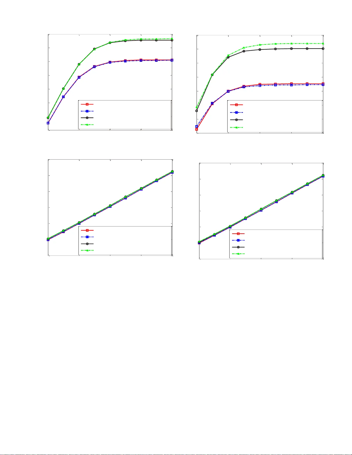
1 Massi v e MIMO Relaying with Linear Precoding in Correlate d Channels under Limited Feedback Y ang Liu † , Zhiguo D ing , Jia Shi, W eiwei Y ang an d Ping Zhong Abstract —In this paper we stu dy on a massiv e MIMO relay system with linear precoding under the cond itions of imperfect channel state information at the transmitter (CSIT) and per - user channel transmit corr elation . In our system the source-relay channels are ma ssive multiple-inpu t multiple-outp ut (MIM O) ones and the relay-destination channels are massi ve multipl e- input sin gle-output (MISO) ones. Large random matrix theory (RMT) is used to derive a deterministic equivalent of the signal- to-interference-plus-noise ratio (S INR) at each user in massiv e MIMO amplify-forward and decode-f orward (M-MIM O-ADF) relaying with regularized zero-fo rcing (RZF) precoding, as the number of transmit antennas and users M , K → ∞ and M ≫ K . In this paper we obt ain a closed-form expression f or th e deterministic equivalent of h H k ˆ W l ˆ h k , and w e give two theorems and a corollary to derive the deterministic equivalent of the SINR at each user . Simulation results show that the deterministic equivalent of the SINR at each user in M-MIMO-ADF relaying and the results of Theorem 1, T heorem 2, Proposition 1 and Corollary 1 are accurate . Index T erm s —Massive MIMO, relay , linear preco ding, random matrix theory (RM T), deterministic equ iv alent. I . I N T RO D U C T I O N I N recent years massi ve multiple-input multiple-outpu t (MIMO) an te n na system has be come a key pillar in the research of the 5th gen eration (5G) wireless co mmunica tion technolog ies. As compared to con ventional MIMO systems, massi ve MIMO systems can bring sev eral orders of mag- nitude gain to spectral an d energy efficiency [1]-[ 4]. It has been p roved that the sum capacity of multi-user massive MIMO (MU-M - MIMO) channels can b e greatly enhanced as co mpared to that of single u ser massiv e MIM O (SU-M- MIMO) channels. However , MU-M- MIMO suffers f rom pilot contamina tio n (i.e., re sidual interference which is caused by the reuse of pilot sequences in adjac e nt cells) [5 ], inter-user interferen ce at rece ivers [6 ][7], and imp e rfect ch annel state informa tio n (CSI) acquisition [8][9], etc. T o mitigate inter-user interferen ces, appropr iate precoding is needed at transmitters. As we know , dirty-paper coding (DPC) is a ca p acity ach ieving p recoding strategy for th e G a ussian MIMO b roadcast chann e ls (MIMO-BC) [ 10][11 ]. Howe ver, Y . Liu † (e-mail: ly@bupt.edu.cn ) is with the School of E lectro nic Engineeri ng, Beijing Univ ersity of Posts and T elecommunic ations, Beijing 100876, China. Z. Ding is with the School of Computing and Communicat ions, Lancaster Uni versi ty , Lancaster , LA1 4W A, UK. J. Shi is with the Uni versit y of Surrey , Guildford, GU2 7XH, U K. W . Y ang is with the Colle ge of Communi cations Enginee ring, PLA Uni- versi ty of Science and T echnology , Nanjing, China. P . Zhong is with the Scho ol of Mathematics a nd Stat istics, Uni versity of W uhan, Wuha n 430074, China. P . Zhong is also with the Department of Pure Mathemat ics, Univ ersity of W aterloo, W aterloo, Ontari o, Canada N2L 3G1. DPC preco der is nonlinear and it is much mor e complex to be implemen ted for practical use. For a massive MIMO system with large number of antennas, lo w-complexity linear precod in g such as zero -forcing (ZF) [11][ 12] and regularized zero-fo rcing (RZF) can achiev e near-optimal rate p erform a n ce and thus is mo re suitable for practical use. On the o ther hand, precod in g fo r massiv e MI MO systems require s acc u rate in - stantaneous ch annel state inform ation at the transmitter (CSIT) which is untenable in practice, and the inaccuracy of CSIT will seriously a ffect th e perf ormance of massive MIM O systems. For th is reason, many research works study on massi ve MI MO systems with imperfect CSIT [13][ 14][2 1][22][26]. Besides d irect tra nsmission, many r esearch works also stud y on the application of m assi ve MIMO to cooperative relay systems, e.g. , there ha ve been som e works o n multi-way massi ve MIMO relay systems [15][16 ]. Th ese massive MIMO relay systems can offer th e benefits o f both massive MIM O and multi-way relay systems, thus are expe cted to achiev e very high spectr a l efficiency . One of the disadvantages of massive MIMO systems is the in creased hardware and software co m - plexity , which can be red uced by antenna selection a t base station (BS) o r relay s. Antenna selection h as been a key top ic in the field of massi ve MI MO research in the past yea rs, the use of antenna selection in transmission or reception also has the benefits of improving power ef ficiency and im proving system perfo rmance [1 7]-[1 9 ]. For a massive MIMO system with n umber of anten nas M → ∞ , if par tial CSI such as statistical CSI and channel correlation matrices are available, then a large system anal- ysis can be carried out and the signal-to -interfere nce-plus- noise ratio (SINR) can be appr oximated b y a deter m inistic equiv alent. Hoch wald et a l . [20] we r e the first to study on large system analysis with M , K → ∞ ( M an d K den ote the number of antennas and u sers, respecti vely) and finite ratio for linear precod ing. W agner et a l . [21] studied large system analy sis on the sum rate perfo rmance of ZF and RZF precoding for large multiple-inp ut sing le-outpu t (MISO) broadc a st systems u nder the con ditions o f imperfect CSIT and per-user channel transmit correlation. Besides, [22][2 3] analyzed a rate-sp litting (RS) and a h ierarchical-r ate-splitting (HRS) schem e for massiv e MI MO with imperf ect CSIT in a lar ge-scale array regime. [2 4] stu d ied a non-r egenerative massi ve MIMO non- orthog o nal multiple access (NOM A) relay system, in which SU- M-MIMO is applied betwe e n the BS and the relay w h ile MU-M-MIM O is applied b etween the relay and the users. Large system analysis for massive MIMO c a n also be found in [7][1 3][25 ][26][27]. In th is paper, we stud y on a massiv e MIM O relay system 2 with linea r precod ing under limited feedback , i.e., a BS equippe d with M ( M → ∞ ) antennas co mmunicate s K single-anten na no n-coop erative receiv ers with the help o f a relay equipped with M + K antenn as. W e co nsider RZF precod in g under th e con ditions of imperfec t CSIT and per-user channel transmit co rrelation, a nd the relay schemes are b ased on h alf-dup lex am plify-fo rward (AF) or d ecode-fo rward (DF) mode. T he main c o ntributions of this paper can be summarized as follows: • For m assi ve MIMO AF an d DF (M-MIMO-ADF) r e - laying with RZF preco ding under th e conditions of im- perfect CSIT , per-user channe l correlation , and that th e source-re la y channels are massive MIMO ones r ather than massi ve MISO ones, we approx imates the SINR at each user by a deterministic equivalent. T his pap er is one of the few w orks in volving de te r ministic approximation s for precod ing in massiv e MIMO ch a n nels (rather than massi ve MISO ch annels). Compared with SU-M-MIM O or MU-M-MIMO method, our metho d can make a real system easy to be synchron ized. • Under the conditions of imperfect CSIT a n d per-user channel tra n smit corr elation, we gi ve two theo rems and a corollary to derive the deterministic equiv alent of the SINR at each user; and different fro m th e iterative method in [21 ] to obtain th e deterministic equiv alent o f h H k ˆ W l ˆ h k , we obtain a closed-fo rm expression for the deterministic equiv a le n t of h H k ˆ W l ˆ h k . • Simulation results match well with th eoretical analy sis. It sho ws that the determ inistic equ ivalent of the SINR at each u ser in M-MIMO-ADF relay in g an d the results of Theorem 1, T heorem 2, Proposition 1 and Corollary 1 are accurate. The rest of th is paper is o rganized as follows. System mo del and scheme descrip tion is introd uced in Section II . Section III derives the d e terministic eq uiv a lent of the SI N R at eac h user u n der the co nditions of imperfect CSIT and common correlation . Simulation results are giv en in Section IV . Finally , conclusion s ar e summarized in Section V . The proof s for Theorem 1 , Theorem 2, Proposition 1 and Corollary 1 are pre sen ted in Append ix A, B, and C r espec- ti vely , an d some lemmas which are used in our proof s are collected in Appendix D. N otation : In the following, b oldface lower-case and upper- case characters denote v ectors and matrices, resp e cti vely . The operator s ( · ) H , ( · ) T , tr ( · ) and E [ · ] de note con jugate transpose, transpose, trace and expectatio n, respectively . I M denotes the M × M identity matrix . log ( · ) is the natu ral logarithm. I I . S Y S T E M M O D E L A N D S C H E M E D E S C R I P T I O N A. System Model Consider a do wnlink transmission scen a r io with o ne BS transmitting data to multiple users with the h elp of a sin- gle relay . The BS sends indep endent user symbols s = [ s 1 , · · · , s K ] T to K users, wh ere the da ta s k is for the k - th user ( k ∈ { 1 , 2 , · · · , K } ). The BS is e q uipped with M antennas, each user is equip ped with a sing le antenna. It is assumed there is no d irect link between the BS and the users. S    Base Statio n 1 M R    Rel ay 1 M    1 K    2 2 D 1 D 2 D K 2 Fig. 1. System model. The relay works in ha lf -duplex mo de and is eq u ipped with M + K antennas, where M is the nu mber o f transmit antennas, and K is the num ber of recei ve an tennas of the relay . In this paper a large sy stem analy sis is carried out with M → ∞ , K → ∞ for M ≫ K . He re M → ∞ means that the BS a nd the relay are eq uipped with hund r eds of tran smit antennas. Besides, M ≥ K is assum ed to m ake u ser scheduling not have to be analy zed. Please note that a massiv e MIMO relay system ma y be sensitiv e to delay , e.g., massive MIMO relayin g in a vehicle n etwork. As co m pared to decodin g with all the receive antenna s of the relay , the first hop decoding with K receive antennas o f the relay is a m ore sim p le task and may be acco mplished with less delay . Besides, such a system setup (that the relay uses small numbe r ( K ) of anten nas to re ceiv e signals, and th en uses ma ny ( M ) antennas to tr ansmit signals) is a balan ced setup for the first (BS → relay) and the secon d hop (r elay → users) o f the relay system, wh ich can achieve both large s um rate and low delay . W ith a RZF precodin g, th e transm itted signal at the BS is x s = K X k =1 √ p s,k g sr ,k s k (1) where g sr ,k ∈ C M denotes the precod in g vector for a source- relay chan nel from the BS to the k -th receive antenna of th e relay , p s,k denotes the transm it p ower for symb ol s k , P is the transmit power co n straint for the BS or the relay . In this system each channel is modele d as h ij,k = √ M Θ 1 / 2 ij,k z ij,k (2) where ij ∈ { sr , rd } , sr and r d denotes a sou r ce-relay and a relay-destina tion channel respecti vely , k ∈ { 1 , · · · , K } , Θ ij,k denotes the chan n el cor relation matrix which is assumed to be slowly varying as co mpared to the channel coh erence time and thus are supposed to b e perfectly known to the transmitter, z ij,k ∼ C N (0 , 1/ M ) den o tes the q uasi-static independen t and identically distributed (i.i.d .) fast fadin g chann e l vector . User k is assumed to ha ve only kno wledge ab out Θ ij,k . Moreover , only an impe r fect estimated channel of ˆ h ij,k is assumed to be av ailab le at the tra n smitter and the relay which is modeled as ˆ h ij,k = √ M Θ 1 / 2 ij,k  q 1 − τ 2 ij,k z ij,k + τ ij,k q ij,k  = √ M Θ 1 / 2 ij,k ˆ z ij,k (3) 3 where ˆ z ij,k = q 1 − τ 2 ij,k z ij,k + τ ij,k q ij,k , q ij,k ∼ C N (0 , 1/ M ) is ind ependen t of z ij,k , τ ij,k ∈ [0 , 1] r eflects the accur acy of channel estimation. B. Scheme Description Next we in troduce the transmission scheme. Let the RZF precod in g vector be g sr ,k = ξ 1 ˆ W 1 ˆ h sr ,k , g r d,k = ξ 2 ˆ W 2 ˆ h r d,k , (4) where ˆ W 1 =  ˆ H H 1 ˆ H 1 + M α 1 I M  − 1 ∈ C M × M , ˆ H 1 = h ˆ h sr , 1 , · · · , ˆ h sr ,K i H ∈ C K × M , ˆ h sr ,k , ˆ h r d,k ∈ C M , ˆ W 2 =  ˆ H H 2 ˆ H 2 + M α 2 I M  − 1 ∈ C M × M , ˆ H 2 = h ˆ h r d, 1 , · · · , ˆ h r d,K i H ∈ C K × M , ξ 2 = ξ AF for AF relay ing, and ξ 2 = ξ DF for DF relaying. In th e first time slot, the r eceiv ed signal at the relay is given by y sr = H sr x s + n r =     h H sr , 1 . . . h H sr ,K     " K X k =1 s Gp s,k r α sr g sr ,k s k # +     n r, 1 . . . n r,K     =      h H sr , 1 q Gp s, 1 r α sr g sr , 1 . . . h H sr ,K q Gp s, 1 r α sr g sr , 1      s 1 +      h H sr , 1 q Gp s, 2 r α sr g sr , 2 . . . h H sr ,K q Gp s, 2 r α sr g sr , 2      s 2 + · · · +      h H sr , 1 q Gp s,K r α sr g sr ,K . . . h H sr ,K q Gp s,K r α sr g sr ,K      s K +     n r, 1 . . . n r,K     (5) where H sr = [ h sr , 1 , · · · , h sr ,K ] H ∈ C K × M denotes the i.i.d. channel matrix from the BS to the relay , h sr ,k ∈ C M ( k ∈ { 1 , · · · , K } ) d e n otes the i.i.d. ch a n nel vector from the BS to the k -th receive antenn a of the relay; r sr is th e distance from the BS to the relay; α is th e path loss exponen t, G is a constant that in corpor ates th e e ffects of path loss, antenna gain, antenna height, an d o ther factors; n r denotes the additi ve white Gaussian noise ( A WGN) vector at the relay , n r,k ∈ C N (0 , N 0 ) d enotes the A WGN at the k -th r eceiv e antenna of the re la y . Then the received signal at the k -th recei ve antenna of the relay is given by y sr ,k = h H sr ,k K X n =1 s Gp s,n r α sr g sr ,n s n + n r,k (6) Before we move o n to the next discussion, let’ s introd uce the following theorem which is useful for the subsequ ent large system analysis. Theor em 1: Let Φ = { h sr , 1 , · · · , h sr ,K , h r d, 1 , · · · , h r d,K } , ˆ Φ = n ˆ h sr , 1 , · · · , ˆ h sr ,K , ˆ h r d, 1 , · · · , ˆ h r d,K o , h k ∈ Φ , ˆ h k ∈ ˆ Φ , ˆ h k ′ ∈ ˆ Φ − ˆ h k , then we have    h H k ˆ W l ˆ h k    ≫    h H k ˆ W l ˆ h k ′    for any k 6 = k ′ , M → ∞ and M ≫ K , where k , k ′ ∈ { 1 , · · · , K } and l ∈ { 1 , 2 } . Pr oof: The proof of Theorem 1 is gi ven in Appendix A.  Since it is assumed that each recei ver has only infor mation about th e c h annel co rrelation m atrices and the statistical CSI, the conventional sing ular value decomposition (SVD) of channel m atrices cann ot be applied to MIMO data decodin g. Thus, in this paper only the received signal at the k -th receive antenna o f the relay is used to calculate the received SINR of sym bol s k , and successiv e inter ference cancellation (SIC) cannot be app lied to data decod ing. Therefo re the interfere n ce to symb ol s k cannot b e cance lled and the received SINR for symbol s k at the relay is given by γ sr ,k = Gp s,k r α sr    h H sr ,k g sr ,k    2 K P j =1 ,j 6 = k Gp s,j r α sr    h H sr ,k g sr ,j    2 + N 0 (7) In th e seco nd time slot, the BS keeps silent, the relay can either a mplify or decode the received sign al and forward it to the users. 1) Amplify-a nd-F orward: For AF relay ing, in the second time slot the transmitted signal vector at the relay is x r = K X m =1 √ p r,m g r d,m h H sr ,m K X n =1 s Gp s,n r α sr g sr ,n s n ! + n r,m ! , (8) and the receiv ed signal vector at the u sers is giv en by y r d = H r d x r + n d =    h H r d, 1 . . . h H r d,K    " K X m =1 s Gp r,m r α r d g r d,m h H sr ,m K X n =1 s Gp s,n r α sr g sr ,n s n ! + n r,m ! # +    n d, 1 . . . n d,K    (9) Thus in the second time slot the received signal at user k is y r d,k = h H r d,k K X m =1 s Gp r,m r α r d g r d,m h H sr ,m K X n =1 s Gp s,n r α sr g sr ,n s n ! + n r,m ! ! + n d,k = h H r d,k s Gp r, 1 r α r d g r d, 1 h H sr , 1 K X n =1 s Gp s,n r α sr g sr ,n s n ! + · · · + s Gp r,K r α r d g r d,K h H sr ,K K X n =1 s Gp s,n r α sr g sr ,n s n ! + s Gp r, 1 r α r d g r d, 1 n r, 1 + · · · + s Gp r,K r α r d g r d,K n r,K ! + n d,k . (10) Then within two time slots the received SINR at user k is expressed as Eq . ( 11), and the average tran smission rate f or user k is restricted by R AF k ≤ 1 2 log  1 + γ AF k  . (12) 4 γ AF k = γ AF r d,k =     h H r d,k  K P m =1 q Gp r,m r α rd g r d,m h H sr ,m q Gp s,k r α sr g sr ,k      2      h H r d,k K P m =1 q Gp r,m r α rd g r d,m h H sr ,m K P j =1 ,j 6 = k q Gp s,j r α sr g sr ,j !      2 +     h H r d,k  K P m =1 q Gp r,m r α rd g r d,m      2 N 0 + N 0 M → ∞ − − − − → Gp s,k r α sr × Gp r,k r α rd    h H r d,k g r d,k    2    h H sr ,k g sr ,k    2   Gp r,k r α rd    h H r d,k g r d,k    2 K P j =1 ,j 6 = k Gp s,j r α sr    h H sr ,k g sr ,j    2 +      h H r d,k K P j =1 ,j 6 = k q Gp r,j r α rd g r d,j h H sr ,j q Gp s,j r α sr g sr ,j      2   + Gp r,k r α rd    h H r d,k g r d,k    2 N 0 + N 0 (11) 2) Decod e-and- F orwar d : In the secon d time slo t, the BS keeps silent, the relay decodes and forwards the rec eiv ed signal to the users. The transmitted signal vector at the relay is x r = K X n =1 √ p r,n g r d,n s n , (13) and the receiv ed signal vector at the users is gi ven by y r d = H r d x r + n d =    h H r d, 1 . . . h H r d,K    " K X n =1 s Gp r,n r α r d g r d,n s n # +    n d, 1 . . . n d,K    =        h H r d, 1  K P n =1 q Gp r,n r α rd g r d,n s n  . . . h H r d,K  K P n =1 q Gp r,n r α rd g r d,n s n         +    n d, 1 . . . n d,K    (14) Thus in the second time slot the received signal at user k is y r d,k = h H r d,k K X n =1 s Gp r,n r α r d g r d,n s n ! + n d,k , (15) and the receiv ed SINR at user k is given b y γ DF r d,k = Gp r,k r α rd    h H r d,k g r d,k    2 K P n =1 ,n 6 = k Gp r,n r α rd    h H r d,k g r d,n    2 + N 0 (16) Then within two time slots the received SINR at u ser k is expressed as γ DF k = min  γ DF sr ,k , γ DF r d,k  = min          Gp s,k r α sr    h H sr ,k g sr ,k    2 K P n =1 ,n 6 = k Gp s,n r α sr    h H sr ,k g sr ,n    2 + N 0 , Gp r,k r α rd    h H r d,k g r d,k    2 K P n =1 ,n 6 = k Gp r,n r α rd    h H r d,k g r d,n    2 + N 0          (17) W ithin tw o time slo ts the average transm ission rate for u ser k is restricted by R DF k ≤ 1 2 log  1 + γ DF k  (18) I I I . D E T E R M I N I S T I C E Q U I V A L E N T F O R T H E S I N R This section discusses the deterministic ap- proxim a tion for the SINR at the users. Let Φ = { h sr , 1 , · · · , h sr ,K , h r d, 1 , · · · , h r d,K } , ˆ Φ = n ˆ h sr , 1 , · · · , ˆ h sr ,K , ˆ h r d, 1 , · · · , ˆ h r d,K o , h k ∈ Φ , ˆ h k ∈ ˆ Φ , before we deri ve the deterministic equi valent for the SINR at user k in M - MIMO-ADF relaying with RZF precod ing, let’ s first d erive the deter m inistic equ iv alen ts for th e following items: A. Deterministic Equivalent o f h H k ˆ W l ˆ h k , ˆ h H k ˆ W 2 l ˆ h k and K P j =1 ,j 6 = k    h H k ˆ W l ˆ h j    2 On how to obtain the deterministic equiv alent of h H k ˆ W l ˆ h k , ˆ h H k ˆ W 2 l ˆ h k and K P j =1 ,j 6 = k    h H k ˆ W l ˆ h j    2 for ∀ k ∈ { 1 , · · · , K } , l ∈ { 1 , 2 } , an d M ≫ K , let’ s first recall the results of [21]: h H k ˆ W l ˆ h k − q 1 − τ 2 k m o k 1 + m o k M →∞ − − − − → 0 , (19) ˆ h H k ˆ W 2 l ˆ h k − m ′ k M (1 + m o k ) 2 M →∞ − − − − → 0 , (20) K X j =1 ,j 6 = k    h H k ˆ W l ˆ h j    2 − Υ o k Φ k M →∞ − − − − → 0 , (21) almost surely , where m o k = 1 M tr   Θ 1/2 k  H Θ 1/2 k  T , (22) T =    1 M K X j =1  Θ 1/2 j  H Θ 1/2 j 1 + m o j + α l I M    − 1 , ( 23) 5 Υ o k = 1 M K X j =1 ,j 6 = k m ′ j,k  1 + m o j  2 , (24) Φ k = 1 − τ 2 k  1 − (1 + m o k ) 2  (1 + m o k ) 2 , (25) with m ′ = [ m ′ 1 , · · · , m ′ K ] T and m ′ k = [ m ′ 1 ,k , · · · , m ′ K,k ] T defined by m ′ = ( I K − J ) − 1 v , m ′ k = ( I K − J ) − 1 v k , (26) where J , v an d v k are given by [ J ] ij = 1 M tr   Θ 1/2 i  H Θ 1/2 i  T   Θ 1/2 j  H Θ 1/2 j  T M  1 + m o j  2 , (27) v =  1 M tr   Θ 1/2 1  H Θ 1/2 1  T 2 , · · · , 1 M tr   Θ 1/2 K  H Θ 1/2 K  T 2  T , (28) v k =  1 M tr  Θ 1/2 1 Θ 1/2 1  T  Θ 1/2 k Θ 1/2 k  T , · · · , 1 M tr  Θ 1/2 K Θ 1/2 K  T  Θ 1/2 k Θ 1/2 k  T  T (29) Different from the iterative method in [21] to obtain the deterministic equivalent of h H k ˆ W l ˆ h k , which may b e time- consumin g an d may n ot fu nction well f or a real ma ssi ve MIMO system, in this paper we o btain a closed- form expr es- sion for th e deterministic equivalent o f h H k ˆ W l ˆ h k . It req uires less com putation time an d is mo re practicable f or a real massi ve MIMO system which may be sensiti ve to delay . The f ollowing theorem and pro position are useful for the subsequen t large system analysis. Theor em 2: L e t ˆ Φ = n ˆ h sr , 1 , · · · , ˆ h sr ,K , ˆ h r d, 1 , · · · , ˆ h r d,K o , ˆ h k ∈ ˆ Φ , ˆ h k ′ ∈ ˆ Φ − ˆ h k , then we have    ˆ h H k ˆ W 2 l ˆ h k    ≫    ˆ h H k ˆ W 2 l ˆ h k ′    for a ny k 6 = k ′ , M → ∞ and M ≫ K , where k , k ′ ∈ { 1 , · · · , K } and l ∈ { 1 , 2 } . Pr oof: The pro of of Theorem 2 is gi ven in Appendix B.  Pr opo sition 1: Let Φ = { h sr , 1 , · · · , h sr ,K , h r d, 1 , · · · , h r d,K } , ˆ Φ = n ˆ h sr , 1 , · · · , ˆ h sr ,K , ˆ h r d, 1 , · · · , ˆ h r d,K o , h k ∈ Φ , ˆ h k ∈ ˆ Φ , then we have h H k ˆ W l ˆ h k − √ 1 − τ 2 k tr   Θ 1/2 k  H Θ 1/2 k  M α l + tr   Θ 1/2 k  H Θ 1/2 k  M →∞ − − − − → 0 for any M , K → ∞ and M ≫ K , wh ere k ∈ { 1 , · · · , K } and l ∈ { 1 , 2 } . Pr oof: The proof of Proposition 1 is given in Appen dix C.  B. T ransmit P o wer 1) T ransmit P ower Constr aint at the BS: T o satisfy the total transmit power constraint at the BS, th e precod in g vector s are normalized as K X k =1 p s,k g H sr ,k g sr ,k = K X k =1 p s,k ξ 2 1 ˆ h H sr ,k ˆ W 2 1 ˆ h sr ,k ≤ P ( 30) Then we hav e the following constraint f o r ξ 2 1 : ξ 2 1 − ( ξ o 1 ) 2 M →∞ − − − − → 0 (31) almost surely , where ( ξ o 1 ) 2 = P K P k =1 p s,k  m ′ sr,k M ( 1+ m o sr,k ) 2  (32) 2) T ransmit P ower Con straint at the Relay for AF Relaying: T o satisfy the total tran sm it po wer con straint for AF relaying, the pr ecoding vecto rs f or the transm itted signals at th e relay are normalized as K X m =1 p r,m g H r d,m g r d,m K X n =1     h H sr ,m Gp s,n r α sr g sr ,n     2 + N 0 ! M →∞ − − − − → ( a ) ξ 2 AF K X m =1 p r,m  ˆ h H r d,m ˆ W 2 2 ˆ h r d,m   Gp s,m r α sr ξ 2 1    h H sr ,m ˆ W 1 ˆ h sr ,m    2 + N 0  ≤ P (33) where (a) follows T heorem 1 . Th e n we have the following constraint for ξ 2 AF : ξ 2 AF − ( ξ o AF ) 2 M →∞ − − − − → 0 (34) almost surely , where ( ξ o AF ) 2 = P K P m =1 p r,m m ′ rd,m M ( 1+ m o rd,m ) 2  Gp s,m r α sr ( ξ o 1 ) 2 (1 − τ 2 m )  m o sr,m 1+ m o sr,m  2 + N 0  (35) 3) T ransmit P ower Constr aint at the Relay fo r DF Rela ying: T o satisfy the total tran sm it po wer con straint for DF relaying, the pr ecoding vecto rs f or the transm itted signals at th e relay are normalized as K X n =1 p r,n g H r d,n g r d,n = ξ 2 DF K X n =1 p r,n  ˆ h H r d,n ˆ W 2 2 ˆ h r d,n  ≤ P (36) Then we hav e the following constraint f o r ξ 2 DF : ξ 2 DF − ( ξ o DF ) 2 M →∞ − − − − → 0 (37) almost surely , where ( ξ o DF ) 2 = P K P n =1 p r,n m ′ rd,n M ( 1+ m o rd,n ) 2 (38) C. De terministic Equivalent for the SINR Cor ollary 1: Let Φ = { h sr , 1 , · · · , h sr ,K , h r d, 1 , · · · , h r d,K } , ˆ Φ = n ˆ h sr , 1 , · · · , ˆ h sr ,K , ˆ h r d, 1 , · · · , ˆ h r d,K o , h k ∈ Φ , ˆ h k ∈ ˆ Φ for any k 6 = k ′ , M → ∞ and M ≫ K wh ere k , k ′ ∈ { 1 , · · · , K } and l ∈ { 1 , 2 } , if the tran smit p ower for each user message at th e BS or the relay is equ a lly allocated as P / K , then the deterministic equ iv alen t f or th e recei ved SINR at u ser k in M-MIMO-ADF relaying is given by γ AF k −  γ AF k  o M →∞ − − − − → 0 (39) γ DF k −  γ DF k  o M →∞ − − − − → 0 (40) 6  γ AF k  o = G r α sr G r α rd  P K  2 ( ξ o 1 ) 2 ( ξ o AF ) 2 Γ 2 sr ,k Γ 2 r d,k G r α rd G r α sr  P K  2 ( ξ o 1 ) 2 ( ξ o AF ) 2 Γ 2 r d,k Υ o sr ,k Φ sr ,k + G r α sr G r α rd  P K  2 ( ξ o 1 ) 2 ( ξ o AF ) 2 Γ 2 sr ,k Υ o r d,k Φ r d,k + G r α rd P K ( ξ o AF ) 2 Γ 2 r d,k N 0 + N 0 (41)  γ DF k  o ≤ min    G r α sr P K ( ξ o 1 ) 2 Γ 2 sr ,k G r α sr P K ( ξ o 1 ) 2 Υ o sr ,k Φ sr ,k + N 0 , G r α rd P K ( ξ o DF ) 2 Γ 2 r d,k G r α rd P K ( ξ o DF ) 2 Υ o r d,k Φ r d,k + N 0    (42) almost surely , wher e  γ AF k  o and  γ DF k  o are given by Eq. (41) and Inequality (42) with Γ sr ,k = q 1 − τ 2 k tr  Θ 1/2 k  H Θ 1/2 k M α 1 + tr  Θ 1/2 k  H Θ 1/2 k , (43) Γ r d,k = q 1 − τ 2 k tr  Θ 1/2 k  H Θ 1/2 k M α 2 + tr  Θ 1/2 k  H Θ 1/2 k , (44) Υ o sr ,k and Υ o r d,k are defined as Eq. (24), Φ sr ,k and Φ r d,k are defined as Eq. (25), ( ξ o 1 ) 2 , ( ξ o AF ) 2 , ( ξ o DF ) 2 are d efined in Eq. (32), Eq. (35), Eq. (38), respectively . Pr oof: Please note that th e deriv ed SIN Rs have to be av eraged over to get the ergodic ones. Eq . (4 1) can be obtained from Eq. (11 ) and section II I. (A)(B), and the two term s in the m in {} operato r of Inequ ality (42) can be o btained from Eq. (17) and section II I. (A)(B). Next we complete the proof of Ineq uality (42) to show that the minimu m one o f the two terms in the min {} operator is a lo wer bou nd for  γ DF k  o : Applying The o rem 1 we h av e    h H k ˆ W l ˆ h k    ≫    h H k ˆ W l ˆ h k ′    if the assumption ho lds true (for any k 6 = k ′ , M → ∞ and M ≫ K where k , k ′ ∈ { 1 , · · · , K } and l ∈ { 1 , 2 } ) . Fro m Eq. (49 ) and Eq. ( 50) of App endix A, if th e signal ch annel coefficient ↑    h H k ˆ W l ˆ h k    → t    h H k ˆ W l ˆ h k    for ∀ t > 1 , then the interferen ce channe l coefficient ↑    h H k ˆ W l ˆ h k ′    will b e far less than t    h H k ˆ W l ˆ h k ′    , so that we have the following inequality: ϕ  X =    h H k ˆ W l ˆ h k     = GP K    h H k ˆ W l ˆ h k    2 K P n =1 ,n 6 = k GP K    h H k ˆ W l ˆ h n    2 + N 0 ≤ GP K t    h H k ˆ W l ˆ h k    2 K P n =1 ,n 6 = k GP K t    h H k ˆ W l ˆ h n    2 + N 0 = ϕ  X = √ t    h H k ˆ W l ˆ h k     , (4 5 ) which pr oves that ϕ ( X ) is a mon otone increasing quasi- concave function . Besides, from E q . (49) and Eq. (50) of Append ix A, X =    h H k ˆ W l ˆ h k    can b e seen as a mo notone increasing concave fun ction, while Y =    h H k ˆ W l ˆ h k ′    can be seen as a constant if the assum ption ho lds true, therefo re it further proves that ϕ ( X ) is a mo notone increasing con cav e function . Since γ DF sr ,k ( X ) an d γ DF r d,k ( X ) h as th e same form as ϕ ( X ) so that they are both co n cave fu n ctions if the assumption h olds true, then f or ∀ θ ∈ [0 , 1] we have the following inequality: γ DF k ( θX 1 + (1 − θ ) X 2 ) = min  γ DF sr ,k ( θX 1 + (1 − θ ) X 2 ) , γ DF r d,k ( θX 1 + (1 − θ ) X 2 )  ≥ min  θγ DF sr ,k ( X 1 ) + ( 1 − θ ) γ DF sr ,k ( X 2 ) , θγ DF r d,k ( X 1 ) + (1 − θ ) γ DF r d,k ( X 2 )  ≥ θ min  γ DF sr ,k ( X 1 ) , γ DF r d,k ( X 1 )  + (1 − θ ) min  γ DF sr ,k ( X 2 ) , γ DF r d,k ( X 2 )  = θ γ DF k ( X 1 ) + ( 1 − θ ) γ DF k ( X 2 ) , (46) which p roves that γ DF k ( X ) is a concav e fun ction if the assumption holds true. Fr om Jensen’ s inequality an d the c o n- cavity of γ DF k ( X ) it leads to the inequ ality E  γ DF k ( X )  ≤ γ DF k ( E ( X )) if the assumption holds true, which c ompletes the proof.  I V . S I M U L AT I O N R E S U LT S In this section, Monte-Carlo (MC) simulation results are compare d with large system ap proxim ations to validate the accuracy o f the der i ved deterministic equiv alents, and demon - strate the perfo rmance of the prop osed massive MIMO relay system. By assuming a diffuse 2 -D field of isotro pic scatterers around the receivers, th e correlatio n between the chan nel coefficients of antennas 1 ≤ i, j ≤ M of the k -th user is modeled as in [28] and is giv en by [ Θ k ] ij = 1 θ k, max − θ k, min Z θ k, max θ k, min e i 2 π λ d i,j cos( θ ) dθ (47) where λ denotes the signal wavelength, d i,j is the distance between tran smit anten nas i an d j , θ k is th e azimuth angle o f user k with respect to the or ientation perpe ndicular to the array axis, θ k, max − θ k, min indicates the angu lar spread of depar tu re to user k . Oth er system param e ters for performan ce ev aluation are giv en in T able I . Fig. 2 compare s the maximum sum rate of M-MIMO-ADF relaying by th e MC simulation to that b y the d eterministic approx imation with RZF precoding in correlate d chan nels ( M = 768 , K = 64 , Θ k 6 = I M ∀ k ). From Fig. 2(a) and Fig. 2(b), we observe that for both imperfect CSIT ( τ 2 k = 0 . 1 ) and per fect CSIT ( τ 2 k = 0 ), th e deterministic ap proxim ation achieves a lm ost the same su m rate as the MC result. Fro m Fig. 2(a), we see that the sum rate of M-MIMO-ADF relaying increases with the gr owth of transmit power , and it approa ches a con stant at h igh SNR region. This is bec ause with th e increasing tr ansmit p ower , the multi-u ser interfer ence becomes 7 T ABLE I S Y S T E M P A R A M E T E R S Parameters V alue Channel bandwidth 10 [MHz] Thermal noise d ensity -174 [dBm] Regularization parameter α 1 = α 2 = K /(10 M ρ ) Path-loss model L = 10lo g 10 ( d n / G ) , d in meter L = 128 . 1 + 37 . 6log 10 D , D in kilometer G = 0 . 029512 , n = 3 . 76 Distance d sr = 2500 [m], d r d = 1500 [m] much h ig her than the noise at th e k -th user, thu s th e sum rate of M-MIMO- ADF re laying is limited b y the multi-user interferen ces a t h igh SNR. Besides, we also find that the gap between the sum rate of M-MIMO-DF b y MC and tha t by deterministic ap proxima tion is greater th an the gap between the sum rate o f M-MIMO-AF by MC and that by deterministic approx imation, this is du e to the fact th at the sum rate of M-MIMO-DF re laying by dete r ministic appro ximation is an ergodic sum channel capacity in nature, whereas the su m rate of M-MIMO-DF relaying by MC is a minim u m sum chan nel capacity of s ource - relay and relay-destination channels. From Fig. 2( b), we see that the sum r ate of M-MIMO-ADF re laying increases with the growth of SNR, and the sum rate is propo rtional to the SNR. T he reason is that f o r perfec t CSIT ( τ 2 k = 0 ), the multi-user interfe r ence approac h es to zero with RZF p recoding , and from Eq. ( 11) and Eq . (17 ) we find that the sum rate should be propo rtional to the S NR. Fig. 3 comp ares the maximu m sum rate of the M- MIMO- ADF relayin g by the MC simulation to th at by the d eter- ministic approxim ation with RZF precoding in unco rrelated channels ( M = 768 , K = 64 , Θ k = I M ∀ k ). It can b e observed that for both imp erfect C SIT ( τ 2 k = 0 . 1 ) an d perfec t CSIT ( τ 2 k = 0 ) , the determ inistic app r oximation match es well with the M C results. Comparing Fig. 3(a) to Fig. 2(a), it can b e f ound th at the ma x imum sum rate of M-MI M O-ADF relaying for uncorrelated chan nels is much higher than that for correlated channe ls. Fig. 4 comp ares the maximu m sum rate of the M- MIMO- ADF r elaying by the M C simulatio n to that by the d eterminis- tic approx imation with RZF precoding in correlated chan nels ( M = 25 6 , K = 32 , Θ k 6 = I M ∀ k ). It c an be observed that if M and K ar e red uced to M = 2 56 and K = 32 , the deterministic approxim ation matches well with the MC result for both imper fect CSIT ( τ 2 k = 0 . 1 ) and per fect CSIT ( τ 2 k = 0 ). Howe ver, the g ap between the MC result an d the d eterministic approx imation become s larger as comp ared to that in Fig. 3, since the deterministic approxima tion by Eq. (19) and Eq. (20) becomes less accurate for a smaller M . Fig. 5 comp ares the maximu m sum rate of the M- MIMO- ADF relayin g by the MC simulation to that b y determin istic approx imation with RZF p r ecoding in uncorr elated ch a nnels ( M = 25 6 , K = 32 , Θ k = I M ∀ k ). It c an be observed that if M and K ar e red uced to M = 2 56 and K = 32 , the deterministic approxim ation matches well with the MC result for both imper fect CSIT ( τ 2 k = 0 . 1 ) and per fect CSIT ( τ 2 k = 0 ). Comparing Fig. 5(a) to Fig. 4( a), we fin d that the ma x imum 2 0 3 0 4 0 5 0 6 0 9 0 1 0 0 1 1 0 1 2 0 1 3 0 1 4 0 1 5 0 Tran s m i t po w er [dBm ] Maximu m sum rat e [bp s/Hz ] A F b y M o n te - Ca r lo A F b y d e te r ministi c a pp ro xima t io n DF by Monte -Ca rl o DF by d e te r min is ti c a pp r o xima t io n (a) τ 2 k = 0 . 1 2 0 3 0 4 0 5 0 6 0 1 0 0 2 0 0 3 0 0 4 0 0 5 0 0 6 0 0 Tran s m i t po w er [dBm ] Maximu m sum rat e [bp s/Hz ] A F b y M o n te - Ca r lo A F b y d e te r ministi c a pp ro xima t io n DF by Monte -Ca rl o DF by d e te r min is ti c a pp r o xima t io n (b) τ 2 k = 0 Fig. 2. Maxi mum s um rate ver sus transmit power with M = 768 , K = 64 , Θ k 6 = I M ( d i,j = 0 . 5 λ ) . sum rate of M- MIMO-ADF relay in g with RZF preco ding in uncorr elated chann els is much higher than that in correlated channels. From Fig. 2 - Fig. 5 we conc lude that the deter ministic approx imation fo r the received SINR at user k in the M- MIMO-ADF relaying and the results of Theo rem 1, Theorem 2, Proposition 1 and Corollary 1 are accurate. Fig. 6 and Fig. 7 compar e the MC result of h H k W 1 ˆ h k to the determ inistic equiv alent in Eq. (1 9) of [21 ] and the deterministic equ iv alen t in Propo sition 1 for the M-MIMO - ADF relayin g with RZF preco ding in both c o rrelated chann els ( M = 768 , K = 6 4 , Θ k 6 = I M ∀ k ) an d un correlated channels ( M = 768 , K = 64 , Θ k = I M ∀ k ). W e find that f or both imperfect CSIT ( τ 2 k = 0 . 1 ) and perf e c t CSIT ( τ 2 k = 0 ), the deterministic equivalent in E q. (19) and tha t in Prop osition 1 both match well with the MC result, and at low SNR region the matching for the dete r ministic eq uiv alen t in Proposition 1 8 2 0 3 0 4 0 5 0 6 0 8 0 1 0 0 1 2 0 1 4 0 1 6 0 1 8 0 2 0 0 2 2 0 Tran s m i t po w er [dBm ] Maximu m sum rat e [bp s/Hz ] A F b y M o n te - Ca r lo A F b y d e te r ministi c a pp ro xima t io n DF by Monte -Ca rl o DF by d e te r min is ti c a pp r o xima t io n (a) τ 2 k = 0 . 1 2 0 3 0 4 0 5 0 6 0 0 1 0 0 2 0 0 3 0 0 4 0 0 5 0 0 6 0 0 Tran s m i t po w er [dBm ] Maximu m sum rat e [bp s/Hz ] A F b y M o n te - Ca r lo A F b y d e te r ministi c a pp ro xima t io n DF by Monte -Ca rl o DF by d e te r min is ti c a pp r o xima t io n (b) τ 2 k = 0 Fig. 3. Maximum sum rate versus transmit po w er with M = 768 , K = 64 , Θ k = I M . is a little worse than that in Eq. (19). From Fig. 6 and Fig. 7, we co nclude that the deterministic equiv alent in Prop osition 1 matches well with th e MC result of h H k W 1 ˆ h k for both correlated an d uncorrelated ch annels if M , K → ∞ and M ≫ K . V . C O N C L U S I O N In th is p aper we studied a m a ssive MIMO r elay system with linear pr e coding a n d an alyzed the system performa n ce for a large number of antennas and users. Our chan nel mo del is realistic as the ch a n nels are assumed to have impe rfect CSIT and pe r-user chann el co rrelation, and ou r source-relay channels are massi ve MIMO ones rather than m assi ve MISO ones. W e u se large ran d om matrix theo ry ( RMT) to d erive the determin istic equivalent of the SINR at each u ser, as the number of transmit anten nas and the users M , K → ∞ a n d M ≫ K . Simulation results have shown th at the determin istic 2 0 3 0 4 0 5 0 6 0 3 5 4 0 4 5 5 0 5 5 6 0 6 5 7 0 Tran s m i t p o w er [dBm ] Maximu m su m rat e [bp s/Hz ] A F by Monte -Ca rl o A F by d e te r min is ti c a pp ro xima t io n DF by Monte- Ca rl o DF by d et e rminis ti c a pp r o xima ti o n (a) τ 2 k = 0 . 1 2 0 3 0 4 0 5 0 6 0 0 5 0 1 0 0 1 5 0 2 0 0 2 5 0 3 0 0 Tran s m i t po w er [dBm ] Maximu m sum rat e [bp s/Hz ] A F b y M o n te - Ca r lo A F b y d e te r ministi c a pp ro xima t io n DF by Monte -Ca rl o DF by d e te r min is ti c a pp r o xima t io n (b) τ 2 k = 0 Fig. 4. Maxi mum s um rate ver sus transmit power with M = 256 , K = 32 , Θ k 6 = I M ( d i,j = 0 . 5 λ ) . equiv alent o f the SINR at ea ch user in M-MIMO-ADF relay ing and the results of Theorem 1 , Theorem 2, Propo sition 1 an d Corollary 1 are accurate. As in practice individual chann el gains may no t b e a vailable for massive MIMO systems due to som e reasons such as lim- ited fee dback, p ilot con tamination, time- sen siti ve applicatio ns and so on , our large system perfor m ance a pprox imations can be applied to simulate the system behavior with o ut ha ving to carry ou t extensi ve MC simulations, and they can be used to solve practical o ptimization p roblems. Howe ver , a challengin g problem still remain s fo r future research on how to accu rately calculate th e determin istic equivalent o f the in terference to each user if M , K → ∞ an d the v alue of K is close to M . 9 2 0 3 0 4 0 5 0 6 0 2 0 3 0 4 0 5 0 6 0 7 0 8 0 9 0 1 0 0 Tran s m i t po w er [dBm ] Maximu m sum rat e [bp s/Hz ] A F b y M o n te - Ca r lo A F b y d e te r ministi c a pp ro xima t io n DF by Monte -Ca rl o DF by d e te r min is ti c a pp r o xima t io n (a) τ 2 k = 0 . 1 2 0 3 0 4 0 5 0 6 0 0 5 0 1 0 0 1 5 0 2 0 0 2 5 0 Tran s m i t po w er [dBm ] Maximu m su m rat e [bp s/Hz ] A F b y Mo n te - Ca r lo A F b y dete r ministi c a pp ro xima t io n DF by Monte -Ca rl o DF by d e te r min is ti c a pp r o xima t io n (b) τ 2 k = 0 Fig. 5. Maximum sum rate versus transmit po w er with M = 256 , K = 32 , Θ k = I M . A P P E N D I X A P R O O F O F T H E O R E M 1 W itho ut loss of generality , let’ s first p rove    h H k ˆ W 1 ˆ h k    ≫    h H k ˆ W 1 ˆ h k ′    . As we kn ow , ˆ W 1 =  ˆ H H 1 ˆ H 1 + M α 1 I M  − 1 is a symm etric and positiv e definite m atrix, it can be decompo sed as ˆ W 1 = U H 1 Λ 1 U 1 , where Λ 1 = diag ( λ 1 , · · · , λ M ) is a M × M diagon al matrix containing M po siti ve eigenv alues of ˆ W 1 . As ˆ W − 1 1 = h ˆ h sr , 1 , · · · , ˆ h sr ,K i h ˆ h sr , 1 , · · · , ˆ h sr ,K i H + M α 1 I M = U H 1 ( Λ ′ 1 + M α 1 I M ) U 1 (48) where Λ ′ 1 = diag   λ ′ 1 , · · · , λ ′ K | {z } K , 0 , · · · , 0 | {z } M − K   , λ ′ m > 0 for ∀ m ∈ { 1 , · · · , K } . Th en ˆ W 1 =  ˆ H H 1 ˆ H 1 + M α 1 I M  − 1 2 0 3 0 4 0 5 0 6 0 0 .92 0 .93 0 .94 0 .95 0 .96 0 .97 Tran s m i t p o w er [dBm ] h H k W 1 ^ h k Monte -Ca rl o Dete r minist ic equ iv a l e n t in Eq . (1 9 ) Dete r minist ic equ iv a l e n t in P ro pos i ti o n 1 (a) τ 2 k = 0 . 1 2 0 3 0 4 0 5 0 6 0 0 .97 0 .97 5 0 .98 0 .98 5 0 .99 0 .99 5 1 1 .00 5 Tran s m i t p o w er [dBm ] h H k W 1 ^ h k Monte -Ca rl o Dete r minist ic equ iv a l e n t in Eq . (1 9 ) Dete r minist ic equ iv a l e n t in P ro pos i ti on 1 (b) τ 2 k = 0 Fig. 6. h H k W 1 ˆ h k versus transmit powe r with M = 768 , K = 64 , Θ k 6 = I M ( d i,j = 0 . 5 λ ) . can be decomposed as ˆ W 1 = U H 1 Λ 1 U 1 , where Λ 1 = diag ( λ 1 , · · · , λ K , λ K +1 · · · , λ M ) is a M × M diagonal matrix containing M positiv e eig en values of ˆ W 1 , λ m = ( λ ′ m + M α 1 ) − 1 > 0 for m ∈ { 1 , · · · , K } and λ m = ( M α 1 ) − 1 > 0 for m ∈ { K + 1 , · · · , M } . Let U 1 Θ 1/2 k z k , [ x 1 , x 2 , · · · , x M ] T , U 1 Θ 1/2 k ′ z k ′ , [ y 1 , y 2 , · · · , y M ] T where x m and y m ( m ∈ { 1 , 2 , · · · M } ) follows th e same distribution, if the a c c uracy parameter o f the chann e l estimate satisfies th e following conditio n as τ = 10 2 0 3 0 4 0 5 0 6 0 0 .85 0 .87 0 .89 0 .91 0 .93 0 .95 Tran s m i t po w er [dBm ] h H k W 1 ^ h k Monte -Ca rl o Dete r minist ic equ i v a l e n t in E q. (1 9 ) Dete r minist ic equ i v a l e n t in Pro pos it io n 1 (a) τ 2 k = 0 . 1 2 0 3 0 4 0 5 0 6 0 0 .9 0 .92 0 .94 0 .96 0 .98 1 Tran s m i t po w er [dBm ] h H k W 1 ^ h k Monte -Ca rl o Dete r minist ic equ i v a l e n t in E q. (1 9 ) Dete r minist ic equ i v a l e n t in Pro pos it io n 1 (b) τ 2 k = 0 Fig. 7. h H k W 1 ˆ h k versus transmit powe r with M = 768 , K = 64 , Θ k = I M . τ k = τ k ′ , then we have h H k ˆ W 1 ˆ h k M →∞ − − − − → h H k U H 1 Λ 1 U 1 ˆ h k M →∞ − − − − → M  1 − τ 2  z H k  Θ 1/2 k  H U H 1 Λ 1 U 1 Θ 1/2 k z k + M τ p 1 − τ 2 z H k  Θ 1/2 k  H U H 1 Λ 1 U 1 Θ 1/2 k q k M →∞ − − − − → M  1 − τ 2  M X m =1 λ m | x m | 2 + M τ p 1 − τ 2 z H k  Θ 1/2 k  H U H 1 Λ 1 U 1 Θ 1/2 k q k (49) h H k ˆ W 1 ˆ h k ′ M →∞ − − − − → h H k U H 1 Λ 1 U 1 ˆ h k ′ M →∞ − − − − → M  1 − τ 2  z H k  Θ 1/2 k  H U H 1 Λ 1 U 1 Θ 1/2 k ′ z k ′ + M τ p 1 − τ 2 z H k  Θ 1/2 k  H U H 1 Λ 1 U 1 Θ 1/2 k ′ q k ′ M →∞ − − − − → M  1 − τ 2  M X m =1 λ m x H m y m + M τ p 1 − τ 2 z H k  Θ 1/2 k  H U H 1 Λ 1 U 1 Θ 1/2 k ′ q k ′ (50) As th e secon d terms in the above form ulas satisfy the follow- ing condition z H k  Θ 1/2 k  H U H 1 Λ 1 U 1 Θ 1/2 k q k − z H k  Θ 1/2 k  H U H 1 Λ 1 U 1 Θ 1/2 k ′ q k ′ M →∞ − − − − → 0 (51) and λ m > 0 , E ( x m ) = E ( y m ) = 0 , which means that λ m x H m y m has an equa l probability to be positi ve or negativ e, while λ m | x m | 2 is always positive. Fro m a statistical poin t of view , th e values of λ m   x H m y m   and λ m | x m | 2 are the same since x m and y m follows the same distribution. Theref ore the first terms in Eq. (49 ) and Eq. (50) satisfy th e following inequality M X m =1 λ m | x m | 2 − M X m =1 λ m   x H m y m   ≫ 0 , (52) for M → ∞ , th e n we h av e    h H k ˆ W 1 ˆ h k    ≫    h H k ˆ W 1 ˆ h H k ′    . Similarly , we can a lso prove    h H k ˆ W 2 ˆ h k    ≫    h H k ˆ W 2 ˆ h k ′    . So far we have proved that    h H k ˆ W l ˆ h k    ≫    h H k ˆ W l ˆ h k ′    for l ∈ { 1 , 2 } , the proof for Theorem 1 is complete. A P P E N D I X B P R O O F O F T H E O R E M 2 W itho ut loss of generality , le t’ s first prove    ˆ h H k ˆ W 2 1 ˆ h k    ≫    ˆ h H k ˆ W 2 1 ˆ h k ′    . If ˆ W 1 =  ˆ H H 1 ˆ H 1 + M α 1 I M  − 1 can be decom- posed as ˆ W 1 = U H 1 Λ 1 U 1 where Λ 1 = diag ( λ 1 , · · · , λ M ) is a M × M diagon a l matrix containing M positiv e eig en- values of ˆ W 1 , λ m > 0 for m ∈ { 1 , · · · , K } and λ m = ( M α 1 ) − 1 > 0 for m ∈ { K + 1 , · · · , M } , then ˆ W 2 1 =  ˆ H H 1 ˆ H 1 + M α 1 I M  − 2 is also a sym metric and positi ve definite matrix and can b e decomp osed a s ˆ W 2 1 = U H 1 Λ 2 1 U 1 , where Λ 2 1 = diag  λ 2 1 , · · · , λ 2 M  . Let U 1 ˆ h k , [ x 1 , x 2 , · · · , x M ] T , U 1 ˆ h k ′ , [ y 1 , y 2 , · · · , y M ] T where x m and y m ( m ∈ { 1 , 2 , · · · M } ) follows th e same distribution, th en we have ˆ h H k ˆ W 2 1 ˆ h k M →∞ − − − − → ˆ h H k U H 1 Λ 2 1 U 1 ˆ h k M →∞ − − − − → M X m =1 λ 2 m | x m | 2 (53) ˆ h H k ˆ W 2 1 ˆ h k ′ M →∞ − − − − → ˆ h H k U H 1 Λ 2 1 U 1 ˆ h k ′ M →∞ − − − − → M X m =1 λ 2 m x H m y m (54) 11 As λ 2 m > 0 and E ( x m ) = E ( y m ) = 0 , which mean s that both the real and th e imagin ary part of λ 2 m x H m y m have an equal proba b ility to b e positive or negative, while λ 2 m | x m | 2 is al ways p ositi ve. From a statistical point of vie w , th e values of λ 2 m   x H m y m   and λ 2 m | x m | 2 are the same since x m and y m follows the same distribution. From Eq. (53) and Eq. (54), the following inequality M X m =1 λ 2 m | x m | 2 − M X m =1 λ 2 m   x H m y m   ≫ 0 (55) holds fo r M → ∞ , then we have    ˆ h H k ˆ W 2 1 ˆ h k    ≫    ˆ h H k ˆ W 2 1 ˆ h k ′    . Similarly , we can p rove that    ˆ h H k ˆ W 2 2 ˆ h k    ≫    ˆ h H k ˆ W 2 2 ˆ h k ′    . So far we have proved that    h H k ˆ W 2 l ˆ h k    ≫    h H k ˆ W 2 l ˆ h k ′    for l ∈ { 1 , 2 } , the proof for Theorem 2 is complete. A P P E N D I X C P R O O F O F P RO P O S I T I O N 1 For any M , K → ∞ an d M ≫ K , wh ere k ∈ { 1 , · · · , K } and l ∈ { 1 , 2 } , let’ s d e r iv e the determ inistic equiv alent of h H k ˆ W l ˆ h k : h H k ˆ W l ˆ h k = h H k   ˆ h k ˆ h H k + K X j =1 ,j 6 = k ˆ h j ˆ h H j + M α l I M   − 1 ˆ h k M →∞ − − − − → tr  ˆ h k h H k  ˆ h k ˆ h H k + M α l I M  − 1  M →∞ − − − − → h H k ( M α l I M ) − 1 ˆ h k 1 + ˆ h H k ( M α l I M ) − 1 ˆ h k M →∞ − − − − → 1 M α l M z H k  Θ 1/2 k  H Θ 1/2 k  p 1 − τ 2 k z k + τ q k  1 + 1 α l  p 1 − τ 2 k z H k + τ q H k   Θ 1/2 k  H Θ 1/2 k  p 1 − τ 2 k z k + τ q k  M →∞ − − − − → p 1 − τ 2 k tr  Θ 1/2 k  H Θ 1/2 k M α l + tr  Θ 1/2 k  H Θ 1/2 k (56) Then we have h H k ˆ W l ˆ h k − p 1 − τ 2 k tr  Θ 1/2 k  H Θ 1/2 k M α l + tr  Θ 1/2 k  H Θ 1/2 k M →∞ − − − − → 0 (57) almost surely , and the proof for Proposition 1 is complete. A P P E N D I X D I M P O RTA N T L E M M A S Lemma 1 (Matrix In version Lemma): [29, Lemma 2.2]: Let U be an N × N invertible matr ix an d x ∈ C N , c ∈ C for which U + c xx H is in vertib le. Then x H  U + c xx H  − 1 = x H U − 1 1 + c x H U − 1 x . (58) Lemma 2 (Resolvent Identity): Let U and V be two invertible complex matrices of size N × N . Then U − 1 − V − 1 = − U − 1 ( U − V ) V − 1 . (59) Lemma 3 [ 30, Lemma 14.2]: L et A 1 , A 2 , · · · , with A N ∈ C N × N be a series of rando m matrices g enerated by the probab ility space (Ω , F , P ) such that, for w ∈ A ⊂ Ω , with P ( A ) = 1 , k A N ( w ) k < K ( w ) , u niformly on N . Let x 1 , x 2 , · · · , with x N ∈ C N , be rand om vecto rs of i. i. d. entries with zero mean, variance 1/ N , and eighth- order mome nt of order O  1  N 4  , indepen dent of A N . Then x H N A N x N − 1 N tr A N N →∞ − − − − → 0 (60) almost surely . Lemma 4: Let A N be as in Lemma 3 and x N , y N ∈ C N be r andom, mutually inde p endent with standard i.i.d. entr ies o f zero mean , variance 1/ N , and eighth- order moment of order O  1  N 4  , indepen dent of A N . Then y H N A N x N N →∞ − − − − → 0 (61) almost surely . Lemma 5: [30, Lemma 14.3]: L et A 1 , A 2 , · · · , with A N ∈ C N × N be d eterministic with unifo rmly boun ded spectral norm and B 1 , B 2 , · · · , with B N ∈ C N × N , be r andom Her mitian, with eigen values λ B N 1 6 · · · 6 λ B N N such that, with probab il- ity 1, there exist ε > 0 for λ B N 1 > ε for a ll large N . The for v ∈ C N 1 N tr A N B − 1 N − 1 N tr A N  B N + vv H  − 1 N →∞ − − − − → 0 (62 ) almost surely , wher e B − 1 N and  B N + vv H  − 1 exist with probab ility 1. R E F E R E N C E S [1] T . L. Marzett a, “Non-coope rati ve cellular wireless with unlimited num- bers of base station ant ennas, ” IEEE T rans. W ir el. Commun. , vol. 9, no. 11, pp. 3590-3600, Nov . 2010. [2] C. Shepard et al , “ Argos: practic al many-ant enna base stations, ” in Pr oc. ACM Int. Co nf. Mobile Computing and Ne tworking (MobiCom) , Istanb ul, Turk ey , Aug. 2012, pp. 53-64. [3] B. Cerato and E. V iterbo, “Hardware implementa tion of a lo w- comple xity detector for large MIMO, ” in Proc . IEEE Int. Symp. Circ uits Syst. , T aipei, T aiwa n, May 2009, pp. 593-596. [4] E. Larsson, O. Edfors, F . Tufv esson, and T . Marzetta , “Massi ve MIMO for next gene ration wireless systems, ” IEEE Commun. Mag. , vol. 52, no. 2, pp. 186-195, 2014. [5] J. Jose, A. As hikhmin, T . L. Marzetta, and S. V ishwanath, “Pilot contamin ation and precodi ng in multi-cel l T DD systems, ” IEEE T rans. W ire l. Commun. , vol. 10, no. 8, pp. 2640-2651, Aug. 2011. [6] E. Bjrnson, E. G. L arsson, and M. Debbah, “Massiv e MIMO for maximal spectral effici enc y: How many users and pilots should be alloc ated?” IEEE T rans. W ir el. Commun. , vol. 15, no. 2, pp. 1293-13 08, Feb . 2016. [7] J. Hoydis, S. ten Brink, and M. Debbah, “Massi ve MIMO in the UL/DL of ce llular netwo rks: How many ante nnas do we need?” IEEE J . Sel. Area s Commun. , vol . 31, no. 2, pp. 160-171, Feb. 2013. [8] H. Q. Ngo and E. G. Larsson, “EVD-based channel estimation in multi- cell multiuser MIMO systems with very large ante nna arrays, ” in Proc . IEEE ICASSP , K yoto, Japan, Mar . 2012, pp. 3249-3252. [9] H. Y in, D. Gesbert, M. Filippou, and Y . Liu, “ A coordi nated approach to channel estimat ion in lar ge-scale m ultipl e-anten na systems, ” IEEE J . Sel. Areas Commun. , vol. 31, no. 2, pp. 264-273, Feb. 2013. [10] M. Costa, “Writing on dirty paper coding, ” IEEE T rans. Inf . Theory , vol. 29, no. 3, pp. 439-441, May 1983. [11] G. Caire and S. Shamai, “On the achie va ble throughput of a m ulti- antenna Gaussian broadca st channel , ” IEEE T rans. Inf. Theory , vol. 49, no. 7, pp. 1691-1706, Jul. 2003. [12] S. Jin, X. W ang, Z . Li, K. W ong, Y . H uang and X. T ang, “On m assive MIMO zero-forcing transcei ver using time-shift ed pilots, ” IEEE T rans. V eh . T echnol . , vol. 65, no. 1, pp. 59-74, Jan. 2016. 12 [13] J. P ark and B. Clerckx, “Multi-user linea r precodi ng for m ulti-p olarize d massi ve MIMO system under imperfect CSIT , ” IEE E T rans. W irel . Commun. , vol. 14, no. 5, pp. 2532-2547, Jan. 2015. [14] Z. Ding and H. V incent Poor , “Design of massi ve-MIMO-NOMA with limited feedba ck, ” IEEE Signal Pr ocess. Lett. , vol. 23, no. 5, pp. 629- 633, Mar . 2016. [15] C. D. Ho, H. Q. Ngo, M. Matthaiou and T . Q. Duong, “On the performanc e of zero-forcing processing in multi-way massi ve MIMO relay netw orks, ” IEEE Commun. Lett . , vol. 21, no. 4, pp. 849-852, Apr . 2017. [16] H. Q. Ngo, H. A. Surawee ra, M. Matthaiou and E. G. Larsson, “Mul- tipai r full-duple x relaying with massi ve arra ys and line ar processing, ” IEEE J . Sel. A re as Commun. , vol. 32, no. 9, pp. 1721-1737, Jun. 2014. [17] P . V . Amadori, and C. Masouros, “Interferenc e-dri ven antenna selec tion for massi ve multiuser MIMO, ” IEEE T rans. V eh. T echnol. , vol. 65, no. 8, pp. 5944-5958, Aug. 2016. [18] X. Gao, O. Edfors, F . T ufvesson and E. G. Larsson, “ Massi ve MIMO in real propagation en vironments: do a ll an tennas contribute equally?” IEEE T rans. Commun. , vol. 63, no. 11, pp. 3917-3928, Nov . 2015. [19] Z. Liu, W . Du and D. Sun, “Energy and spectral effici ency tradeoff for massi ve MIMO systems with transmit anten na sele ction, ” IEEE T rans. V eh . T echnol . , vol. 66, no. 5, pp. 4453-4457, May 2017. [20] B. Hoc hwald and S. V ishwa nath, “Space-t ime multiple acc ess: Linear gro wth in the sum rate, ” in Pr oc. 40th Annual Allerton Conf. Com- municati ons, Contr ol and Computing , Monticello , USA, Oct. 2002, pp. 387-396. [21] S. W agner , R. Couill et, M. Debbah, and D. T . M. Sloc k, “Large system analysi s of linear precodin g in correlate d MISO broadca st chan nels under limite d feedbac k, ” IEEE T rans. Inf. Theory , vol. 58, no. 7, pp. 4509-4537, Jul. 2012. [22] M. Dai, B. Clerckx, D. Gesbert and G. Caire, “ A rate split ting strate gy for massi ve MIMO with imperfec t CSIT , ” IEEE T rans. W irel. Commun. , vol. 15, no. 7, pp. 4611-4624, Jul. 2016. [23] B. Clerc kx, H. Joudeh, C. Hao, M. Dai and B. Rassouli , “Rate split ting for MIMO wireless netw orks: a promising PHY -la yer strate gy for L TE e volut ion, ” IEEE Commun. Mag . , vol . 54, no. 5, pp. 98-105, May 2016. [24] D. Zhang, Y . L iu, Z . Ding, Z . Zhou, A. Nallanath an and T . Sato, “Performanc e analysis of non-rege nerati ve massiv e-MIMO-NOMA re - lay systems for 5G, ” IEE E T rans. Commun. , vol. 65, no. 11, pp. 4777- 4790, Aug. 2017. [25] C. B. Peel, B. M. Hochw ald, and A. L. Swindlehurst, “ A vector - perturba tion technique for near-ca pacity multi-ante nna multi-user communicat ion-part I: channel in version and regulari zation, ” IEEE T rans. Commun. , vol. 53, no. 1, pp. 195-202, Jan. 2005. [26] J. Zhang, C. W en, S. Jin, X. Gao and K. W ong, “Larg e system anal ysis of cooper ati ve multi-cell downl ink transmission via re gulariz ed channe l in version with imperfec t C SIT , ” IEEE T rans. W ir el. Commun. , vol. 12, no. 10, pp. 4801-4813, Aug. 2013. [27] D. Hwang, B. Clercks, and G. Kim, “Regular ized channel in version with quan tized feedbac k in down -link multiuser channels, ” IEEE T rans. W ire l. Commun. , vol. 8, no. 12, pp. 5785-5789, Dec. 2009. [28] W . C. Jakes and D. C. Cox, Micr owave Mobile Communicati ons , Hoboke n, NJ: Wil ey-IEEE Press, 1994. [29] J. W . Silve rstein and Z. D. Bai, “On the empirical distri butio n of eigen - v alues of a class of lar ge dimensional randommatrices, ” J. Multiva riate Anal. , vol. 54, no. 2, pp. 175-192, Aug. 1995. [30] R. Couil let and M. Debbah, Random Matrix Methods for W ir eless Communicat ions , 1st ed. Cambridge, UK: Cambridge Uni versi ty Press, 2011.