Effect of Transducer Positioning in Active Noise Control

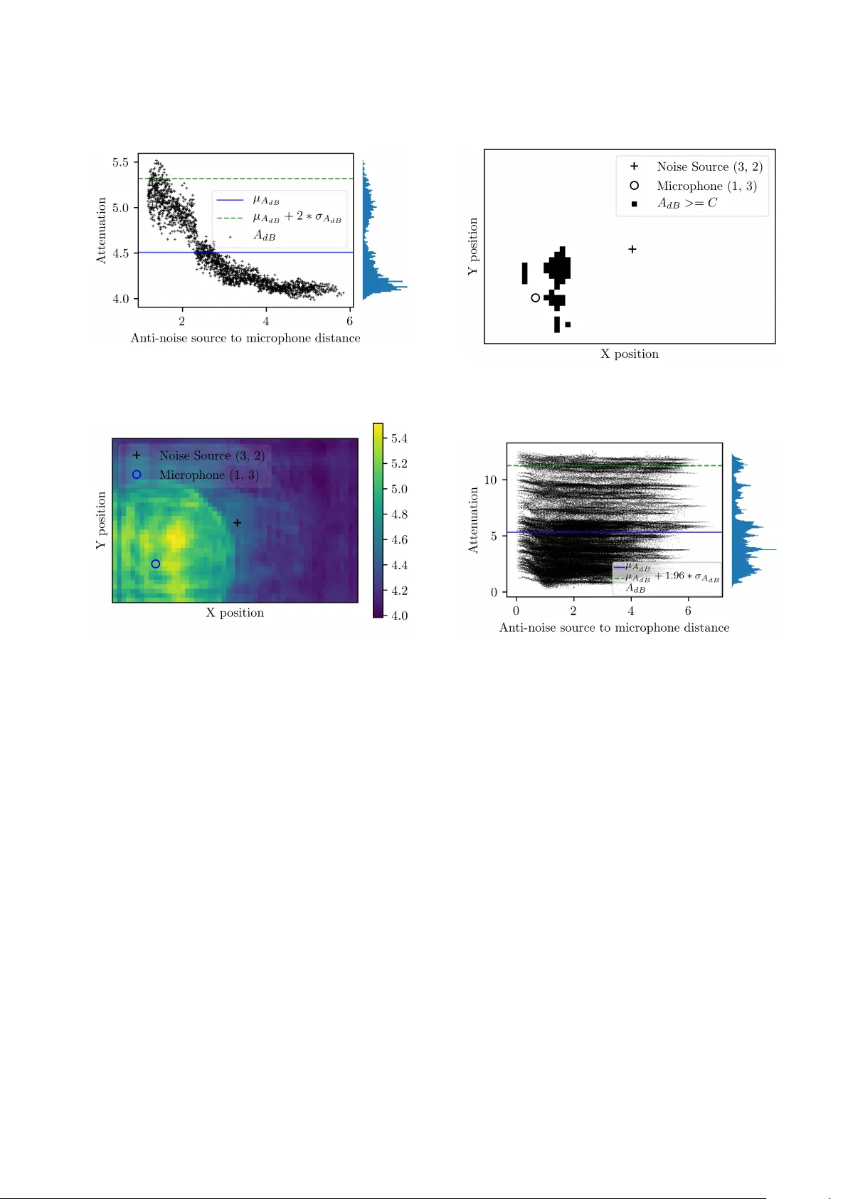
Effect of T ransducer P ositioning in Activ e Noise Contr ol Sajil C. K., Biji C. L and Achuthsankar S. Nair Abstract — Research in traditional Active Noise Con- trol(ANC) often abstracts acoustic channels with band-limited filter coefficients. This is a limitation in exploring structural and positional aspects of ANC. As a solution to this, we propose the use of room acoustic models in ANC resear ch. As a use case, we demonstrate anti-noise source position optimization using room acoustics models in achieving better noise control. Using numerical simulations, we show that le vel of cancellation can be impro ved up to 7.34 dB. All the codes and results are av ailable in the Github repository https://github.com/cksajil/ancram in the spirit of reproducible research. I . I N T RO D U C T I O N Studies hav e prov en that exposure to high sound pressure lev els for extended periods of time can cause temporary or permanent hearing loss [1]. In the medical field, MRI scan- ners generate noise over 120 dB [2], which is often causing discomfort to the patients [3] as well as to doctors. There hav e been studies proving that the noise generated by fMRI scanners affect the scanning results also [4]. One solution to this is acoustic quiet zones generated by Acti ve Noise Control(ANC), which have broad applications in medical, entertainment, automobiles [5], airplanes, recording studios etc [6]. Recently , noise cancellation concepts were found application in synthetic biology also [7]. Passi ve noise control uses b ulky sound absorbent materials to mask unwanted sound, whose performance degrades for low-frequenc y sounds [6]. ANC systems use the principle of canceling the sound wav e with its in verse or anti-noise. The idea made its first appearance in the patent of Paul Lueg [8]. Figure 1 sho ws a graphical description of a simple active noise control system. Compared to passive noise control techniques, ANC techniques are well able to control low as well as high-frequency noise components. Also, it does not require bulky materials, making it portable. In the existing ANC literature, which has a history of 7 decades [9], the acoustic channels are mostly modeled using Finite Impulse Response(FIR) filters [10]. This ap- proximation, used for ease of computation, limits researchers in studying the effects of physical aspects like transducer positioning, orientation, room rev erberation, wall reflections, room structure etc. Positioning of transducers is an im- portant parameter which is to be addressed in ANC [11]. Room Impulse Response(RIR) is analogous to an Impulse Response(IR) in Linear Time in v ariant(L TI) systems. The IR is considered to characterize the behavior of an L TI This w ork was supported by Univ ersity Grants Commission(UGC), New Delhi, India Authors are with Department of Computational Biology and Bioinformatics, Univ ersity of Kerala, K erala, India sajilckdcb@keralauniversity.ac.in Fig. 1. Illustration of active noise control. The microphone receives the signal from the noise source and feeds into a controller . Controller analyses and drives the anti-noise source with phase in verted signal. Both signals cancel each other at the region of interest. system completely . W ith room acoustics models, it is easy to calculate RIRs between any two points. Though some work make use of measured RIRs for simulation and experimental validation [12][13], a large scale utilization of RIRs using room acoustic models in ANC is still an unexplored area. In the subject area of room acoustics, simultaneous multi channel RIRs were used to reconstruct room geometry [14]. Inspired by their work, we focus to explore the use of RIRs in the Activ e Noise Cancellation(ANC) context. Our major contributions are: • The use of room acoustic models in ANC. • A new workflow model for ANC research. • Optimization of anti-noise source location which im- prov es cancellation up to 7.34 dB. Section II introduces the fundamental of ANC concepts. Section III gi ves a brief overvie w of room acoustics mod- els. The simulation details can be found in Section IV. Results are discussed in detail in Section V, including limitations of our approach and future scope. A tuto- rial style treatment of the research work is av ailable at https://cksajil.github .io/ancram/ aiming at a novice reader . I I . A N C P R E L I M I NA R I E S Existing ANC systems use a controller to predict the noise of interest which is to be canceled. The ANC system picks up the noise using single or multiple microphones and passes on to the controller . The acoustic channel from the noise source to the zone of interest is represented using a primary propagation path P ( z ) . Similarly , the acoustic channel from anti-noise source to the zone of interest is represented using a secondary path S ( z ) . The adaptiv e filter keeps on updating its coefficients so that the error signal at the zone of interest is minimized. The weights of the controller filter Fig. 2. Block diagram of FxLMS ANC System. P ( z ) represent the acoustic channel from the noise source to the microphone. Similarly S ( z ) represents the acoustic channel from anti-noise source to the microphone. The adaptive filter is controlled by the LMS algorithm which also considers the estimate of secondary path ˆ S ( z ) forming FxLMS. are updated using adapti ve filter algorithms like Least Mean Square(LMS), Recursive Least-Squares(RLS) or Filtered-x Least Mean Square (FxLMS). Among the several types of ANC algorithms av ailable, we tried our hypothesis with the popular and widely used FxLMS algorithm [15] due to its robustness and ease of computation. Figure 2 sho ws block diagram of a tradi- tional FxLMS-ANC system. The transformation happening to source signal x ( n ) , after passing through the primary propagation path P ( z ) , is modeled using the following equation. d ( n ) = x ( n ) ∗ p ( n ) (1) The ’ ∗ ’ here represents conv olution operation. FxLMS algorithm also uses an estimate of the secondary path ˆ S ( z ) , through which a filtered v ersion of the source signal is calculated and passed on to the LMS filter . ˆ x ( n ) = ˆ s ( n ) ∗ x ( n ) (2) The error signal e ( n ) and the filtered reference signal ˆ x ( n ) are used to update the adaptiv e filter weights. w ( n + 1) = w ( n ) + µe ( n ) ˆ x ( n ) (3) Here, w ( n ) = [ w 0 ( n ) w 1 ( n ) ... w L − 1 ( n )] are the filter weights, L is the filter length and µ is the step size. In an ideal scenario, after several iteration, the predicted signal ˆ d ( n ) reaches in versely equal to d ( n ) and e ( n ) becomes zero. At this stage the filter weights w ( n ) will be at its optimum con verged range. I I I . R O O M A C O US T I C S M O D E L S Scientists working in acoustics or audio signal processing will often require a stage to test out and reproduce algorithms in specific acoustic scenarios. For this purpose, Room Acous- tics Models(RAM) are often used, to recreate and reproduce room acoustics without any cross-model mismatch. Room acoustic models find its applications in beamforming [16], Fig. 3. Room impulse response as a superposition of direct sound and reflections. The direct sound (source S to receiv er R ) is shown with solid arrow and reflections with gray arrows. The reflections of the direct sound appear to the receiv er as coming from imaginary sources S 1 , S 2 , S 3 and S 4 which are scaled and delayed accordingly . acoustic auralisation, speech and audio processing [17], psychoacoustics studies etc [18]. A RIR model channel between a fixed source and a fixed receiv er with direct path and reflections [14]. In RIR, apart from the direct sound, the receiver recei ves signals from different reflections. The acoustic energy gets attenuated after ev ery reflection. A receiv er at any point will be receiving direct sound superimposed with its reflections as rev erberated sound. Image method [19] has been used widely to calculate RIRs for various room conditions. In image source model, the reflections are considered coming from virtual sources. Figure 3 shows a diagrammatic representation of RIR for an arbitrary 2D room. I V . N U M E R I C A L S I M U L A T I O N S E T U P Figure 4 shows the flow diagram of the simulation. The room size was chosen arbitrarily to a size of 6 × 4 × 3 meters. The z lev el of microphone, noise source and anti-noise source were fixed to a height of 1.53 for ease of computation. The x coordinate for noise source and microphone were chosen randomly from a uniform distribution within half- open interval [1 , 6) . Similarly the y coordinate value for microphone and noise source were chosen randomly from a uniform distribution within half-open interv al [1 , 4) . The antinoise source positions were ev enly spaced at a distance of 11 cm . For each position, anti-noise source is placed in that location and the primary path and secondary path, which are acoustic channels from the noise source to error microphone and anti-noise source to error microphone are calculated. The toolbox provided by Habets [20] ha ve been used for generating the RIRs. These RIRs were passed onto the ANC simulation program. A total of 100 independent Monte-Carlo simulations were carried out for different noise source and microphone positions. T able I shows an arbitrary case for illustration purpose. The noise source is fixed at center of room and the receiving microphone is placed arbitrarily at (1 , 3 , 1 . 5) similar to [21]. Figure 5 shows energy decay curves of room impulse responses for the arbitrary case. Fig. 4. Sequential steps in carrying out the simulation. For each anti-noise source location, RIRs were calculated using room acoustics models and passed onto ANC algorithm. The final canceled signal is analyzed and per- formance metrics(estimated attenuation and frequency specific attenuation) are logged for later reference. T ABLE I S I MU L A T I O N S ET T I N GS U SE D F O R A N A R B IT R A RY C AS E No Parameter V alue 1. Room size 6 × 4 × 3 meters 2. Noise source location (3 , 2 , 1 . 5) 3. Receiv er location (1 , 3 , 1 . 5) 4. Refection coefficients [0 . 8 , 0 . 7 , 0 . 6 , 0 . 5 , 0 . 4 , 0 . 5] Fig. 5. Ener gy Decay Curves of Primary Path P ( z ) and Secondary Path S ( z ) for simulation parameters as per T able I The source signal considered is sinusoidal with a wideband component. W e used the same method to generate the source signal as used here [22] except the fact that we used open source scientific computing language Python [23] for signal generation and simulation. The method to generate the noise signal including source code can be found in the abov e reference. Similarly our source codes for the signal generation and simulation is av ailable in the project GitHub repository [24]. The sinusoidal components consists of a fundamental frequency of 30 Hz and 2 other components which are multiples of the base frequency(i.e, 60 and 90 Hz ). The signal is generated using Fourier synthesis method. The coefficients of sine components were, -1, -0.5 and 0.1 and that of cosine components were 2, 1 and 0.5. The Po wer Spectral Density(PSD) of the source signal is shown in Figure 6. Fig. 6. Power Spectral Density of source signal used. The narrow band components can be seen at 30 Hz , 60 Hz and 90 Hz . A wide band component of variance 0.1 has been added to the signal. T ABLE II P A R AM E T E R V A L UE S U S E D F O R S I MU L A T I O N No Parameter V alue 1. Sampling rate 2 kHz 2. Room size 6 × 4 × 3 meters 3. Simulation time 100 seconds 4. Sound speed 343 meters / seconds 5. Rev erberation time 0 . 4 seconds 6. RIR length 1000 samples 7. Microphone type omnidirectional The sampling frequency(Fs) is fixed to 2 kHz according to Nyquist theorem. The adaptiv e filter length was fixed as 350 at Fs = 2 kHz , which is an important parameter determining ANC performance [25]. A step size of 1 × 10 − 5 was chosen since we wanted to focus on the level of cancellation achiev ed rather than how quickly it is achieved. T able II shows major settings and parameter values used for the simulation. The assumptions made in this study are as follows. The room is considered to be rectangular in shape with size 6 × 4 × 3 meters, without any furniture or moving objects. The reflection coefficient of the six walls are assigned equal and are considered to be frequency independent. The sources and receivers are assumed to be with omnidirectional. The algorithm was simulated for a simulation time of 100 sec- onds. The RIRs calculated were truncated to 1000 samples corresponding to its re verberation time(T60). The secondary path transfer function which abstracts away reconstruction filter , power amplifier, loudspeaker , the acoustic channel from anti-noise source to receiver , pre-amplifier , anti-aliasing filter and Digital to Analog Con verter(D A C) [26] is assumed to be known and identified in prior . V . R E S U LT S A N D D I S C U S S I O N The resulting signal is analyzed for determining the lev el of attenuation obtained. The performance measure used for analysis is, Estimated attenuation( A dB ), similar to [22], which is calculated using the following formula. A dB = 10 l og 10 V ar[ d ( n )] V ar[ e ( n )] (4) Fig. 7. Different A dB lev els obtained. The simulation settings were as per T able I. It can be seen that the distribution of attenuation lev els shown on the right is bi-modal. Fig. 8. Attenuation obtained with respect to each anti-noise source position. A region of locations with good attenuation can be seen around the microphone’ s location. The simulation settings were as per T able I Where, V ar[ . ] represents the mathematical operation of statistical variance. Since our signal of interest is of zero mean, this is equi valent to Mean Square Error(MSE) mea- sure. W e consider only the steady state value of error signal, e ( n ) by trimming of f the initial one-third of it. The parameter A dB represents the overall attenuation of the noise signal which is calculated for each of the anti-noise source posi- tions. Figure 7 sho ws different attenuation lev els obtained for different anti-noise source positions as per simulation settings in T able I. The attenuation lev els can be visualized as a 2D image, where each point in the image will be representing the steady state attenuation for anti-noise source at that position. Figure 8 sho ws the attenuation le vels corresponding to dif ferent anti- noise source positions as per simulation settings on T able I. T o determine good attenuation locations, we chose top 2 . 5 percentile attenuation le vels by setting a threshold of C = µ A dB + 1 . 96 × σ A dB , where µ A dB and σ A dB represents statistical mean and standard deviation of A dB values. These attenuation values correspond to specific points in the room where the attenuation is relatively high. The corresponding binary figure is sho wn in the Figure 9. As can be seen from the Figure 9, the best locations Fig. 9. Positions representing relativ ely good attenuation. It can seen that the good anti-noise source positions are located near to error microphone. The simulation parameter values were as per T able I Fig. 10. Attenuation levels obtained for 100 Monte-Carlo simulations. It can be seen that the average attenuation is 5.31 dB and it can be optimized up to 12.65 dB making a difference of 7.34 dB. fall near the error microphone location. W e think this may due to spectral flatness of secondary path. When the anti- noise source gets closer to the receiver , the secondary path transfer function approaches flat frequency response and the cancellation improves. The attenuation levels of all cases are shown in the Figure 10. It can be seen that the attenuation lev els spans in the range [0.17 dB, 12.65 dB] dB, with a mean attenuation of 5.32 dB and 3.02 dB standard deviation. Figure 11 shows the Power Spectral Density(PSD) of the signal before and after cancellation at the optimum anti-noise source position. Our work dif fers from pre vious studies in the literature [27] where they concentrate on finding the optimum number of anti-noise sources. Also our results are similar to and reconfirms the findings shown here [26], where they optimize error microphone location by using spectral flatness of secondary path. Compared to these two studies, our method giv es insight into best possible geometrical location for anti-noise source using room acoustic models. The results show the possibility to optimize the anti-noise source location, provided the noise source and receiver posi- tions are known and the RIRs or room reflections coefficients are av ailable. This method has the potential to push further into better cancellation lev els for ANC systems. In a realistic Fig. 11. Power Spectral Density of d ( n ) and e ( n ) . It can seen from the graph that the individual narrow band components are significantly attenu- ated after the the FxLMS algorithm conver ges to its stable performance. scenario, it is possible to calculate reflection coefficients from readily av ailable charts of sound absorption. Also, it is possible to calculate reflection coefficients from RIRs [28]. In most cases, room dimensions and shapes are available from blueprints or architecture design diagrams. This opens up the possibility to optimize transducer locations according to any user requirement scenario. The major drawbacks to our approach are, measurement of real RIRs are time-consuming and tedious. W e have not considered time varying changes of the acoustic channels. Also the dynamic variation of the error levels, i.e., how quickly the ANC system attenuates noise have also been not studied. W e rather focused on the stable attenuation lev els. The secondary path, which is a very important component in ANC systems is assumed to be kno wn and identified. More accurate RIR models will require lengthy RIRs which contributes to computational complexity . There is a tremendous scope for improvement in our w ork including verifying the results in real lab conditions, improving ease of computation using a more concise representation of RIRs, moving observer or source scenario etc. V I . C O N C L U S I O N W e hav e in vestigated the possibility of using Room Acous- tics Models in ANC scenario. W e particularly focused on optimizing anti-noise source location once the noise source and recei ver are fixed. Results prov e that optimizing anti- noise source location impro ves the le vel of cancellation by approximately 7.34 dB. This opens up the possibility of optimizing se veral other physical parameters including, transducer orientation, room shape, etc., in achieving better noise control. Our results show that room acoustic models are good simulation tool which needs more attention by the ANC community . V I I . A C K N O W L E D G M E N T W e are grateful to Univ ersity Grants Commission(UGC), New Delhi, India for providing necessary funds to do this re- search, W e are grateful to Campus Computing Facility(CCF) and Department of Computational Biology and Bioinformat- ics, University of Kerala, India for extending the necessary facilities to carry out this research work. R E F E R E N C E S [1] C. V . R. Sierra, M. J. V ersluis, J. M. Hoogduin, and H. Duifhuis, “ Acoustic fmri noise: linear time-inv ariant system model, ” IEEE T ransactions on Biomedical Engineering , vol. 55, no. 9, pp. 2115– 2123, 2008. [2] M. E. Ravicz, J. R. Melcher , and N. Y .-S. Kiang, “ Acoustic noise during functional magnetic resonance imaging, ” The Journal of the Acoustical Society of America , vol. 108, no. 4, pp. 1683–1696, 2000. [3] G. Kannan, A. A. Milani, I. M. Panahi, and R. W . Briggs, “ An efficient feedback active noise control algorithm based on reduced-order linear predictiv e modeling of fmri acoustic noise, ” IEEE transactions on Biomedical Engineering , vol. 58, no. 12, pp. 3303–3309, 2011. [4] S. Skouras, M. Gray , H. Critchley , and S. Koelsch, “fmri scanner noise interaction with affecti ve neural processes, ” PloS one , vol. 8, no. 11, p. e80564, 2013. [5] P . N. Samarasinghe, W . Zhang, and T . D. Abhayapala, “Recent advances in activ e noise control inside automobile cabins: T oward quieter cars, ” IEEE Signal Processing Magazine , vol. 33, no. 6, pp. 61–73, 2016. [6] S. M. Kuo and D. R. Morgan, “ Active noise control: a tutorial revie w , ” Pr oceedings of the IEEE , vol. 87, no. 6, pp. 943–973, 1999. [7] C. Zechner , G. Seelig, M. Rullan, and M. Khammash, “Molecular circuits for dynamic noise filtering, ” Pr oceedings of the National Academy of Sciences , vol. 113, no. 17, pp. 4729–4734, 2016. [8] L. Paul, “Process of silencing sound oscillations, ” 1936, uS Patent 2,043,416. [Online]. A vailable: https://www .google.com/ patents/US2043416 [9] N. V . George and G. Panda, “ Advances in active noise control: A survey , with emphasis on recent nonlinear techniques, ” Signal pr ocessing , vol. 93, no. 2, pp. 363–377, 2013. [10] D. V eeravasantarao, S. Ajay , L. Behera et al. , “ Adaptiv e active noise control schemes for headset applications, ” IF AC Pr oceedings V olumes , vol. 41, no. 2, pp. 7550–7555, 2008. [11] Y . Kajikawa, W .-S. Gan, and S. M. Kuo, “Recent advances on activ e noise control: open issues and innovati ve applications, ” APSIP A T ransactions on Signal and Information Processing , vol. 1, 2012. [12] R. M. Reddy , I. M. Panahi, and R. Briggs, “Hybrid fxrls-fxnlms adaptiv e algorithm for active noise control in fmri application, ” IEEE T ransactions on Contr ol Systems T echnology , vol. 19, no. 2, pp. 474– 480, 2011. [13] I. T . Ardekani, J. P . Kaipio, A. Nasiri, H. Sharifzadeh, and W . H. Abdulla, “ A statistical in verse problem approach to online secondary path modeling in active noise control, ” IEEE/A CM T ransactions on Audio, Speech, and Language Processing , vol. 24, no. 1, pp. 54–64, 2016. [14] I. Dokmani ´ c, R. Parhizkar , A. W alther, Y . M. Lu, and M. V etterli, “ Acoustic echoes reveal room shape, ” Pr oceedings of the National Academy of Sciences , vol. 110, no. 30, pp. 12 186–12 191, 2013. [15] D. Morgan, “ An analysis of multiple correlation cancellation loops with a filter in the auxiliary path, ” IEEE T ransactions on Acoustics, Speech, and Signal Processing , vol. 28, no. 4, pp. 454–467, 1980. [16] I. Dokmani ´ c, R. Scheibler , and M. V etterli, “Raking the cocktail party , ” IEEE Journal of Selected T opics in Signal Processing , vol. 9, no. 5, pp. 825–836, 2015. [17] E. De Sena, N. Antonello, M. Moonen, and T . V an W aterschoot, “On the modeling of rectangular geometries in room acoustic simulations, ” IEEE T ransactions on Audio, Speech, and Language Pr ocessing , vol. 23, no. 4, pp. 774–786, 2015. [18] A. W abnitz, N. Epain, C. Jin, and A. V an Schaik, “Room acoustics simulation for multichannel microphone arrays, ” in Pr oceedings of the International Symposium on Room Acoustics , 2010, pp. 1–6. [19] J. B. Allen and D. A. Berkley , “Image method for efficiently simulating small-room acoustics, ” The Journal of the Acoustical Society of America , vol. 65, no. 4, pp. 943–950, 1979. [20] E. A. Habets, “Room impulse response generator, ” T echnische Uni- versiteit Eindhoven, T ech. Rep , vol. 2, no. 2.4, p. 1, 2006. [21] A. Barkefors, M. Sternad, and L.-J. Br ¨ annmark, “Design and analysis of linear quadratic gaussian feedforward controllers for activ e noise control, ” IEEE/ACM T ransactions on Audio, Speech and Language Pr ocessing (T ASLP) , vol. 22, no. 12, pp. 1777–1791, 2014. [22] D. Bismor, “Comments on a new feedforward hybrid anc system, ” IEEE Signal Processing Letters , vol. 21, no. 5, pp. 635–637, 2014. [23] T . E. Oliphant, “Python for scientific computing, ” Computing in Science Engineering , vol. 9, no. 3, pp. 10–20, May 2007. [24] C. K. Sajil. (2017) ancram. [Online]. A vailable: https://github.com/ cksajil/ancram [25] D.-C. Chang and F .-T . Chu, “Feedforward active noise control with a new variable tap-length and step-size filtered-x lms algorithm, ” IEEE/ACM transactions on audio, speech, and language processing , vol. 22, no. 2, pp. 542–555, 2014. [26] S. M. Kuo, S. Mitra, and W .-S. Gan, “ Active noise control system for headphone applications, ” IEEE T ransactions on Control Systems T echnology , vol. 14, no. 2, pp. 331–335, 2006. [27] S. K. Katsikas, D. Tsahalis, D. Manolas, and S. Xanthakis, “ A genetic algorithm for activ e noise control actuator positioning, ” Mechanical Systems and Signal Processing , vol. 9, no. 6, pp. 697 – 705, 1995. [28] E. A. Lehmann and A. M. Johansson, “Prediction of energy decay in room impulse responses simulated with an image-source model, ” The Journal of the Acoustical Society of America , vol. 124, no. 1, pp. 269–277, 2008.