Drift-Free Indoor Navigation Using Simultaneous Localization and Mapping of the Ambient Heterogeneous Magnetic Field

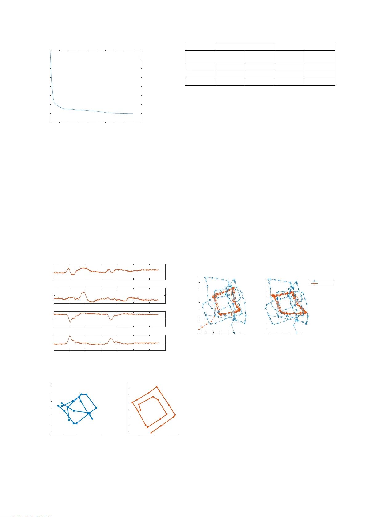
DRIFT - FREE INDOOR NAVIGATION US ING SIMULTANEO US LOCALI ZATION AND MAPPI NG O F T HE AMB I E NT HETEROGENEOU S MAG NETIC F IELD J. C. K. C how Xsens T ec hnologi es , Panthe on 6a, 7521 PR Ens chede , T he Ne therl ands - jacky .cho w @ xsens.com Com m ission IV, W G IV/5 KE Y WO RDS : IMU , M agneto meter , SLAM , Multi - Sensor F usion , I ndoor N av igation ABSTRACT: In the absence of extern al r eference p ositi on informatio n (e.g. surveyed targets o r Global Navigation Satell ite System s ) Sim ulta neous Loc aliz ation a nd Mapping (SL A M) ha s pr ov e n to be a n ef fe ctiv e m et hod for i ndoor nav iga tion. T he posi tioning drif t ca n be re duced with reg ular loop - closure s and global relax ation a s the back end, t hus ac hiev ing a good bal ance betw ee n ex plorat ion and e xploita tion. Alt hough v ision - based system s like laser scanners ar e typically depl oyed for SLAM, th ese senso rs are heavy, energy inefficient , and expensive, making them un attracti ve for wearables or smartpho ne app licatio ns. Ho wever, t he conce pt of SLA M c an be e xte nded to non - opti cal systems such as magn etom ete rs. Inste ad of m atc hing f eat ures s uch a s w alls and f urniture using som e v ari ation of the Iterative Closest P oint algorithm, the local m agnetic f ield can be m atched to provide loop - closur e and g lobal traj ector y updates in a Gaussian P rocess (GP) SLAM framew ork. With a MEMS - based ine rtia l mea sure m ent unit providi ng a c ontinuous t raje ctor y, and the matc hing of locally distinct m agnetic f ield m aps, experim ental re sults in this paper show that a drift - f ree navig ati on solution in a n indoor env ironm ent wi th millim etre - level accuracy can be achieved . The GP - S LAM approach pr esented can be formulat ed as a max imum a posteriori estim ation problem and it can na turall y perf orm loop - detection , feature - to - featu re dist ance minimizatio n, global trajectory optimiz ation, and m ag netic fi eld m ap e stim a tion sim ult aneous ly . Spat ially c ontinuous f ea ture s (i.e . sm ooth magnetic field sign atures) are used instead of discret e feature cor respon dences (e.g. po int - to - point) as in conv entiona l vi sion - based SLA M. T hes e posit ion update s from t he am bie nt m ag netic fie ld al so prov ide enoug h inf orm ati on for c ali brating the ac cel erom et er bias a nd gy ros cope bi as in - us e. The only re stric tion f or this m ethod is the nee d f or m agne tic disturba nce s (w hich i s ty pica lly not a n issue for indoor env ironm ent s); how e ver , no assum pti ons ar e re quired f or the ge nera l m otion of the se nsor (e.g. static peri ods) . 1. INTRODUCTION With the VR/ AR market predict ed to be worth $108 billion by 2021 ( Digi - Capital, 2017) o ne importan t t echnical challen ge is indoor posit ion and ori enta tion tra cki ng. A R in a shopping m all, classroo m, or a vo lume to o large for co st effective depl oyment of cameras can benefit from passive po sitio n trackin g . Furthermore, h ead - tracki ng f or A R/VR in ha rsh env ironm ents or con fined sp aces (e.g. a ircraft cockpit) w here it is diff icult to maintain a camera or th e field of vie w is too restric ted , requ ires a lternate sensor s. MEMS inertial mea surem ent units (IMUs) are get ting sm al ler, cheape r, and m ore ubiqui tous. For exa m ple , the y are f ound in m ost s ma rtphone s, drone s, and wearables these d ays. Al though the y can pr ovide position inf orm a tion, their use is usually limite d to orientation tracking. The reason is that s ma ll inertial errors can result in large positional errors due to the int egr ation pr oces s . Anot her w ay of view ing this is that position upda tes are ver y infor ma tiv e f or i mpr oving the ine rtia l solution. Most com m only , s uch posi tion inf orm ati on is provi ded via extern al s ensors s uch as GNSS, UWB, cameras, sonar, and l asers. RF- based s ystems that prov ide absolut e position upda tes typica lly require additional infras tructure that may not b e availabl e ind oors. Optical systems tha t ca n provide relative position upd ate s are more flexible bu t requir e direct line - of - sight , which me ans the se nsor c annot be placed inside pocke ts or ba gs . Relativ e position upd ates from magnetometers provide a v iable solution t o all t he abov e proble m s. M agne tic s igna ls ha ve be en use d for indoor positioni ng by fing erpr inting tec hniques ( Zhang et a l., 2016 ) (requi res a pre - surv ey ing phas e) and SL A M tec hniques ( does not r equire a pre - surv ey ing pha se ) ( Ferris et al., 200 7 ). In SLA M, the pose is oft en est imated usin g a parti cle filter an d the magneti c map is modelled separatel y ( Vall ivaara et al., 201 1 ) . T he m ethod prese nted i n this pa per c ombi nes t he pose esti ma tion w ith the magnetic map modelli ng in t he Gaussian P ro cess Regress ion (GPR) f ramework. Compare d to popula r Li DA R - based SL AM wor kf low s it has a hig her c om putati on load, but ha s t he advantage t hat many of the key steps are i ntegrated into a single least - squares adjus tm ent to allow tuning param eters to adapt to the dat aset aut omatically. Fo r example, mos t of the m an ually tune d parameters, such as neig hbourhood siz e f or surface modelling, are tra ined by the data . 2. MATHEM ATICAL M ODEL 2.1 Inertial Data Most m oder n day IMU s perform strap - down i nteg ration a t a high f reque ncy (e .g. k ilohe rtz) and the n report odom etr y infor ma tion a s c hange in rota tion ( dq ) and change in velocity ( dv ) at a lo wer , user - desired rate. Given the initial condi tions, the orientation ( q ) , velocity ( v ) , and posi tion ( p ) o f an IMU can be co mputed efficiently using E quation 1. To com pens ate f or the bias es in the accel erometers ( b a ) and g y roscope s ( b ω ) , a random w alk m odel is adopte d ( Equation 2). Note: T is the strap - down integ rati on period, g is the gravity v e ctor, R is the rotati on m atrix , and t he supe rsc ripts L and S represent the lo cal frame and sensor frame, respectively. (1) (2) 2.2 Mag netic D ata A m ap of the ambien t magnetic field strength can be easi ly constr uc ted using spatial interpolation techniq ues (e. g. lin ear or bi - cubic interpolati on) w hen the trajecto ry of the s ensor is known (e. g. measured b y a cam era - based position tracking system ( Solin et al., 2015) ). However, su ch absolut e posit ion informa tion is typically expensiv e or diff icult to obtain. It is mor e com m on to have rela tiv e posit ion inf orm ation i n indoor navigation . Assuming a calibr ated tri - axial ma gnetom eter that is time synchronized with the IMU is availa ble, the relationship between th e observed m agnetic field vector in senso r frame ( s y m ) and the m ag neti c f ield i n the m apping frame ( L m ) can b e expr ess ed using Equat ion 3 , w here x rep resents the l ocatio n at which the magnetic field was sampled an d th e measurement noise ε m is ass um ed to f ollow a G aus sia n distr ibution. It is worth mentioning that any sm all inertial errors may ac cumulate over tim e, resulting in signif icant drifts in the naviga tion solution. (3) Typ ic ally in ma chine l ear ning te xtbook s the GPR s olution is deriv ed f ollow ing the Ba y esi an inference pri ncip les ( Rasmussen and W illia ms , 2006 ) . Beginning w ith Bay es’ rule (Equation 4) , the mar ginal likelihood is integrate d over the unk now n parameters. The b est estim at e of the unk nowns is then deter m ined by m ax im izing Equat ion 5. (4) (5) Alt hough the com putat ional c om plex ity of t his is O(n 3 ) and the mem ory requi rement is O(n 2 ); this is an ef ficie nt GP R form ulation when the objective is to predict the ma gnetic f ield strength at a new location giv en all the training m agnetic measurements at kno wn locat ion s. In the case o f a tightly - coupled I MU and m a gne tom eter SLA M s olution, it is m ore beneficia l to follow the f requentist’s interpretation , where the probabili ty of the prior multiplied by the likelihood is maximized (Eq uation 6 ); this is the max imum a p osteriori estimate o f the trajecto ry and th e magnetic field map. Note: r is the resi duals, C l is the co variance matrix o f the measurements, and the unk now ns ar e (6) The ambien t magnetic fiel ds are assu med to be real izatio ns of a Ga ussia n random pr oces s prior wi th a given co variance matrix (i.e. kern el) K, wh er e K is t yp ica lly chos en to be the s quare d expone ntial kernel (Eq u ation 7). This enfor ces simple sm oothnes s in the local magneti c field. (7) Eve n though thi s is a val id ass um ption, recent research h as show n that f or m ag neti c f ields the thre e dire ctiona l c om ponents are actuall y correlated . Base d on Maxwell’s equati on t he magnetic field can be spl it into the B field and the H f ield; the B field need s to b e divergen ce - free (no sinks) a nd the H f ie ld needs to be c url - fre e (no swirls) ( Wahlst röm et a l., 2013 ) . The curl - free and d ivergence - free kernel s are given in Equ ation 8 . I nstea d of tr eating t h e x, y, an d z magnetic field s as three independe nt sm ooth s urf ace s , their phys ical correla tion is include d to prov ide a more accurate mode l of the local magnetic map , which transl ates int o a more accurat e trajecto ry estimate. (8) 3. RESULTS AND ANALYSIS 3.1 Simulated Datase ts In GP - S LAM the hy per - parameters ch aracterize the ambi ent magnetic field an d are esti mated usin g the data rather than being tuned m anua lly . It c an be val uable to unde rsta nd the im pacts of di ff er ent m ag neti c f ields on the SL A M soluti on through sim ula tion to bett er unde rsta nd the r equir ements for the proposed m e thodolog y . In all sim ulations below, the sensor is ass ume d to be exhibiting transla tional motion only , in a p lane where th e magnetic field i s measured every 25cm, th e odo metry noise is se t to be 0. 5mm (0. 2% of the dis ta nce travelled) with a bias of 5.0m m i n both X and Y di rect ions , σ f is 0.1, and l is 10cm , unles s othe rw ise s tate d. 3.1.1 Effects of va rying σ f : This p arameter describ es the amplitud e of the magneti c signal. For inst ance, σ f is expected to be small when the magnetic fiel d is ho mogen e ous (e.g. outdoors) and large when n ear ferromagnetic material s (e.g. com puter s and m otors ). σ f can also be i nterp reted as th e no ise of the Gaussian Pr ocess con strain t : t he higher t he value, the lo wer the weight of the spatial correlation in the least - squares adjus tment, and vice versa. Four dif f erent cases o f σ f are shown be low w he re GP - SL AM is perf orm ed w ith t he hy per - parameters being fixed to t heir t rue value. From Figure 1 a nd Ta ble 1 it can b e ob served that t he variation of the am bient field must be s uffic iently la r ge rel ative to the s ensor noise, but b ey ond a ce rtain t hres hold, hav ing more ma gne tic dis turba nces does not im prove the accuracy of the SLA M sol ution. -0.8 -0.6 -0.4 -0.2 0 0.2 0.4 0.6 -0.6 -0.4 -0.2 0 0.2 0.4 0.6 -0.6 -0.4 -0.2 0 0.2 0.4 0.6 -0.6 -0.4 -0.2 0 0.2 0.4 0.6 -0.6 -0.4 -0.2 0 0.2 0.4 0.6 -0.6 -0.4 -0.2 0 0.2 0.4 0.6 -0.6 -0.4 -0.2 0 0.2 0.4 0.6 -0.6 -0.4 -0.2 0 0.2 0.4 0.6 Figu re 1 : Estimated trajectory using G P - SLAM w ith diffe rent true σ f . ( Top Left) σ f = 0.001, (Top R ight) σ f = 0.100, (Bottom Left) σ f = 1.000, and (B ottom Rig ht) σ f = 10.00. The c y an das h line s hows the odom et ry only soluti on, the blue s olid l ine indi cates the GP - SLA M sol ution, and t he re d tria ngle s are the ground tr uth. RMSE [m] Max Error [m] Before SLAM 0.066 0.112 Afte r S LAM, σ f = 0.001 0.189 0.318 Afte r S LAM, σ f = 0.100 0.003 0.005 Afte r S LAM, σ f = 1.000 0.004 0.006 Afte r S LAM, σ f = 10.00 0.003 0.005 Table 1 : Error in estimated trajec tory f or v arious σ f 3.1.2 Effects of a wrong σ f : The quality of the e stim ated hype r - parameters has a dir ect impact on th e overall GP - SLAM solution. In this simulation , th e true σ f is 0.1, but the σ f in the GP - SLAM is fix ed to f our dif f ere nt val ues a s show n be low . It appears fro m the resul ts that it is better to overestim ate σ f rather than under est im ating ; this is lik ely because it is better to be conservat ive and p lace less weight o n th e magnetic field position upda tes rather than “over - t rust in g” the magnetic field . -0.8 -0.6 -0.4 -0.2 0 0.2 0.4 0.6 -0.6 -0.4 -0.2 0 0.2 0.4 0.6 -0.8 -0.6 -0.4 -0.2 0 0.2 0.4 0.6 -0.6 -0.4 -0.2 0 0.2 0.4 0.6 -0.6 -0.4 -0.2 0 0.2 0.4 0.6 -0.6 -0.4 -0.2 0 0.2 0.4 0.6 -0.6 -0.4 -0.2 0 0.2 0.4 0.6 -0.6 -0.4 -0.2 0 0.2 0.4 0.6 Figu re 2 : Estima ted trajectory using GP - SLA M w ith the w rong σ f . (To p Left) σ f = 0.001, (Top R ight) σ f = 0.010, (B ottom Le ft ) σ f = 1.000, a nd (Bottom Ri ght) σ f = 10.00. T he c ya n das h line show s the odom e try only sol ution , the blue solid line indicates th e GP - SLA M sol ution, and t he re d tria ngle s are the g round truth. RMSE [m] Max Error [m] Before SLAM 0.066 0.112 Afte r S LAM, σ f = 0.001 0.206 0.346 Afte r S LAM, σ f = 0.010 0.103 0.174 Afte r S LAM, σ f = 1.000 0.004 0.00 6 Afte r S LAM, σ f = 10.00 0.004 0.006 Table 2 : Error in es tim ate d tra jec tory w hen using the w rong σ f 3.1.3 Effects of va rying l : This length parameter deter mines the radius at whic h the m agne tic fie ld sa mpl es s hould be spatial ly correlated . A large l would indica te t hat ev en f ar points would have a n im pact on t he quer y point. A sm all l usually occurs when the lo cal magnetic field is vary ing rapidly ; therefore , only nea rby points a re us ef ul at pr edic ting t he magn e tic field sig nal at the target location. Tw o dif fe rent cases are simulated where the l p arameter is fixed to the true value s of 0.1m a nd 0.4m (Figure 3 and Table 3). Smaller l means a smaller con vergence regio n fo r GP - S LAM but it can yield m ore accur ate results th an a larger l . Furthermore, a better initial trajectory is need ed to ens ure conve rge nce to the global mi nim um. A larger l can represen t a homog en e ous magnetic field; t herefore the accu racy of the GP - SLAM s olution is com prom is ed due to the la ck of unique ness in th e magnetic signat ure. -0.6 -0.4 -0.2 0 0.2 0.4 0.6 -0.6 -0.4 -0.2 0 0.2 0.4 0.6 -0.6 -0.4 -0.2 0 0.2 0.4 0.6 -0.6 -0.4 -0.2 0 0.2 0.4 0.6 Figu re 3 : Estimated trajectory using G P - SLAM w ith diffe rent true l . (Left) l = 0.1m , and ( Rig ht) l = 0.4m . T he c y an das h line show s the odome try only solution, the blue s olid line indica tes th e GP - SLAM s olution, and the r ed tri angl es a re the ground truth. RMSE [m] Max Error [m] Before SLAM 0.066 0.112 Afte r S LAM, l = 0.1m 0.003 0.005 Afte r S LAM, l = 0.4m 0.012 0.021 Table 3 : Error in estimated trajec tory f or various l 3.1.4 Effects of a wrong l : Estim ating the wr ong length para me ter is compa rable to se tting the w rong neig hbourhood search size. In th is case th e magnetic field was simulated usin g l = 0.1 m. In each tri al, l is fix e d to a d iffer en t ( wrong ) value and its effects on the gl obal SLA M soluti on are reported i n Figur e 4 and T able 4. -0.6 -0.4 -0.2 0 0.2 0.4 0.6 -0.6 -0.4 -0.2 0 0.2 0.4 0.6 -0.6 -0.4 -0.2 0 0.2 0.4 0.6 -0.6 -0.4 -0.2 0 0.2 0.4 0.6 -0.6 -0.4 -0.2 0 0.2 0.4 0.6 -0.6 -0.4 -0.2 0 0.2 0.4 0.6 -0.8 -0.6 -0.4 -0.2 0 0.2 0.4 0.6 -0.6 -0.4 -0.2 0 0.2 0.4 0.6 Figu re 4 : Estimated trajec tory using G P - SLA M w ith the wr ong l . (To p Left ) l = 0.005m , (T op Rig ht) l = 0.050m , (Bot tom Le ft) l = 0.150m , and (B ottom Rig ht) l = 0.400m . T he cyan dash l ine show s the odome try only solution, the blue s olid line indica tes th e GP - SLAM s olution, a nd the r ed tria ngle s a re the ground truth. RMSE [m] Max Error [m] Before SLAM 0.066 0.112 Afte r S LAM, l = 0.005m 0.003 0.004 Afte r S LAM, l = 0.05 0m 0.003 0.005 Afte r S LAM, l = 0.150m 0.004 0.006 Afte r S LAM, l = 0.400m 0.127 0.214 Table 4 : Error in es tim ate d tra jec tory w hen using the w rong l Small errors in l do not hav e a sig nifi cant i mpa ct on t he SLA M solution . While GP - SLAM does not appe ar to be hy pers ensit ive to the neighbour hood radius , it is b etter to und erestimate l than to overestim ate ; this is likely be cause it is better to ignor e val uable i nfor ma tion f rom nea r by points rather than to allow spatial ly uncorr elated measurements from a larger neig hbourhood to inf luenc e the query point. 3.1.5 Effect s of vary ing odometry nois e: Like m ost targ e t- less optical SL AM s olutions , GP - S LAM is sensitive to the initial pose. When the initial trajec tory is s ignifica ntly diff er ent fro m t he tru e traject ory , GP - S LAM tends to con verge to a lo cal min i mu m be cause it uses a non linear l east - square s for m ulation. Unlike fr ame - based optica l SLA M m ethods though, e ach magnetometer read ing represen ts the measur ement of a single point, w hich is ins uff i c ient t o esti m ate t he 3D pos ition and 3D orientation. Hence, it relies he avily on the odometry informa tion to lin k temporall y close measurements. A s show n in T able 5 , a smaller od ometry noise means a larger convergen ce region (i.e. l arger biases i n the odo meter can be handled ) . Although a small odometr y noise is a lway s benef icial, b ey ond a ce rtai n thres hold, m ore pr eci se odom etry does not see m t o im prove the s olution signif icantly . RMSE [ m] Max Error [ m] -0.8 -0.6 -0.4 -0.2 0 0.2 0.4 0.6 -0.6 -0.4 -0.2 0 0.2 0.4 0.6 Odom etry noi se = 0.5m m Before SLAM 0.191 0.328 Afte r SLAM 0.012 0.021 -0.8 -0.6 -0.4 -0.2 0 0.2 0.4 0.6 -0.6 -0.4 -0.2 0 0.2 0.4 0.6 Odom etry noi se = 2.5m m Before SLAM 0.196 0.334 Afte r SLAM 0.012 0.024 -0.8 -0.6 -0.4 -0.2 0 0.2 0.4 0.6 -0.6 -0.4 -0.2 0 0.2 0.4 0.6 Odom etry noi se = 5.0m m Before SLAM 0.201 0.338 Afte r SLAM 0.154 0.222 Table 5 : Erro rs in estim ated trajec tory w hen vary ing the odome try noise. The bias in X and Y are se t to 15m m and l is 0.4m . 3.2 Real Dat asets In the f ollow ing ex perim e nts, a MEMS - based IMU from Xsens Te chnolog ies, the MT i - 300 A ttitude and He ading R ef ere nce System was used. 3.2.1 Indoor Envi ronments : Experi m ent 1 In th e first test , the IMU was placed o n a typical office desk with com puter and sma rtphone within its vicinity . It wa s then moved alo ng a r ectangul ar trajecto ry four times with co m plete over lap betw ee n each l oop. Eve n fr om l ooking at the m ag nitude of the m agne tic me asurem ents it is possible to see the si mi larities betw ee n the f our loops (Figure 5) . In this trivia l exam ple, it is possible to pe rf orm loop - closure d etectio n using auto - correlation since the variation in the ma gnetic f ield is as high a s 1.67 a. u. (J ung and M yung , 2015 ). Figu re 5 : Magnit ude o f the measured magneti c signal when looping t he sa me path f our ti me s. To obtain a sensible initial traje ctory , a wea k z ero position update w a s appli ed to c onstra in the I MU posit ion to be w ithin a one metre rad ius sp here. Th e IMU traj ectory before and after GP - SLAM is s hown i n Figur e 6 . Both the horizonta l and vertical accu racies were improved fro m the centimetre - level to millim etre - level af ter 1800 iter ations . The high num be r of iterati ons i s an unde sira ble tr ait of GP - S LAM as th e Lagrangian cost reduction is quite slow af ter ev ery iteration (Figure 7). -0.2 -0.1 0 0.1 0.2 X [m] -0.15 -0.1 -0.05 0 0.05 0.1 0.15 0.2 0.25 Y [m] Trajectory Before GP-SLAM After GP-SLAM -0.1 0 0.1 0.2 Y [m] -0.02 0 0.02 Z [m] Trajectory Figu re 6 : Estimated tr ajector y from repeating a rectan gular p ath four t im es i n a hete roge neous ma gne tic e nvironm e nt. Iteration # 0 200 400 600 800 1000 1200 1400 1600 1800 2000 Lagrangian Cost -1000 -500 0 500 1000 1500 2000 2500 3000 Figu re 7 : The optimization cost function at ev ery iteration Experi m ent 2 In the s econd e xpe rim ent , the IMU w as m ov ed a round in a spiral pattern similar to the sim ulated trajec tory. This test highli ghts one of the s treng ths of GP - S LAM , which is the unn ecessity for perfect o verlap bet we en each p ass of th e same area. U nlike the first experiment , by study ing the m ag neti c signal alo ne it is diff icult to perform loop - closure d etectio n (Figure 8) . A thr eshold f or the aut o- corre lation will need to be set and the possibility of revisiting the s am e position in a diff er ent dir ect ion wi ll nee d to be ha ndled in the logi c ( Jung and Myung , 2015 ). The estimated t rajector y before and after using the m ag netic f ield to pe rf orm GP - S LA M is prov ided in Figu re 9 . The a djustm ent took 797 it era tions to c onve rge a nd the RMSE of the t rajecto ry is reduced from the centi metre - level to millim etre - le ve l. One of the m ain f ac tors tha t c ontribut ed t o the di fference in trajecto ry is the recovered accelerometer an d gyroscope b iases (Table 6 ). 0 200 400 600 800 1000 1200 1400 0.2 0.3 0.4 Mag x [a.u.] 0 200 400 600 800 1000 1200 1400 0 0.1 0.2 Mag y [a.u.] 0 200 400 600 800 1000 1200 1400 -1.1 -1 -0.9 Mag z [a.u.] 0 200 400 600 800 1000 1200 1400 Sample # 0.9 1 1.1 Mag n o r m [a.u.] Figu re 8 : The measured magnetic sign al when movin g the IMU in a sp iral pat tern u nder a h etero geneous magnetic field. -0.1 0 0.1 X [m] -0.15 -0.1 -0.05 0 0.05 0.1 0.15 Y [m] -0.1 0 0.1 X [m] -0.15 -0.1 -0.05 0 0.05 0.1 0.15 Y [m] Figu re 9 : Th e reco nstru cted sp iral tr ajectory. (Left) befo re GP - SLA M in blue and (R ight) af ter GP - SL AM i n orang e . Before GP - S LAM After GP - SLAM Gy r Bias [d eg] Acc Bias [ m/s 2 ] Gy r Bias [d eg] Acc Bias [ m/s 2 ] X 0.0135 - 0.0030 - 0.0509 0.1043 Y 0.0959 0.0020 0.0023 0.0709 Z - 0.0247 0.0255 0.1326 0.0255 Table 6 : The recovered gyroscop e and accelerometer biases in the adj ustm ent Experi m ent 3 The third exper iment was performed o n a special aluminu m table that is free of f erromagnetic material s . In addit ion, n o magnetic obj ects were placed within one metre of the table . T he IMU was moved in a square pattern multiple tim es. W hen study ing the m ag nitude of the m agne tic m ea surem e nts the fie ld appea rs to be fa irly hom ogen e ous. However, when examining the signal in deta il , a rang e of 0.07 a.u. b etween the maximum and m inim um m agnetic read ing can be perceived. Suc h low ma gne tic dis turba nce pos es a chal leng ing s ituati on f or GP - SLAM . In all ot her test cases , it d id not matter if the squared expone ntial ke rnel or curl - free and di vergence - free kernels were appli ed, th e differences i n the t rajector ies were in significa nt. However, in a near - homog en e ous f ield , a more noti ceable impact of the ch osen kernel can be percei ved. Fi gure 10 shows the GP - S LAM solution u sing the two differe nt kernels. In this scenario neith er kernel was able to reco nstr uct a per fect square - shaped trajecto ry. The squar ed expo nenti al kernel resu lted in a highe r m axi mum e rror but prese rv ed the orthog onali ty of a ll edges, whil e the curl - free and d ivergence - free kernel closed all the loops properl y but deform ed the ove rall geom e try of the trajectory into a n arbitrary quadr ilateral . The latter solution mi ght be pref err ed if it is to be c ombi ned w ith othe r opt ical SLA M solution s, becaus e it is mo re con sisten t internally (i.e. all loop s were prop erly detected ). -0.2 -0.15 -0.1 -0.05 0 0.05 0.1 X [m] -0.2 -0.15 -0.1 -0.05 0 0.05 0.1 0.15 Y [m] Trajectory X [m] -0.15 -0.1 -0.05 0 0.05 0.1 Y [m] -0.2 -0.15 -0.1 -0.05 0 0.05 0.1 0.15 Trajectory Before GP-SLAM After GP-SLAM Figu re 10 : The reco vered squ are traject ory und er a near homog ene ous m ag netic fi eld usi ng G P - SLA M. (Left) Using the square d ex ponentia l ke rnel and (Ri ght) c url - f ree and divergen ce - free kernel. Experi m ent 4 The final indoor e xpe rim ent t ook pla ce on a ty pica l w ooden office desk. The MTi - 300 was treated li ke a pen , as it was moved alo ng the surf ac e w riti ng the wor d “X sens”. After GP - SLAM the han dwritten charact er s b ecame legible even tho ugh no acti ve beacon s were intro duced . 0.2 Y [m] -0.2 0 0.2 X [m] -0.2 0 Figu re 11 : Re cove red c om plex handw riting patt ern us ing the ambient magnetic field. (T op) be fore perf orm ing G P - SLAM and (Bottom) after GP - SLA M. 3.2.2 Outdoor E nvironments : In a real homog eneous magnetic field environ ment , GP - S LAM has a fa voura ble pr operty of not m ak ing t he initi al sol ution a ny wor se. T o demons trat e this, the alum ini um t able w a s m ove d outdoors int o an open f ie ld w here t he IMU wa s m ov ed along a rectangu lar track several t imes. I n th is case, th e l of the hy pe r - parameter app roaches a large number rapid ly , σ f app roaches zero, and th e adj ustment con verges. Math ematically it can be see n fr om E quation 7 that as l app roaches infinity all the covarian ce s appr oach σ f (which is zero ), effe ctively disabling all spatial correla tions automatica lly. In conve ntional loo p- closu res in SL AM , a wrong asso ciatio n can h ave a devastati ng effect on the entir e solution due to t he str ong as sum ption be ing m a de in the global relax ation step. In GP - SLAM , the assum pti on being made is much weaker and th erefore has a smaller impact on t he solution w he n the as sum ptions are viola ted ; i.e. it is more robust . -0.1 -0.05 0 0.05 0.1 X [m] -0.1 -0.05 0 0.05 0.1 Y [m] Trajectory Before GP-SLAM After GP-SLAM Figu re 12 : Es timated rectan gular t rajector y pattern in a homog ene ous magnetic field envir onment 4. CONCLUSION AND FUTUR E WO RK This pap er addr esses the probl em of i ndoor nav iga tion by exploiting m agnetic disturbances in a G P - S LAM fr ame wor k with a tightly - coupled M EMS IMU. The orientation, velocity, position, sens or bias es, hy pe r - parameters , and magnetic field map were all e stima ted simultane ously while perf orm ing continuous loop - dete ction a nd loop - clos ure in a b atch least - square s a djustm ent . Through di ff er ent experiments it was shown that magnetic field SLAM in a GPR framework can improve the overall traje ctory w ithout mak ing the solution signific antly w orse. A lthough i t has n o effect on the o verall trajecto ry when appl ied i n ty pical outdoor env ironm ent s, i t can be ar gued that sat ellite si gnals are avail able ou tdo ors an d the magnetometer ca n be used f or he ading update s instead. Future w ork w ill f ocus on im provi ng the efficiency of GP - SLAM through spa rse ke rnel a pproxim a tions in order to scale it to larg er problem s. The curre nt soluti on ass ume s the m agne tic field is not cha nging ; to make it applicable to m ore consum e r appli cation s (e.g. wearabl e tec hnologie s ) the static magneti c map as sumption will be lif ted. ACKNOWLEDGEMENTS This res ear ch is f unded by T RA ck ing i n com plex se nsor systems (TRAX), u nder the EU’ s Seventh Framework Program m e (gra nt ag ree m ent N o. 607400), a nd the N atura l Science and Engin eering Resear ch Council (NSERC) o f Cana da. Valuabl e disc ussi ons w ith Je roen H ol and He nk L uinge are gratefully ackno wledged. REFERENCES Digi - Capital., 2017. Af te r m ixe d y ear , m obile A R to dr ive $108 billion VR/ AR ma rke t by 2021. Ca lif ornia, USA . Ferris, B., Fox, D., & L awrence, N., 2 007 . Wi Fi - SLAM using Gaussian P rocess latent var iable model s. Internati onal Joint Conference on Artificial Intelligence. H yde raba d, India . Jung, J ., & M yung , H., 2015 . Po se - sequen ce - base d gra ph optim iza tion using indoor m a gnet ic f iel d me asurements. In Robot Intell igence Technology and Applic ations 3. A dvance s in Intell igent Sy ste ms and Com puting, v ol 345 (pp. 731 - 739) . Springer, Cham. Rasm ussen, C., & William s, C., 2006 . Ga ussian P rocesses for Machi ne Lear ning. Cam bridge, United States : The M IT P re ss. Solin, A., Kok, M., W ahlstro m , N., Schön, T., & Särkk ä, S., 2015 . Modeling and int erpola tion of the am bie nt m ag neti c f ie ld by G a ussia n proce ss. arXiv prepr int arXi v:1509.04634 . Valli vaara, I., Haverinen , J. , Ke mp p ainen, A., & Röning, J., 2011 . Magnet ic field - based SLA M m et hod for s olvi ng the local iza tion proble m in m obile robot floor - cleanin g task. Inter national Conf ere nce on A dvance d Robotic s. Tallinn, Estonia. Wahlström , N., Kok , M ., Sc hön, T. , & G usta fs son, F., 2013 . Mod eling magnetic f ield s using Gaussian P rocesses. Inter national Conf ere nce on A cousti cs, Spe ec h and Signal Processing . Van couver, Canada. Zhang, M., Shen, W., & Zhu, J., 2016 . WIF I and magneti c fing erpr int posi tioning a lg orithm bas ed on KDA - KNN. Chi nese Control and D ec isio n Conferen ce. Yinchuan, C hina.