Joint Estimation of Room Geometry and Modes with Compressed Sensing

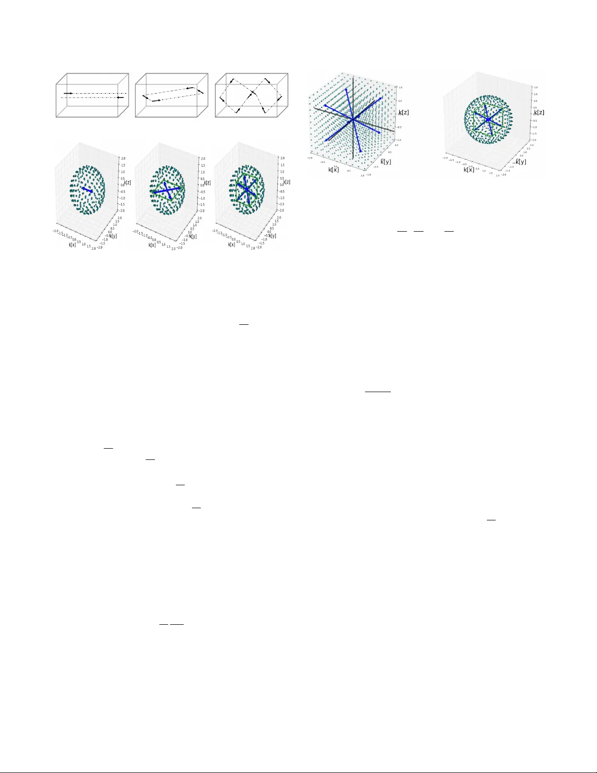
JOINT ESTIMA TION OF THE R OOM GEOMETR Y AND MODES WITH COMPRESSED SENSING Helena P ei ´ c T ukuljac, Thach Pham V u, Herv ´ e Lissek, Pierr e V ander gheynst School of Computer and Communication Sciences Ecole Polytechnique Fed ´ erale de Lausanne (EPFL), CH-1015 Lausanne, Switzerland { helena.peictukuljac, thach.phamvu, herve.lissek, pierre.v andergheynst } @epfl.ch ABSTRA CT Acoustical behavior of a room for a giv en position of micro- phone and sound source is usually described using the room impulse response. If we rely on the standard uniform sam- pling, the estimation of room impulse response for arbitrary positions in the room requires a large number of measure- ments. In order to lower the required sampling rate, some solutions hav e emerged that exploit the sparse representation of the room wa vefield in the terms of plane wa ves in the lo w- frequency domain. The plane wav e representation has a sim- ple form in rectangular rooms. In our solution, we observe the basic axial modes of the wave vector grid for extraction of the room geometry and then we propagate the kno wledge to higher order modes out of the lo w-pass v ersion of the mea- surements. Estimation of the approximate structure of the k - space should lead to the reduction in the terms of number of required measurements and in the increase of the speed of the reconstruction without great losses of quality . Index T erms — compressed sensing, k -space, plane wa ves, room modes, room transfer function 1. INTR ODUCTION In 2006 Ajdler et al. [ 1 ] hav e defined the Plenacoustic func- tion (P AF) as the function that contains the room impulse re- sponses (RIRs) for all the possible pairs of microphone and source positions in a room with the gi ven acoustical proper- ties. W ithout having any prior knowledge in volv ed, it is ex- tremely hard to estimate the P AF . As shown by Moiola et al. [ 2 ] the acoustical behavior of the room can be described by a discrete sum of plane waves that can e xist inside a giv en room which are tightly related to the resonant frequencies. This plane wa ve approximation holds for any star-con vex room and is independent of boundary conditions, domain of prop- agation, type of the source or proximity to the source or the walls [ 3 ]. This work was supported by the Swiss National Science F oundation un- der Grant No. 200021 _ 169360 for the project “Compr essive Sensing applied to the Characterization and the Contr ol of Room Acoustics” . Sparse plane wav e approximation in the low frequenc y domain introduces an assumption required for sparse analysis of room’ s comple x wa vefield which further opens the door to compressed sensing [ 4 , 5 ]. Mignot et al. [ 3 ] ha ve started the trend of the sparse modal analysis. They hav e designed a greedy approach which uses space decomposition based on iterativ e alternating projections for the estimation of the wa ve number and wav e vectors that fully determine the acoustical behaviour of the gi ven room. Due to the high dimensional- ity of data acquired by microphones, greedy methods such as Simultaneous Orthogonal Matching Pursuit (SOMP) [ 6 ] (si- multaneous, since we are fitting measurements from multiple microphones at once) hav e shown better performance than the relaxation of the minimization of ` 0 norm [ 7 ]. Our solution focuses on the structured sparsity of the plane wav e representation for the reconstruction of param- eters of the Room T ransfer Function (R TF). In literature, sparse plane wave representation has been used not only for the representation of the wav efield in a room in low frequency domain, but also for efficient storage of highly correlated recordings of dense microphone arrays [ 8 ]. Besides sparse plane wa ve representation an interesting sparse approach to the estimation of R TF is a recent approach with orthonormal basis functions based on infinite impulse response filters (IIR) [ 9 ]. Though not exploring plane wave sparsity , the solution relying on the weighted spatio-temporal representation [ 10 ] also giv es promising room impulse response interpolations. On the other hand, the solutions for estimating the shape of the room usually rely on knowing the location of early re- flections [ 11 ], [ 12 ], but finding the true reflections within an echogram is not a tri vial problem and is still an open research question. 2. PR OBLEM SETUP When sampling sound we need to tak e into account two types of possible aliasings: temporal and spatial. Depending on the highest frequency that we want to capture f c , we define our temporal sampling step ∆ t in such a way that the sam- pling frequency satisfies f s = 1 ∆ t > 2 f c [ 13 ]. Once the (a) Plane wa ves inside a rectangular room. (b) W a ve v ectors in the search space. Fig. 1 . Plane wav e types and corresponding structured spar- sity of wa ve vectors. In theory these vectors form a paral- lelepiped inscribed into a sphere with radius ω n c , resulting in structured sparsity . From left to right: x -axial mode, xy - tangential mode and oblique mode. temporal sampling step is fixed, we determine the appropri- ate sampling step in space either by the limits imposed by the Courant–Friedrichs–Lewy condition [ 14 ] for finite dif ference time domain (FDTD) schemes, or by a contemporary vie w of the problem observed through the sampling of the P AF [ 1 ]. The support of the spectrum of the P AF ˆ p ( ω , ϕ x , ϕ y , ϕ z ) , where ω = 2 π ∆ t is the temporal angular sampling frequency [ r ad.s − 1 ] and ϕ i = 2 π ∆ i is the spatial angular frequency [ r ad.m − 1 ] over each of the i th observed axis, lays inside a hypercone: ϕ 2 x + ϕ 2 y + ϕ 2 z ≤ ω 2 c 2 , where c is the celerity of sound. This giv es the following condition for the sampling step over each of the axes: ∆ i < π c ω c , ∀ i ∈ { x, y, z } . The following question emerges: can we acquire the targeted in- formation at lower sampling rates, both in time and in space, by exploiting the underlying structure of the data without introducing significant losses? 2.1. Plane wa ve repr esentation of wa vefield Acoustic propagation is gov erned by the wa ve equation: ∆ p ( t, X ) − 1 c 2 ∂ 2 ∂ 2 t p ( t, X ) = 0 . (1) Solution of the wa ve equation can be approximated in the low frequency domain as a discrete sum of damped complex har- monics [ 2 ]: p ( t, X ) = X q ∈ I A q φ q ( X ) g q ( t ) , (2) Fig. 2 . The left hand side shows the periodicity of the wav e vector grid with respect to k = [ ± k x , ± k y , ± k z ] with period ov er the axes equal to: π L x , π L y and π L z . Here we see an e xam- ple of an oblique wav e vector . The right hand side sho ws the search space on our uniformly sampled sphere. where I ⊂ Z , φ q represents the spatial dependency of mode shape whose shape is illustrated in [ 15 ] and g q is correspond- ing time ev olution of the mode. T emporal functions are or- thogonal. This e xpression emphasizes the separability of the analysis and the estimation of the temporal and spatial param- eters, which can greatly reduce the computational complexity of the parameter analysis [ 3 ]. T emporal functions take the form of g q ( t ) = e j k q ct , where k q = ω q − j ξ q c is the wave number of the q th room mode. ω q is the resonant frequency and ξ q < 0 is the corre- sponding damping factor . On the other hand, in the spatial functions, the room modes can be decomposed as a sum of plane wav es: φ q ( X ) ≈ P R r =1 a q ,r e j k q,r · X , where k q ,r is the r th wave vector of the q th mode and R = 8 for a rectangu- lar room case. In Figure 1 . we see an example of all types of plane wa ves in a rectangular room: axial, tangential and oblique determined by the wa ve vectors. In the case of a room with low damping , the length of the wa ve vectors can be approximated by the real part of the corresponding wa venum- ber: k k q ,r k = | k q | , since in that case k q ≈ ω q c . This gi ves us an intuition for the spherical vector search which will be explained more in detail later . For a rectangular room the wa ve vectors are on the vertices of a parallelepiped inscribed into the sphere. Through modal decomposition (3) and plane wa ves approximation, the final form of the RIR is composed of the modal wav e numbers k q ’ s, the corresponding wa ve vectors k q ,r ’ s and their expansion coef ficients α q ’ s: p ( t, X ) = X q ,r α q e j ( k q ct + k q,r · X ) . (3) As in the theory of modal decomposition [ 16 , 2 ], we will focus on the coupling of the pressure field with the standing wa ves at room’ s resonant frequencies. 2.2. Periodicity of the wa ve vector grid In our solution we will be focusing only on the rectangular rooms with the regular wa ve vector grid (regular eigenv alue lattices in the wave vector space) [ 16 ] as shown in Figure 2 . The k-space is an array of numbers representing spatial fre- quencies. According to theory , as long as we know the peri- odicity of the grid o ver each of the ax es, it will provide us the knowledge on the room geometry as well as the values of the wa ve vectors of higher order . So the goal of our approach is the estimation of these three periods along each of the axes. Under the assumptions that the room is lightly damped, the 3 fundamental axial modes can be used as a basis to find all higher order modes. This will reduce the cutoff frequency of the analyzed data, which further reduces the density of the re- quired grid of microphones, due to the dependencies between the temporal and spatial sampling as shown earlier . 3. P ARAMETER ESTIMA TION WITH P AR TIAL COMPRESSED SENSING FOR STR UCTURED D A T A In 1985, Richardson et al. [ 17 ] hav e proposed a curve fitting algorithm allowing the reconstruction of the R TF curve from discrete measurements using room mode shaped functions as basic fitting elements. For different positions of the micro- phones/sound sources across the room, some parameters stay the same - common parameters : eigenfrequencies which de- pend on the room geometry , and the room mode damping which depends on the damping of the walls. The attenua- tion and the phase of the room modes are position dependent parameters - specific parameters which are expressed by dif- ferent expansion coef ficients and different spatial coordinates. 3.1. Acoustical properties of r ectangular rooms There are two key points for our parameter estimation pro- cedure: how many room modes N do we expect up to a giv en cutoff frequency f c and what are their approxi- mate resonant frequencies ω n ? These are dependent on the room shape and size [ 16 ]. For a rectangular room of size L x × L y × L z angular eigenfrequencies are gi ven by the expression: ω n = π c q  n x L x  2 +  n y L y  2 +  n z L z  2 where ( n x , n y , n z ) ∈ N 3 0 \ (0 , 0 , 0) and approximate num- ber of modes up to the cutoff frequency f c is gi ven by: ˜ N f c ≈ 4 π 3 V  f c c  3 where V = L x L y L z . Of special interest will be the basic axial resonant fre- quencies: ω [1 , 0 , 0] = π c L x , ω [0 , 1 , 0] = π c L y and ω [0 , 0 , 1] = π c L z , be- cause they will pro vide the data about the shape of the room. 3.2. Reconstruction procedur e Our goal is to reconstruct spatial periods of the wav e vector grid from low-pass room impulse responses over each of the axes. The size of the room is assumed to be unknown and is Algorithm 1 ReSEMblE algorithm (Algorithm for the joint estimation of Room SizEs and ModEs) Input : A set of measurements { m ( x, y, z , t ) } M i =1 at M known locations X = [ x, y , z ] T in space and T points in time. R ∈ C T × M are measurements in matrix form and r ∈ C T M are measurements in a vectorized form. f p is frequency that separates data into 2 analysis procedures. Output : Estimated room size ˜ L x , ˜ L y , ˜ L z and estimated room transfer function parameters: • expansion coef ficients { α } N ,V n =1 ,v =1 , • resonant frequencies { ω } N n =1 and damping { ξ } N n =1 • wav e vectors { k } N ,V n =1 ,v =1 N : number of modes, V : number of wa ve v ectors per wa ve number . procedur e R E S E M B L E( R , X ) Separate the measurements with f p : R = R l + R h . for i l ∈ { 1 , ..., N l } do step 1 : estimate ( ω i l , ξ i l ) from R l i l step 2 : estimate k i l from r l i l step 3 : compute ne w residual R l i l +1 end for Recov er the room size ˜ L x , ˜ L y , ˜ L z from basic axial room modes and form the regular wa ve vector grid. for i h ∈ { N l + 1 , ..., N } do step 1 : get ω i h and k i h from the wa ve vector grid step 2 : estimate ξ i h from R h i h step 3 : compute ne w residual R h i h +1 end for Estimate the expansion coefficients { α } N ,V n =1 ,v =1 using least square approach. end procedur e jointly estimated. All measured signals are separated into two components: low-pass R l and high-pass R h . Analysis pro- cedure is first applied to the low-pass component, which in- cludes the estimation of the wa ve numbers and correspond- ing wave vectors. The bandwidth of this low-pass analysis is chosen in such a way that it covers reasonable sizes of rooms and remov es the false modes that can appear below the first mode in R TF . W ith f ∈ [20 , 70] Hz we co ver room dimen- sions L x , L y , L z ∈ [2 . 45 , 8 . 575] m for c = 343 m s . This can easily be adjusted for rooms of unusual sizes. 3.2.1. Estimation of ω i l , ξ i l and ξ i h In the low part we define a unit-norm temporal dictionary with atoms of form: Θ[: , i ] = θ [ i ] k θ [ i ] k , where θ [ i ] = e ξ n [ i ] t e j ω n [ i ] t and i is an index on a 2D grid of possible ( ω n , ξ n ) , ω n ∈ [0 , π f s ] and ξ n ∈ [10 ξ 0 , 0 . 1 ξ 0 ] , ξ 0 = − 3 ln 10 RT 60 . The atoms with the highest correlation contains the solution pair . In the high part the frequency is known, so we have only a 1D grid of possible values for the damping, which leads to a much simplified search. 3.2.2. Estimation of k i l The estimation of wav e vectors is done with a structured group sparsity assumption - after estimating the wave num- ber , we construct a sphere with a radius ω n c which follo ws from the assumption of lightly damped modes. W e define a non-unit-norm spatio-temporal dictionary with atoms of form: Σ[: , i ] = e ξ i l t e j ω i l t e X · k [ i ] , where k are samples on this uniformly sampled sphere [ 18 ]. On the surface of this sphere we search for a group of 8 wa ve vectors [ ± k x , ± k y , ± k z ] T which form a parallelepiped and which are aligned with the residual the most. In a case of tangential modes, the parallelepiped collapses over 1 dimen- sion and shrinks to 4 wa ve v ectors (e.g. [ ± k x , ± k y , 0] T ), and axial modes are defined by 2 wa ve vectors (e.g. [ ± k x , 0 , 0] T ). In each iteration the best subgroup of 8 atoms has been es- timated by applying a simultaneous version of matching pur- suit (MP) [ 19 ] and the new residual is estimated by an orthog- onal projection onto the space spanned by the union of all of the subgroups that were previously selected. 4. RESUL TS FOR RECONSTRUCTING THE K-SP A CE OF A RECT ANGULAR R OOM In our solution we ha ve relied on two types of structured spar- sity expected in theory [ 16 ]: wav e vector sparsity as nodes of parallelepiped and wav e vector periodicity in the wa ve vec- tor grid. How does this structured approach af fect the data retriev al? As sho wn in [ 3 , 10 ] efficient interpolation of the sound field is expected only within the part of the room sur - rounded by microphones used for training of the parameters. W e will present the performance of our approach on mea- surements made in a rectangular room with an approximate size 3 m × 5 . 6 m × 3 . 53 m. Properties of the chosen room are observed in [ 20 ]. Microphones are distributed randomly in- side a 1 m side cube in one half of the room and the sound source is in the other half of the room. Since we were pro- cessing real measurements, in order to ha ve an idea about the approximate v alue of some of the parameters we want to esti- mate, we have applied the rational fraction polynomial curve fitting [ 17 ] based on the room mode shaped polynomials as basic fitting elements. This way we have retrie ved approxi- mate resonant frequencies and mode damping factors. Dur- ing the curve fitting process, our wav e numbers k n = ω n + j ξ n c appear in the poles of the fitted function [ 21 ]: p ω ( X ) = ρc 2 ω q P n φ n ( X ) φ n ( X 0 ) K n [2 ξ n ω n + j ( ω 2 − ω 2 n )] . Figure 3 . sho ws the results for the estimation of the room mode resonant frequencies and their position in the k -space in the low part of the algorithm with 20 microphones. Here Fig. 3 . The estimation of wa ve vectors in k -space. The numbers next to the points indicate the corresponding eigen- frequencies (Hz). What we expect from theory in a case with perfectly rigid walls is plotted against the values we get from the measurements. the f p frequency was set to be 70Hz. The basic axial modes are easily recognized and they give a fine approximation of the room size up to a few cm aw ay from ground truth. W e can notice that the k x and k y component of the estimated wav e vectors giv e a good approximation, but there is a slight devi- ation in the k z direction. This is attrib uted to the fact that in the room where the measurements were performed the floor is made from wood and ceiling is made of concrete. Also the slight de viation of the eigenfrequencies can be attributed to the fact that the search of the wav e vectors was performed with a rigid wall model k k q ,r k = | k q | . After applying the high part of the algorithm, the Pearson correlation coef ficient sho wed that the approximation is good (e.g. 82% for only 19-microphone setting and f c = 200Hz ), but it should be further improved once the nature of the de vi- ation of the wa ve vectors is ef ficiently characterized. 5. CONCLUSION The proposed solution is suitable only for rectangular shaped rooms that are lightly damped, which was confirmed by the experiments. Also, the sound source has to be put in a posi- tion such that it excites all the axial modes. Although that the solution requires the N , RT 60 and c parameters to be know , solution is not sensitive to their slight perturbation. The esti- mation of approximate structure of the k -space has lead to the reduction in the terms of number of required measurements and in the increase of the speed of the reconstruction without great losses of quality , but not for a broad range of frequen- cies. The higher we take the frequencies, the greater become the deviations. In the spirit of reproducible research, we hav e decided to open our data and code . 6. REFERENCES [1] T . Ajdler, L. Sbaiz, and M. V etterli, “The plenacoustic function and its sampling, ” IEEE T ransactions on Signal Pr ocessing , vol. 54, no. 10, pp. 3790–3804, Oct 2006. [2] A. Moiola, R. Hiptmair , and I. Perugia, “Plane wa ve approximation of homogeneous helmholtz solutions, ” Zeitschrift f ¨ ur angewandte Mathematik und Physik , vol. 62, no. 5, pp. 809, Jul 2011. [3] R. Mignot, G. Chardon, and L. Daudet, “Lo w fre- quency interpolation of room impulse responses using compressed sensing, ” IEEE/A CM T ransactions on Au- dio, Speech, and Language Pr ocessing , vol. 22, no. 1, pp. 205–216, Jan 2014. [4] D. L. Donoho, “Compressed sensing, ” IEEE T rans. In- formation Theory , vol. 52, no. 4, pp. 1289–1306, 2006. [5] E. J. Candes, J. Romberg, and T . T ao, “Robust un- certainty principles: Exact signal reconstruction from highly incomplete frequenc y information, ” IEEE T rans. Inf. Theor . , v ol. 52, no. 2, pp. 489–509, Feb . 2006. [6] J. A. T ropp, A. C. Gilbert, and M. J. Strauss, “ Algo- rithms for simultaneous sparse approximation: Part i: Greedy pursuit, ” Signal Pr ocess. , vol. 86, no. 3, pp. 572–588, Mar . 2006. [7] J. A. T ropp and S. J. Wright, “Computational methods for sparse solution of linear in verse problems, ” Pr oceed- ings of the IEEE , vol. 98, no. 6, pp. 948–958, June 2010. [8] Y . K oyano, K. Y atabe, Y . Ikeda, and Y . Oikawa, “Physical-model based efficient data representation for many-channel microphone array , ” in 2016 IEEE Inter- national Confer ence on Acoustics, Sp eec h and Signal Pr ocessing (ICASSP) , March 2016, pp. 370–374. [9] G. V airetti, E. De Sena, M. Catrysse, S. H. Jensen, M. Moonen, and T . v an W aterschoot, “ A scalable al- gorithm for physically moti vated and sparse approxima- tion of room impulse responses with orthonormal basis functions, ” IEEE/A CM T ransactions on Audio, Speech, and Language Pr ocessing , vol. 25, no. 7, pp. 1547– 1561, July 2017. [10] N. Antonello, E. De Sena, M. Moonen, P . A. Naylor , and T . van W aterschoot, “Room impulse response inter- polation using a sparse spatio-temporal representation of the sound field, ” IEEE/ACM T ransactions on Audio, Speech, and Language Pr ocessing , vol. 25, no. 10, pp. 1929–1941, Oct 2017. [11] M. Krekovi ´ c, I. Dokmani ´ c, and M. V etterli, “Omnidi- rectional bats, point-to-plane distances, and the price of uniqueness, ” in 2017 IEEE International Confer ence on Acoustics, Speech and Signal Pr ocessing (ICASSP) , March 2017, pp. 3261–3265. [12] Ivan Dokmani ´ c, Reza Parhizkar , Andreas W alther , Y ue M. Lu, and Martin V etterli, “ Acoustic echoes re veal room shape, ” Proceedings of the National Academy of Sciences , vol. 110, no. 30, pp. 12186–12191, 2013. [13] H. Nyquist, “Certain topics in telegraph transmission theory , ” T ransactions of the American Institute of Elec- trical Engineers , vol. 47, no. 2, pp. 617–644, April 1928. [14] H. Lewy , K. Friedrichs, and R. Courant, “ ¨ Uber die partiellen differenzengleichungen der mathematischen physik, ” Mathematische Annalen , vol. 100, pp. 32–74, 1928. [15] H. Pei ´ c Tukuljac, H. Lissek, and P . V anderghe ynst, “Lo- calization of sound sources in a room with one micro- phone, ” SPIE, W avelets and Sparsity XVII , vol. 10394, 2017. [16] H. Kuttruff and E. Mommertz, Room Acoustics , pp. 239–267, Springer Berlin Heidelber g, Berlin, Heidel- berg, 2013. [17] Mark H. Richardson and David L. Formenti, “Global curve fitting of frequenc y response measurements using the rational fraction polynomial method, ” 1985. [18] A. Semechk o, “Suite of functions to per- form uniform sampling of a sphere v 1.3, online, ” https://ch . mathworks . com/ matlabcentral/fileexchange/37004- suite- of- functions- to- perform- uniform- sampling- of- a- sphere , 2015, [Online; accessed 05-October-2017]. [19] S. G. Mallat and Z. Zhang, “Matching pursuits with time-frequency dictionaries, ” T rans. Sig. Proc. , v ol. 41, no. 12, pp. 3397–3415, Dec. 1993. [20] R. Boulandet, J. Mosig, and H. Lissek, T unable Elec- tr oacoustic Resonators Thr ough Active Impedance Con- tr ol of Loudspeakers , EPFL, PhD Thesis, 2012. [21] E. T . J. L. Rivet, Room Modal Equalisation with Elec- tr oacoustic Absorbers , EPFL, PhD Thesis, 2016.