A Graph Signal Processing View on Functional Brain Imaging

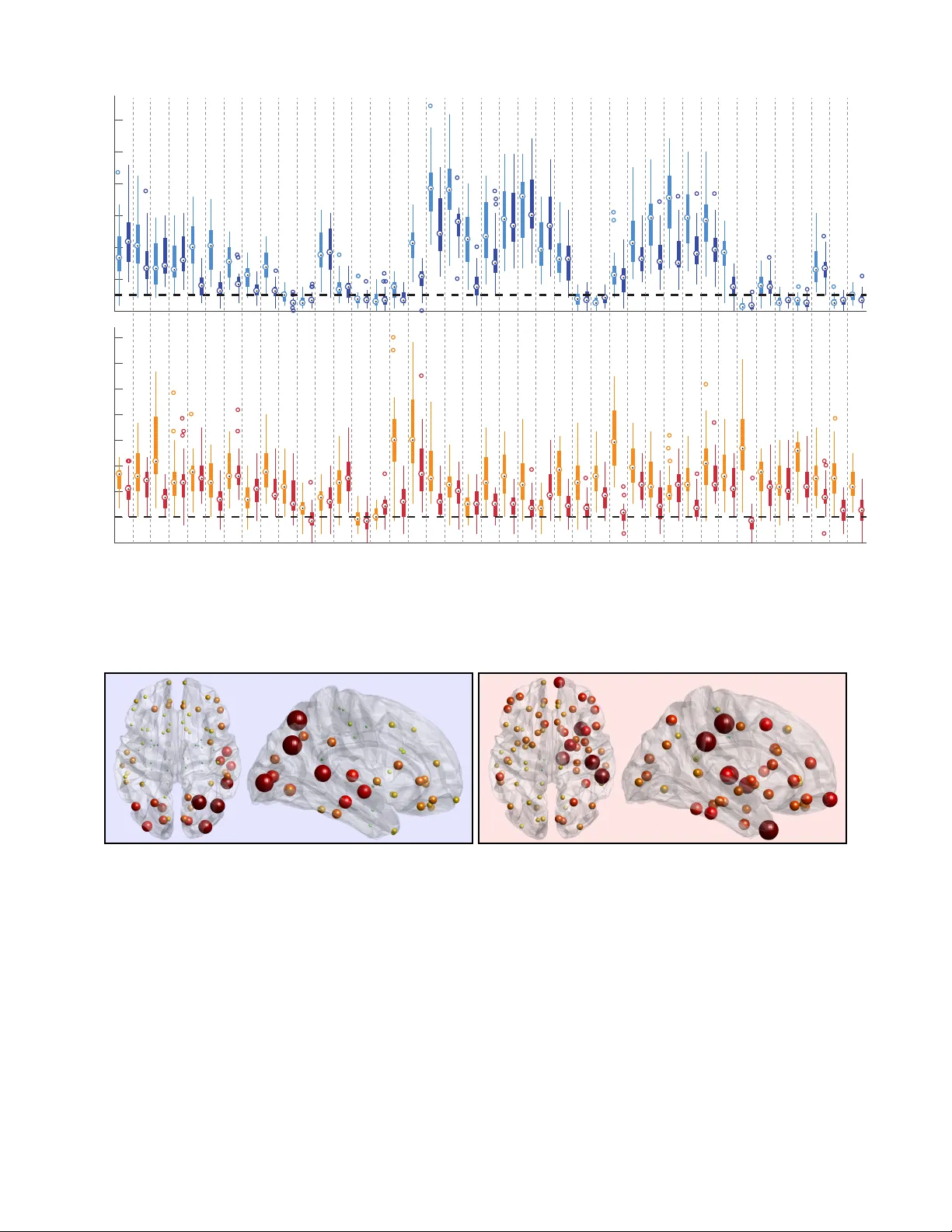
1 A Graph Signal Processing Perspecti v e on Functional Brain Imaging W eiyu Huang ∗ , Thomas A. W . Bolton ∗ , John D. Medaglia, Danielle S. Bassett, Alejandro Ribeiro, Dimitri V an De V ille, Senior Member Abstract —Modern neuroimaging techniques provide us with unique views on brain structure and function; i.e., how the brain is wired, and where and when activity takes place. Data acquired using these techniques can be analyzed in terms of its network structur e to re veal or ganizing principles at the systems level. Graph r epresentations ar e versatile models where nodes are associated to brain regions and edges to structural or functional connections. Structural graphs model neural pathways in white matter that are the anatomical backbone between regions. Func- tional graphs are built based on functional connecti vity , which is a pairwise measur e of statistical interdependency between activity traces of regions. Theref ore, most resear ch to date has focused on analyzing these graphs reﬂecting structure or function. Graph signal processing (GSP) is an emerging area of resear ch where signals recorded at the nodes of the graph are studied atop the underlying graph structure. An increasing number of fundamental operations ha ve been generalized to the graph setting, allowing to analyze the signals from a new viewpoint. Here, we review GSP for brain imaging data and discuss their potential to integrate brain structure, contained in the graph itself, with brain function, residing in the graph signals. W e re view how brain activity can be meaningfully ﬁltered based on concepts of spectral modes derived fr om brain structure. W e also derive other operations such as surrogate data generation or decompositions informed by cognitive systems. In sum, GSP offers a no vel framework for the analysis of brain imaging data. Index T erms —Brain, neuroimaging, network models, graph signal processing, functional MRI I . I N T R O D U C T I O N Copyright (c) 2017 IEEE. Personal use of this material is permitted. Howe ver, permission to use this material for an y other purposes must be obtained from the IEEE by sending a request to pubs-permissions@ieee.org. Supported by ARO W911NF1710438, the Bertarelli Foundation, the Center for Biomedical Imaging (CIBM), NIH DP5-OD021352, the NIDCR R01- DC014960, the Perelman School of Medicine, the John D. and Catherine T . Mac Arthur Foundation, the Alfred P . Sloan Foundation, and the ISI Foundation. The authors indicated with ∗ contributed equally . W eiyu Huang and Alejandro Ribeiro are with the Department of Electrical & System Engineering, Uni versity of Pennsylvania, Philadelphia P A, United States. Thomas A W Bolton and Dimitri V an De V ille are with the Institute of Bioengineering/Center for Neuroprosthetics, ´ Ecole Polytechnique F ´ ed ´ erale de Lausanne (EPFL), Lausanne, Switzerland, and the Department of Radiol- ogy and Medical Informatics, University of Genev a, Geneva, Switzerland. John D. Medaglia is with the Department of Psychology , Drexel Univ er- sity , Philadelphia P A, United States, and the Department of Neurology , Perelman School of Medicine, Univ ersity of Pennsylvania, Philadelphia P A, United States. Danielle S. Bassett is with the Department of Bioengineer- ing and the Department of Electrical & System Engineering, University of Pennsylvania, Philadelphia P A, United States. Corresponding authors: A. Ribeiro (email: aribeiro@seas.upenn.edu) and D. V an De V ille (e-mail: dimitri.vande ville@epﬂ.ch). Some of the results in Section IV are adapted or reproduced with permission from [1]; see [1] for detailed discussion of the implications of these ﬁndings for human cognition. A D V ANCES in neuroimaging techniques such as magnetic resonance imaging (MRI) have provided opportunities to measure human brain structure and function in a non-in vasi ve manner [2]. Diffusion-weighted MRI allows to measure major ﬁber tracts in white matter and thereby map the structural scaffold that supports neural communication. Functional MRI (fMRI) takes an indirect estimate of the brain approximately each second, in the form of blood oxygenation le vel-dependent (BOLD) signals. An emerging theme in computational neu- roimaging is to study the brain at the systems level with such fundamental questions as how it supports coordinated cognition, learning, and consciousness. Shaped by evolut ion, the brain has e volv ed connectivity patterns that often look haphazard yet are crucial in cogniti ve processes. The apparent importance of these connectomes , has motiv ated the emergence of network neuroscience as a clearly deﬁned ﬁeld to study the rele v ance of network structure for cognitiv e function [3]–[5]. The fundamental components in network neuroscience are graph models [6] where nodes are associated to brain regions and edge weights are associated with the strength of the respective connections. This connec- tivity structure can be measured directly by counting ﬁber tracts in diffusion weighted MRI or can be inferred from fMRI BOLD measurements. In the latter case, networks are said to be functional and represent a measure of co-activ ation, e.g., the pairwise Pearson correlation between the activ ation time series of nodes. Functional connectivity networks do not necessarily represent physical connections although it has been observed that there is a strong basis of anatomical support for functional networks [7]. Connectomes, structural and functional alike, hav e been successfully analyzed utilizing a v ariety of tools from graph theory and netw ork science [6]. These analyses have uncov- ered a variety of measures that reﬂect organizational principles of brain networks such as the presence of communities where groups of regions are more strongly connected between each other than with other communities [7], [8]. Network analysis has also been related to behavioral and clinical measures by statistical methods or machine learning tools to study dev elopment, behavior , and ability [9]–[11]. As network neuroscience expands from understanding con- nectomes into understanding how connectomes and functional brain acti vity support beha vior , the study of dynamics has taken center stage. In addition, there is a rise of interest in an- alyzing and understanding dynamics of functional signals and with them, netw ork structure. Such changes happen at dif ferent timescales, from years – e.g., in de velopmental studies [12] – 2 down to seconds within a single fMRI run of se veral min- utes [13], or following tasks such as learning paradigms [1], [11], [14]. So far , common approaches include examining changes in network structure (e.g., reﬂecting segre gation and integration) [15] or in vestigating time-resolved measures of the underlying functional signals [16]–[18]. In the case of dev elopmental studies, the ev olution of structural networks is important, but large-scale anatomical changes do not occur in the shorter time scales that are inv olved in beha vior and ability studies. In the latter case, the notion of a dynamic network itself makes little sense and the more pertinent objects of interest are the dynamic changes in brain activity signals [1], [14]. Inasmuch as brain activity is mediated by physical connections, the underlying network structure must be taken into account when studying these signals. T ools from the emerging ﬁeld of graph signal processing (GSP) are tailored for this purpose. Put simply , GSP addresses the problem of analyzing and ex- tracting information from data deﬁned not in regular domains such as time or space, but on more irregular domains that can be con veniently represented by a graph. The fundamental GSP concepts that we utilize to analyze brain signals are the graph Fourier transform (GFT) and the corresponding notions of graph frequency components and graph ﬁlters. These concepts are generalizations of the Fourier transform, frequency components, and ﬁlters that hav e been used in regular domains such as time and spatial grids [19]–[21]. As such, they permit the decomposition of a graph signal into pieces that represent different levels of v ariability . W e can deﬁne lo w graph frequenc y components representing signals that change slo wly with respect to brain networks, and high graph frequency components representing signals that change swiftly with respect to the connectivity networks. This is crucial because low and high temporal variability have proven to be important in the analysis of neurological disease and be- havior [22], [23]. GFT -based decompositions permit a similar analysis of variability across regions of the brain for a ﬁxed time – a sort of spatial variability measured with respect to the connectivity pattern. W e revie w a recent study [1] that such a decomposition can be used to explain indi vidual cognitiv e differences, as illustrated in Figures 6 and 7, and offer other perspectiv es to apply graph signal processing to functional brain analytics. The theory of GSP has been growing rapidly in recent years, with de velopment in areas including sampling theory [24], [25], stationarity [26], [27] and uncertainty [28]– [31], ﬁltering [32]–[34], directed graphs [35], and dictionary learning [36]. Applications have been spanning many areas including neuroscience [14], [37], imaging [38], [39], medical imaging [40], video [41], online learning [42], and rating prediction [43]–[45]. In this work, we broadly cover ho w GSP can be applied for an elegant and principled analysis of brain activity . In Section II, we start by constructing a graph from structural connectivity—the backbone of the brain—and considering brain activity as graph signals. Then, in Section III, we derive the graph spectral domain by the eigendecomposition of a graph shift operator . Such eigenmodes hav e already been recognized as useful by providing robust representation of the connectome in health and disease [46]. W e introduce a number of graph signal operations that are particularly useful for pro- cessing the activity time courses measured at the nodes of the graph; i.e., ﬁltering in terms of anatomically-aligned or -liberal modes, randomization preserving anatomical smoothness, and localized decompositions that can incorporate additional do- main knowledge. In the following sections, we revie w a recent study in [1] demonstrating the rele v ance of these GSP tools as an integrated framework to consider structure and function: in the conte xt of an attention task, we discuss the potential of GSP operations to capture cognitively rele v ant brain properties (Section IV). W e also pro vide av enues for utilizing GSP tools in the structure-informed study of functional brain dynamics (Section V), through the e xtraction of signiﬁcant excursions in a particular structure/function regime (Section V -A), and by more elaborate uses of GSP building blocks that can broaden the analysis to the temporal frequency domain, or narro w it down to a localized subset of selected regions (Section V -B). As certain parts of the paper include speciﬁc neuroscience terminology , a summarizing table (T able I) is provided for the reader’ s reference. I I . B R A I N G R A P H S A N D B R A I N S I G NA L S Brain networks describe physical connection patterns be- tween brain re gions. These connections are mathematically described by a weighted graph G := ( V , A ) where V = { 1 , 2 , . . . , N } is a set of N nodes associated with speciﬁc brain re gions and A ∈ R N × N + is a weighted adjacency matrix with entries A i,j representing the strength of the physical connection between brain regions i and j . Some readers may prefer to consider the graph as a tuple G = ( V , E ) where E ⊂ V × V describes the existence of physical connections between pairs of brain re gions; each edge ( i, j ) ∈ E has an underlying weight A i,j quantifying the strength of the connection. In this paper , we use G := ( V , A ) because it is more concise; notice that we can infer the existence of an edge ( i, j ) ∈ E from the weight in the adjacency matrix if A i,j > 0 . The brain regions encoded in the nodes of V are macro- scale parcels of the brain that our current understanding of neuroscience deems anatomically or functionally dif ferenti- ated. There are various parcellations in use in the literature that differ mostly in their lev el of resolution [54], [55]. As an example, the networks that we study here consist of N = 82 regions from the Desikan-Killian y anatomical atlas [56] combined with the Harvard-Oxford subcortical parcels [57]. A schematic representation of a few labeled brain regions is shown in Figure 1 (left). The entries A ij of the adjacency matrix A measure the strength of the axonal connection between re gion i and re gion j . This strength is a simple count of the number of streamlines that connect the regions, and can be estimated with diffusion spectrum imaging (DSI) [47] — see Figure 1 for an illustration of the pipeline and Callout 1 for details on the speciﬁc techniques that are used for this purpose. In a situation of healthy development and an absence of trauma, nodes in brain graphs are the same across indi viduals. Inter-subject v ariability of structural connectivity has demonstrated clinical v alue as it 3 T ABLE I N E UR OS C I E NC E T ER M I N OL O G Y U S ED I N T H E PA P ER T erminology Meaning fMRI Measurement of brain activity by detecting changes associated with blood ﬂow BOLD effect When neuronal activity is increased in a brain region, there is an increased amount of cerebral blood ﬂow to the area Connectomes A comprehensive map of neural connections in the brain Nav on switching task A task where participants are asked to switch their attention between global and local features Subcortical system Situated beneath the cerebral cortex Fronto-parietal Implicated in executi ve functions such as cognitive control and working memory , among others Auditory system Responsible for the sense of hearing, and inv olved in linguistic processing Cingulo-opercular Implicated in cognitive control Somatosensory Processes sensations, or external stimuli, from our environment V entral/dorsal attention T ypically reorient attention towards the salient stimuli, and respond with activ ation increases, respectively Default mode In volv ed in processing of one’ s self, thinking about others, remembering the past, and thinking about the future V isual system Enables the ability to process visual detail has been reliably associated with neurological [61], [62] and psychological [63] disorders. Besides structural connecti vity , it is also possible to acquire brain acti vity signals x ∈ R N such that the value of the i th component x i quantiﬁes neuronal activity in brain region i — see Figure 2 for an illustration of these BOLD signals and Callout 2 for details on the methods. BOLD signals for all the N studied brain regions are acquired ov er T successi ve time points, and therefore, we deﬁne the matrix X ∈ R N × T such that its j th column codiﬁes brain acti vity at time j . An example of such a brain signal matrix is provided in Figure 2A, with the corresponding distribution of values for each brain region illustrated in Figure 2B. Brain acti vity signals carry dynamic information that is not only useful for the study of pathology [62], [64], [65], but also enables us to gain insight into human cogniti ve abilities [66]– [68]. Whereas physical connecti vity can be seen as a long-term property of individuals that changes slowly over the course of years, brain activity signals display meaningful ﬂuctuations at second or sub-second time scales that reﬂect how different parts of the brain exchange and process information in the absence of any external stimulus, and how they are recruited to meet emerging cognitive challenges. There is increasing ev- idence that differences in activ ation patterns across individuals tightly relate to behavioral variability [14], [69]–[71]. T o the extent that brain acti vity signals are generated on top of the physical connectivity substrate, brain graphs and brain signals carry complementary information and should be studied in conjunction. This has been a challenge in neuroscience due to the unav ailability of appropriate methods for performing this joint analysis. Here, we adv ocate for the use of GSP tools, as detailed in the following section. I I I . G R A P H S I G NA L P R O C E S S I N G F O R N E U RO I M AG I N G The GSP perspective is to interpret the brain signal x as a graph signal that is supported on the brain graph G = ( V , A ) . Here, we introduce the fundamental operations that we will need for processing neuroimaging data in a meaningful way . A. Graph F ourier T ransform The focus of GSP is not on analyzing the brain graph G per se , but on using that graph to analyze brain signals x . For a graph with positiv e edge weights, we consider a graph shift operator that captures the connectivity pattern of G ; we can choose the adjacency matrix A [19], [20] or the graph Laplacian L = D − A [21], [72], where the degree matrix D contains the degree of each node on its diagonal: D i,i = P j ∈V A i,j . There are also several variants of the graph Laplacian [73] such as the symmetric normalized graph Laplacian L sym = D − 1 / 2 LD − 1 / 2 that factors out differences in degree and is thus only reﬂecting relati ve connectivity , or the random-walk normalized graph Laplacian: L rw = D − 1 L . Generalizations of the graph Laplacian also exist for graphs with negati ve weights [45], [74]. Let us denote the graph shift operator as S and assume henceforth that S is diagonalizable using singular value de- composition or Jordan decomposition, so that S = V ΛV − 1 where Λ is a diagonal matrix containing the eigen values λ k ∈ C , k = 0 , . . . , N − 1 , and V = [ v 0 , v 1 , . . . , v N − 1 ] . When S is symmetric, we hav e that V is real and unitary , which implies V − 1 = V > . The intuition behind examining S as an operator is to represent a transformation that characterizes exchanges between neighboring nodes. The eigendecomposition of S is then used to deﬁne the graph spectral domain. Deﬁnition 1 Consider a signal x ∈ R N and a graph shift operator S = V ΛV − 1 ∈ R N × N . Then, the vectors ˜ x = V > x and x = V ˜ x (1) form a Graph F ourier T ransform (GFT) pair [19], [21]. The GFT encodes the notion of v ariability for graph signals akin to the one that the Fourier transform encodes for temporal signals. When choosing the adjacency matrix A as a shift operator for directed graphs [19], [20], [75], the eigenv al- ues λ k can be complex; the smaller the distance between λ k and | λ max ( S ) | in the complex spectrum, the lower the frequency it represents. This idea is based on deﬁning the total variation of a graph signal x as k x − Sx /λ max ( S ) k 1 , with smoothness being associated to small values of total variation. Then, giv en a ( λ k , v k ) pair , one has total variation with k 1 − λ k /λ max ( S ) k 1 k v k k 1 , which provides an intuitive way to order the dif ferent frequencies. Graph frequency ordering becomes more obvious for undirected graphs and thus symmetric adjacency matrices, as eigen values become 4 C A L L O U T 1 : E S T I M A T I N G B R A I N G R A P H S . MRI allows the acquisition of detailed structural information about the brain. The brain graph inv estigated in the present article was acquired on a Siemens 3.0T Tim T rio with a T1-weighted anatomical scan. T wenty-eight healthy individuals volunteered for the experiment. W e followed a parallel strategy for data acquisition and construction of streamline adjacency matrices as in [47]. First, DSI scans sampled 257 directions using a Q5 half-shell acquisition scheme with a maximum b -value of 5,000 and an isotropic vox el size of 2.4 mm. W e utilized an axial acquisition with repetition time (TR) = 5 s, echo time (TE)= 138 ms, 52 slices, ﬁeld of view (FoV) (231, 231, 125 mm). W e acquired a three-dimensional SPGR T1 volume (TE = minimal full; ﬂip angle = 15 degrees; FO V = 24 cm) for anatomical reconstruction. Second, diffusion spectrum imaging (DSI) was performed to establish structural connectivity . DSI data were reconstructed in DSI Studio using q -space diffeomorphic reconstruction (QSDR) [48]. QSDR computes the quantitative anisotropy in each voxel, which is used to warp the brain to a template QA volume in Montreal Neurological Institute (MNI) space. Then, spin density functions were again reconstructed with a mean diffusion distance of 1.25 mm using three ﬁber orientations per vox el. Fiber tracking was performed in DSI studio with an angular cutoff of 35 ◦ , step size of 1.0 mm, minimum length of 10 mm, spin density function smoothing of 0.0, maximum length of 400 mm, and a QA threshold determined by dif fusion-weighted imaging (DWI) signal in the colony-stimulating factor . Deterministic ﬁber tracking using a modiﬁed F ACT algorithm was performed until 1,000,000 streamlines were reconstructed for each individual. Third, each anatomical scan was segmented using FreeSurfer [49], and parcellated using the connectome mapping toolkit [50]. A parcellation scheme including N = 87 regions was registered to the B0 volume from each subject’ s DSI data. The B0 to MNI voxel mapping produced via QSDR was used to map region labels from nati ve space to MNI coordinates. T o extend region labels through the grey-white matter interface, the atlas was dilated by 4mm [51]. W e used FSL to nonlinearly register the individual T1 scans to MNI space. By combining parcellation and streamline information, we constructed subject-speciﬁc structural connecti vity matrices, whose elements represent the number of streamlines connecting two dif ferent regions [52], divided by the sum of their volumes [53]. This process yields the weighted adjacency matrix A ∈ R N × N for each individual considered here. Brain atlas T ractography Brain graph Fig. 1. Estimating brain graphs . Knowledge from an anatomical atlas based on anatomical features such as gyri and sulci (left) is combined with MRI structural connectivity extracted from diffusion-weighted MRI (middle), which can then be used to estimate the brain graph (right). [Adapted from [53]]. real numbers. Speciﬁcally , the quadratic form of A is gi ven by λ k = v > k Av k = P i 6 = j A i,j [ v k ] i [ v k ] j . In this setting, lower frequencies will be associated to larger eigen v alues, to represent the fact that highly connected nodes in the graph possess signals with the same sign and similar values. When using the graph Laplacian L as a shift operator [21] for an undirected graph, the quadratic form of L is gi ven by λ k = v > k Lv k = P i 6 = j A i,j ([ v k ] i − [ v k ] j ) 2 . If the signal variations follow the graph structure, the resulting v alue will be low . Thus, in this setup, the eigenv ectors associated to smaller eigen values can be re garded as the graph lower frequencies. Further , the basis V is then a common solution to sev eral well known signal processing problems, including Laplacian embedding, where the aim is to ﬁnd a mapping of the graph nodes on a line so that connected nodes stay as close as possible, or in other words, to minimize x > Lx under the constraints x > x = 1 and x > 1 = 0 [76]. Another is the classical graph cut problem [77], [78], where the goal is to partition a graph into sub-communities of nodes with as few cross-connections as possible, with a similar obtained solution upon relaxation of the x i = ± 1 constraint. Besides a decomposition along the spatial domain, we can also use the classical discrete Fourier transform (DFT) to decompose X along its temporal dimension as: ˆ X = XF H , (2) where · H indicates the Hermitian transpose, and F is the Fourier matrix. ˆ X ∈ C N × T contains T Fourier coefﬁcients for each of the N time courses. Filtering can then be applied by multiplying with a diagonal matrix H deﬁned by the windowing function [ H ] i,i = h ( λ i ) , with the ﬁltered output giv en by: Y H = XF H HF . (3) Notice that the DFT can also be obtained using the graph formalism by considering cycle graphs that represent discrete periodic signals [20], [21], [24], [79]. Speciﬁcally , we consider the undirected graph G with adjacency matrix A cycle such that [ A cycle ] i,i +1 mo d T = [ A cycle ] i,i − 1 mo d T = 1 , and [ A cycle ] i,j = 0 otherwise. F or this graph, the eigenv ectors of its adjacency A cycle or its Laplacian matrix L cycle = 2 I − A cycle satisfy V = F . Since cycle graphs are representations of 5 C A L L O U T 2 : E S T I M A T I N G B R A I N S I G NA L S . T o derive the studied brain activity signals, functional MRI (fMRI) runs were acquired during the same scanning sessions as the DSI data on a 3.0T Siemens Tim T rio whole-body scanner with a whole-head elliptical coil by means of a single-shot gradient-echo T2* (TR = 1500 ms; TE = 30 ms; ﬂip angle = 60 ◦ ; FO V = 19.2 cm, resolution 3mm x 3mm x 3mm). Preprocessing was performed using FEA T [58], and included skull-stripping with BET [59] to remove non-brain material, motion correction with MCFLIR T [58], slice timing correction (interleaved), spatial smoothing with a 6mm 3D Gaussian kernel, and high-pass temporal ﬁltering to reduce low- frequency artifacts. W e also performed EPI unwrapping with ﬁeldmaps in order to improve subject registration to standard space. Native image transformation to a standard template was completed using FSL ’ s afﬁne registration tool, FLIR T [58]. Subject-speciﬁc functional images were co-registered to their corresponding high-resolution anatomical images via a Boundary Based Registration technique [60] and were then registered to the standard MNI-152 structural template via a 12-parameter linear transformation. Finally , we extracted region-a veraged BOLD signals using the same atlas as for the structural analysis. At the end of this pipeline, we are thus left with a signal matrix X ∈ R N × T for each subject, reﬂecting the activity levels of all brain regions ov er time. 30 60 90 120 150 0 180 Time [s] Brain regions -100 -50 0 50 100 Brain regions BOLD signal [a.u.] A B -80 80 0 BOLD signal [a.u.] Fig. 2. Example brain activity signals . ( A ) F or an e xample subject, the heat map of BOLD magnitude acti vity across brain regions (v ertically) and time points (horizontally). Brain activity signals can be considered as a two-dimensional matrix, index ed in both the temporal and spatial domains. From the temporal perspective, there are certain time instances (e.g., in this case, between 30 and 40 seconds and between 70 and 80 seconds) when BOLD magnitudes are in general stronger than for others. From the spatial perspective, signals on most brain re gions change in the same direction, b ut there are certain brain regions where their changes do not follow the main trend. As we will see, lo w and high graph frequency components, respectiv ely , can be used to e xtract these tw o different pieces of information. ( B ) For the same subject, distrib ution of fMRI BOLD values for each brain region (horizontally) across all time points. Different brain regions exhibit different levels of variability , b ut in general, the wide variance of BOLD signals complicates data analysis. For each brain region, edges of the box denote 25th and 75th percentiles respectiv ely; whiskers extend to the extreme points not considered to be outliers; circles denote outliers, which are values beyond 1.5 times the interquartile range away from the edges of the box. discrete periodic signals, it follows that the GFT of a time signal is equi valent to the con ventional discrete Fourier trans- form. In other words, a GFT is equiv alent to a DFT for c yclic graphs. W e also note that it is possible to combine DFT and GFT to inv estigate the joint spatial-temporal frequency , i.e., ˆ ˜ X = V > XF H . Such analytical efforts have been developing recently; see [26], [80]–[82] for more details. B. Graph Signal F iltering Giv en the abov e relationships, it becomes possible to ma- nipulate the graph signals stored in the matrix X by extracting signal components associated to different graph frequency ranges. Speciﬁcally , we can deﬁne the diagonal ﬁltering matrix G , where [ G ] i,i = g ( λ i ) is the frequency response for the graph frequency associated with eigen v alue λ i , and retriev e the ﬁltered signals as: Y G = V GV > X . (4) Generic ﬁltering operations can now be deﬁned for the graph setting, such as ideal low-pass ﬁltering, where g ( λ i ) would be 1 for λ i corresponding to lo w-frequency modes, and 0 otherwise. Using the deﬁnition of the GFT pair , the effect of the ﬁltering in (4) on the graph spectral coefﬁcients is directly visible from ˜ Y G = G ˜ X . This also allo ws to generalize the con volution operation of a graph signal x by a ﬁlter deﬁned through the spectral window g as [21]: [ y G ] k 0 = N − 1 X k =0 [ v k ] k 0 g ( λ k ) ˜ x k . It is also possible to translate the operation to the vertex do- main by considering the T aylor approximation of the window function g ( λ ) = P M m =0 c m λ m : Y G = M X m =0 c m S m X , which uses iterated versions of the shift operator S . Other operations such as translation, modulation, or dilation can be generalized in a similar way [21]. C. Generation of Graph Surr ogate Signals A piv otal aspect in an y research ﬁeld is to assess the sig- niﬁcance of obtained results through statistical testing. More precisely , one aims to in v alidate the null hypothesis , which ex- presses the absence of the effect of interest. Standard paramet- ric tests such as the well-known t -test assume independent and identically distributed Gaussian noise, which makes a weak null hypothesis for most applications. Non-parametric tests such as the permutation test provide a powerful alternati ve by mimicking the distrib ution of the empirical data. F or correlated data, the Fourier phase-randomization procedure [83] has 6 Functional data Graph Fourier transform T ransformed functional data Spectral domain Adjacency spectrum low-frequency modes high-frequency modes low-frequency modes Adjacency spectrum Adjacency spectrum high-frequency modes Eigenvalue Regions Regions time BOLD Region 1 Region 2 … BOLD Time Amplitude Mode 1 Mode 2 … Am p l i t u d e Laplacian spectrum Structural connectivity A D B C E 0 Fig. 3. Graph signal processing for brain imaging . ( A ) Structural connectivity from diffusion-weighted MRI, as seen in the form of a sagittal brain view (top) or of an adjacency matrix where the weights represent the strength of the structural connections (bottom), is used to b uild a graph representing the brain’ s wiring scaffold. ( B ) Through the eigendecomposition of the Laplacian (left plot) or adjacency (right plot) matrix, this structural graph can be analyzed in the spectral domain. The smallest Laplacian eigenv alues (or most positiv e adjacency eigenv alues) (labeled in blue) are associated with low-frequency modes on the graph ( C , top brain views), while the largest Laplacian eigen values (or most negativ e adjacency eigen values) (labeled in red) are associated with high-frequency modes ( C , bottom brain views). T ogether , these modes deﬁne the graph Fourier transform. Functional MRI data measured at the nodes of the graph ( D ) can be decomposed using these modes, and transformed by means of graph signal processing tools ( E ). been widely applied as it preserves temporal autocorrelation structure under stationarity assumptions. This standard method can be applied to the temporal dimension of our graph signals: Y = XF H Φ time F , where the diagonal of Φ time contains random phase factors ac- cording to the windowing function Φ( λ l ) = exp( j 2 π φ l ) , with φ l realizations 1 of a random variable uniformly distributed in the interval [0 , 1] . From the surrogate signals, one can then compute a test statistic and establish its distrib ution under the null hypothesis by repeating the randomization procedure; i.e., the power spectrum density of the surrogate data is dictated by the empirical data. Note that in this setting, the spatial features of null realizations are identical to the ones of the actual data, while temporal non-stationary effects are destroyed. The phase randomization procedure can be generalized to the graph setting [84] by considering the GFT . In particular , the graph signal can be decomposed on the GFT basis and then, the graph spectral coefﬁcients can be randomized by ﬂipping their signs. Assuming that the random sign ﬂips are stored on 1 In practice, some additional constraints are added such as preservation of Hermitian symmetry . the diagonal of Φ graph , we can formally write the procedure as: Y = VΦ graph V > X . (5) This procedure generates surrogate graph signals in which the smoothness as measured on the graph is maintained, b ut in which the non-stationary spatial effects is destroyed. The temporal properties of null realizations are identical to those observed in the actual data. D. W avelets and Slepians on the Graph The wav elet transform is another fundamental tool of sig- nal processing [85] providing localized, multiscale decom- positions. Sev eral designs have been proposed to generalize this concept to graphs, such as approaches in the vertex domain [86]–[88], based on diffusion processes [89], [90], or using the spectral domain [79], [91], [92]. The latter design builds upon the GFT and has been applied for multiscale community mining [93] or to in vestigate uncertainty princi- ples [28]–[31]. Here, we detail a more recent design of a localized decom- position for graph signals that is based on a generalization 7 of Slepian functions [94] and that can deal with additional domain knowledge. Let us consider the problem of retrieving a signal x ∈ R N that is maximally concentrated within a subset of nodes from the graph at hand, while at the same time setting a maximal bandwidth on the solution. As the global concentration of a signal is giv en by x > x , we end up maximizing µ = ˜ x > ¯ V > M ¯ V ˜ x ˜ x > ˜ x , (6) where M is the diagonal selectivity matrix with elements M i,i = 0 or 1 to respectiv ely exclude, or include, a node into the sub-graph of interest, and ¯ V ∈ R N × M is a trimmed GFT matrix where only low-frequenc y basis vectors are kept. The interpretation here is that we aim at ﬁnding the linear com- bination of band-limited graph spectral coef ﬁcients enabling the best localization of the signal within the sub-graph. Note that the sub-graph is selected using prior information, and not optimized over . If we deﬁne the concentration matrix as C = ¯ V > M ¯ V , then the problem amounts to solving its eigendecomposition, and { ˜ s k } , k = 0 , 1 , . . . , M − 1 , are the weighting coefﬁcients obtained as solutions. W e assume that the y are ordered in decreasing eigen value amplitude ( µ 0 > µ 1 > . . . > µ M − 1 ), so that ˜ s 0 is the optimal (maximally concentrated) solution. From the set of coef ﬁcients, the Slepian matrix can then be retriev ed as: S = ¯ V ˜ S , (7) where S ∈ R N × M and each column contains one of the Slepian vectors s k . Slepian vectors are not only orthonormal within the whole set of nodes ( s > k s l = δ k − l ), but also orthogonal over the chosen subset ( s > k Ms l = µ k δ k − l ). Now , in order to make Slepian vectors more amenable to the application of GSP tools, let us consider an alternative optimization criterion in which the modiﬁed concentration matrix is given as C 2 = ¯ Λ 1 / 2 C ¯ Λ 1 / 2 , with ¯ Λ ∈ R M × M the trimmed diagonal matrix of eigen v alues. The ne w quantity to optimize then reads: ξ = ˜ x > ¯ Λ 1 / 2 ¯ V > M ¯ V ¯ Λ 1 / 2 ˜ x ˜ x > ˜ x . (8) The set of solution Slepian vectors are still orthonormal, but this time, they satisfy s > k Ms l = ξ k δ k − l . Observe that, when using the Laplacian matrix as our graph shift operator , if all nodes are selected as the subset of interest ( M = I ) while enabling a full bandwidth ( ¯ Λ = Λ , ¯ V = V ), then we fall back on the classical Laplacian embedding case discussed in Section III-A, and as such, this modiﬁed criterion can be seen as a generalization of Laplacian embedding (i.e., a modiﬁed embedded distance criterion) under user-deﬁned bandwidth and selectivity constraints. Analogously to the GFT setting, solution Slepian vectors of increasing eigen v alue ξ k can then be regarded as building blocks of increasing graph frequency , but within the cho- sen sub-graph, i.e., of increasing localized frequency . The conceptual difference between both optimization schemes is illustrated in an e xample dataset of leopard mesh in Figure 4, where the sub-graph is the head of the leopard as sho wn in λ=0.063 μ=0.000 ξ=0.000 λ=0.108 μ=0.288 ξ=0.011 λ=0.192 μ=0.967 ξ=0.183 λ=0.267 μ=0.983 ξ=0.262 A C B 200 400 600 800 1000 0 0.2 0.4 0.6 0 index Embedded distance 0 200 400 600 800 1000 0 0.2 0.4 0.6 0.8 1 index Energy concentration 200 400 600 800 1000 index 0 0.2 0.4 0.6 0 Modified embedded distance Fig. 4. Illustration of Slepian vectors and their properties . ( A ) Within the considered graph (a leopard mesh), the head is selected as the subset of nodes of interest. ( B ) Example Slepian vectors obtained from the modiﬁed embedded distance optimization criterion (8). In each case, alongside localized frequency ( ξ ), embedded distance ( λ ), and energy concentration ( µ ) are also shown. ( C ) For a bandwidth M = 1000 and Laplacian embedding (left), energy concentration (middle) or modiﬁed embedded distance (right) optimizations, sorting of the obtained eigenv alues (respectively λ , µ or ξ ). Figure 4A. Four of the Slepian v ectors derived from (8) are shown with their localized frequency ξ , their energy concen- tration µ computed from (6), and their embedded distance λ = s > Ls . The leftmost example denotes a low frequency on the whole graph, with very weak signal within the selected sub-graph, and thus both low localized frequency and energy concentration. The second Slepian vector shows fairly uniform negati ve signal within the sub-graph, resulting in a quite large energy concentration, but a very low localized frequency . The last two examples reﬂect Slepian vectors that are both strongly concentrated (high µ ) and of high localized frequency (high ξ ). If Laplacian embedding is performed on the full graph (Figure 4C, left plot), the resulting eigen vectors linearly span the graph frequency spectrum (black line). If the energy concentration criterion is used for generating Slepian vectors (middle plot), there is a well-deﬁned transition point past which Slepian vectors become strongly concentrated within the selected subset of nodes. If the modiﬁed embedded dis- tance criterion is used (right plot), then, past a point where Slepian vectors become concentrated within the subset (around 600 in this e xample), they also linearly span the localized graph frequency space. As a result, it becomes possible to apply similar GSP tools as for the GFT , b ut for a decomposition that can be tailored in terms of localization by utilizing different subgraphs, and the choice of the bandwidth. In fact, the Slepian matrix can be seen as an alternativ e set of basis vectors, themselves obtained as a linear combination of Laplacian eigen vectors under the localized concentration constraint. For example, the temporal signal matrix X at hand can be projected on the Slepian building blocks as S > X , and if we deﬁne the diagonal matrix Γ L as a localized low-pass ﬁlter by setting [ Γ L ] i,i = 1 if ξ i < ˆ ξ L (low localized frequenc y) and µ i >  (concentrated solution), or 0 otherwise, the locally ﬁltered output signal would be giv en by: Y Γ L = SΓ L S > X . (9) 8 A B C Fig. 5. Cognitive task requiring perceptual switching . ( A ) Example stimuli based on Nav on local-global features. Subjects were trained to respond to the larger (or “global”) shapes if the stimulus was green and to the smaller (or “local”) shapes if it was white. ( B ) An example of the non-switching condition for responses. Subjects vie wed a sequence of images and were instructed to respond as quickly and as accurately as possible. ( C ) An example of the switching condition between stimuli requiring global and local responses. Here, trials with a red exclamation mark are switches from the pre vious stimulus. [Reproduced with permission from [1].] I V . A B R A I N G S P C A S E S T U DY : D E C I P H E R I N G T H E S I G NAT U R E S O F A T T E N T I O N S W I T C H I N G W e no w discuss ho w the aforementioned GSP methods can be applied in the context of functional brain imaging. Figure 5 is reproduced from [1]; Figures 6A and B are adapted from [1]. T o do so, we focus on the data whose acquisition was described in Section II, Callouts. For each volunteer , fMRI recordings were obtained when performing a Nav on switching task, where local-global perception is assessed using classical Nav on ﬁgures [95]. Local-global stimuli were comprised of four shapes – a circle, cross, triangle, or square – that were used to build the global and local aspects of the cues (see Figure 5A for examples). A response (button press) to the local shape was expected from the participants in the case of white stimuli, and to the global shape for green ones. T wo different block types were considered in the experiment: in the ﬁrst one (Figure 5B), the color of the presented stimuli was always the same, and the subjects thus responded consistently to the global or to the local shapes. In the second block type (Figure 5C), random color switches were included, so that slower responses were expected. The difference in response time between the two block types, which we refer to as switch cost , quantiﬁes the behavioral ability of the subjects. T o study the association between brain signal and attention switching, we decomposed the functional brain response into two separate components: one representing alignment with structural connectivity (i.e., the regions that activ ate together are also physically wired), and one describing liberality (i.e., the areas that exhibit high signal v ariability with respect to the underlying graph structure). T o do so, we performed graph signal ﬁltering (Section III-B) with two dif ferent ﬁltering ma- trices: (1) Ψ Al , so that Y Ψ Al = VΨ Al V > X is the transformed (low-pass ﬁltered) functional data in which only the 10 lo west frequency modes are expressed at each time point; and (2) Ψ Lib , for which Y Ψ Lib only represents the temporal expression of the 10 lar gest frequency modes (high-pass ﬁltering). At a giv en time point, the ﬁltered functional signal varies in sign across brain regions. Thus, to derive a subject-speciﬁc scalar quantifying alignment or liberality , we considered the norms of those signals as measures of concentration, which were ev entually averaged across all temporal samples of a giv en subject. W e used the ` 2 norm because it provides an interpretation of energy for each graph frequency component; other reasonable choices of norm, including the ` 1 norm, yield similar results. Also, presented results are obtained using the adjacenc y matrix as the graph shift operator, but similar ﬁndings were recovered using the Laplacian matrix instead (see Callout 3). T o relate signal alignment and liberality to cognitive perfor- mance of the participants, we computed partial Pearson’ s cor - relation between our concentration measures and switch cost (median additional response time during switching task blocks compared to non-switching task blocks). Age and motion were included as cov ariates to remove their impact from the results. Regarding alignment, there was no signiﬁcant association ( p > 0 . 35 ; Figure 6A). In other words, the extent with which functional brain acti vity was in line with the underlying brain structural connecti vity did not relate to cogniti ve abilities in the assessed task. Howe ver , we observed a signiﬁcant positiv e correlation between liberal signal concentration and switch cost ( ρ = 0 . 59 , p < 0 . 0015 ; see Figure 6B). Thus, the subjects exhibiting most liberality in their functional signals were also the ones for whom the attention switching task was the hardest. W e veriﬁed that the high-frequency modes in volved in those computations were not solely localized to a restricted set of nodes by ev aluating the distribution of the av erage decomposed signal across all brain regions. When av eraged across all time points and subjects, 27 brain regions had their decomposed signals higher than 1.5 times the mean of the distribution (approximately 3), conﬁrming that a wide area of the brain was spanned by high-frequency modes. From these results, one can see that a GSP frame work may provide a way to disentangle brain signals that e xhibit different le vels of association with attention switching. T o more thoroughly examine the signiﬁcance of the asso- ciation between liberal signals and switch cost, we performed a null permutation test by generating graph surrogate signals as described in Section III-C. Speciﬁcally , we generated 100 graph surrogate signals by randomly ﬂipping the signs stored on the diagonal of Φ graph , as in (5). Then, we e valuated the association between the null surrogate signals and switch cost. As seen in Figure 6C (case ‘G’), the actual correlation coefﬁcient between liberal signal concentration and switch cost (denoted by the red rectangle) is signiﬁcantly larger than when computed on any of the null graph surrogate signals. W e also performed the same process using phase randomization in the time domain to generate surrogate signals (see Figure 6C, case ‘T’), which preserves the temporal stationarity assumption, and combining phase randomization in the time domain and randomly ﬂipping the signs of graph spectral coefﬁcients (Figure 6C, case‘G-T’). Again, the actual correlation coefﬁ- cient between liberal signal concentration and switch cost w as signiﬁcantly larger than for any of the null realizations. 9 30 35 40 45 Liberality concentration ρ = 0.59, p = 0.0014 50 100 150 200 250 300 Alignment concentration 0.2 0.25 0.3 0.35 0.4 0.45 0.5 Switch cost [s] ρ = 0.18, p = 0.39 A B C ρ(liberality, switch cost) Fig. 6. Switch cost correlates with the concentration in liberal signal . ( A ) Switch cost does not signiﬁcantly relate to the concentration of the low-frequenc y functional signal component (alignment). ( B ) A lower concentration of graph high-frequency components is associated with a lower switch cost, that is, with faster attention switching. ( C ) The correlation between switch cost and liberal signal concentration is much stronger in the actual data than in null realizations, irrespectiv e of whether the statistical randomization is performed in the graph domain (denoted as ’G’ in the ﬁgure), in the temporal domain (denoted as ’T’ in the ﬁgure), or jointly performed in both (denoted as ’G-T’ in the ﬁgure). Blue, cyan and purple data points denote the correlation coefﬁcients obtained from surrogate signals under the three null models, while the red rectangle indicates the real correlation coefﬁcient ( ρ = 0 . 59 ). ρ , partial Pearson’ s correlation coefﬁcient; p , p-value. [A and B are adapted with permission from [1]]. T o conﬁrm that the graph frequency decomposition frame- work is insensitiv e to the le vel of resolution used in the considered parcellation, we examined the data recorded dur - ing the same experiment, on the same subjects, but at a higher resolution ( N = 262 different brain regions). In other words, we considered the same experiment, but deﬁned the network differently by having each node of V consisting of a smaller volume of the brain. W e followed the same graph frequency decomposition, using the adjacency matrix as graph shift operator, on this ﬁner graph. W e observed that the results still held, as switch cost did not signiﬁcantly relate to the concentration of the low-frequency signal component ( ρ = 0 . 3408 , p = 0 . 0759 ), whereas a lower concentration of the high-frequenc y component was associated with faster attention switching ( ρ = 0 . 4232 , p = 0 . 0249 ). Here and abov e, the results were also robust to the number of largest/smallest frequency components used in the decomposition. In sum, in this section we revie wed a recent study [1] demonstrating that individuals whose most liberal fMRI sig- nals were more aligned with white matter architecture could switch attention f aster . In other words, relative alignment with anatomy is associated with greater cognitive ﬂexibility . This observation complements prior studies of executi ve function that ha ve focused on node-lev el, edge-lev el, and module-le vel features of brain networks [96], [97]. The importance of this ﬁnding illustrates the usefulness of GSP tools in extracting relev ant cognitiv e features. Up to this point, we hav e been dealing with a graph frequency decomposition considered at the le vel of the whole brain. Ho wever , GSP tools also allo w us to independently ev aluate separate nodes, or sets of nodes, from the graph at hand. In the present case, this ﬂexibility permits a more in- depth study of which brain regions are speciﬁcally responsible for the observed association between liberality and switch cost. For this purpose, we considered 9 dif ferent, previously deﬁned functional brain systems [47], each of which included a distinct set of regions. W e assessed, separately for each system, the correlation between switch cost and alignment or liberality . In the former case (alignment), there was no signiﬁcant association, whereas in the latter (liberality), the relationship seen in Figure 6B could be narrowed down to two signiﬁcant contrib utors: the subcortical and the fronto-parietal systems (Figure 7). Those results highlight the ability of GSP tools to not only decompose signals in the graph fr equency domain , but also in the graph spatial domain (examining different nodes in the graph). Combining those tw o analytical axes enables us to gather deeper insights into functional brain activity and its relation to cognition. V . P E R S P E C T I V E S F O R B R A I N G S P : S T U DY I N G F U N C T I O NA L D Y NA M I C S A. Resolving excursions in alignment or liberality r e gimes W e no w illustrate, on the same data as abov e, how GSP tools can be applied to provide insights into the dynamics of func- tional brain activity . For every subject, we generated 1000 null signal matrices using the strategy outlined in (5) (graph do- main randomization). W e combined this operator ( Φ graph ) with the alignment/liberality ﬁltering operations, to generate null data for the aligned and liberal signal components. Formally , we thus computed a null realization as Y = VΦ graph Ψ Al V > X or Y = V Φ graph Ψ Lib V > X , respectiv ely . At an α -level of 5% , we then used the generated null data to threshold the ﬁltered signals, in order to locate signiﬁcant signal excursions – particular moments in time when entering a regime of strong alignment, or liberality , with the underlying brain structure. In doing so, we considered absolute graph signals. Presented results are obtained using the adjacency matrix as graph shift operator , but similar ﬁndings were recov ered using the Laplacian matrix (see Callout 3). 10 Subcortical liberal concentration Fronto-parietal liberal concentration Switch cost [s] A C B Subcortical Fronto-parietal Other Auditory Cingulo-opercular Somatosensory Ventral/dorsal attention Default m ode Visual 0 0.1 0.2 0.3 0.4 0.5 0.6 Correlation coefficient ρ = 0.60; p = 0.0007 20 25 30 35 40 0.2 0.25 0.3 0.35 0.4 0.45 0.5 ρ = 0.47; p = 0.0126 5 6 7 8 9 10 11 12 Fig. 7. Pinpointing the brain systems involv ed in attention switching . ( A ) Separate partial correlation assessments between switch cost and alignment (blue) or liberality (red) signal concentration on the brain areas belonging to dif ferent functional systems, using age and motion as covariates. Systems are ordered in decreasing liberality correlation coefﬁcient order . Liberality concentrations of subcortical and fronto-parietal systems exhibit the highest and most signiﬁcant contributions to the association with switch cost. Liberality concentrations of other systems and alignment concentrations of any system exhibited no signiﬁcant association ( p > 0 . 05 ). ( B ) A lower concentration of graph high-frequency components in the subcortical system is associated with faster attention switching. ( C ) A lower concentration of graph high-frequency components in the fronto-parietal system is associated with faster attention switching. Figure 8A highlights the percentage of time points showing signiﬁcant excursions for the aligned (light blue and dark blue box plots) and liberal (red and orange box plots) signal components across brain regions. An excursion percentage value of 5% (horizontal dashed line) denotes chance level. Such a case was, for instance, observed for the paracentral and posterior cingulate areas (nodes 11 and 14), both in terms of aligned and liberal signal contributions. As null data real- izations were generated in the graph domain, this observation means that those nodes did not show signal ﬂuctuations going beyond what could be accounted for by the underlying spatial smoothness of the brain’ s structural graph. Most brain regions did display very signiﬁcant excursion percentages: considering alignment, occipital (nodes 21-25), parietal (nodes 18 and 19) and temporal (nodes 29-33) regions were the strongest contributors, while for liberality , key areas were located in temporal (nodes 29-33), subcortical (nodes 34, 36-39) or frontal (nodes 1-9) regions. Figure 8B displays the anatomical location of the main contributing regions. Qual- itativ ely similar ﬁndings were also obtained when resorting to a ﬁner parcellation of the brain ( N = 262 regions; see Supplementary Figure 1). The observation that the majority of brain nodes show frequent moments of strong alignment or liberality with respect to brain structure is consistent with current kno wledge on spontaneous brain dynamics, since an alternation between time points with and without global similarity to the structural scaffold has previously been doc- umented from second-order connecti vity analyses [98], [99]. A GSP approach can also rev eal these subtle relationships, with the added advantage of conserving a frame-wise temporal resolution. T o better grasp the signal features at the root of alignment or liberality excursions, we compared the outcomes obtained using the graph surrogate method to the ones generated with the more classical Fourier phase-randomization procedure to generate null data, or to the outcomes resulting from the com- bination of those two surrogate approaches (see Supplemen- tary Figure 2). Excursions in terms of liberality with respect to brain structure were not resolved anymore under those two other null models, for which null realizations conserv e similar stationary temporal properties. This implies that the liberal signal component can be explained by stationary temporal features. On the other hand, alignment excursions remained, in particular when including graph domain randomization. Thus, the aligned signal component relates to spatial features that cannot be explained by stationary smoothness alone. B. Combining graph excursions with F ourier analysis Other ingredients from the GSP pallet can be appended to the pipeline we hav e introduced, in order to further expand our understanding of brain activity . For example, to examine whether alignment and liberality would change along fre- quency , referring this time to the temporal fr equency of the signal, we simply combined our null and alignment/liberality operators with the classical Fourier decomposition highlighted in Section III-A, and computed the percentage of signiﬁcant excursions for all the functional brain systems introduced in [47] (Figure 9A). For alignment (left graph), different systems were observed to v ary in terms of excursion occurrence, with dorsal attention and auditory areas as primary contributors while subcortical and somatosensory regions stood at around chance le vel. Interestingly , in a few cases, alignment with the structural brain scaffold appeared to be maximized at particular frequencies: for instance, the dorsal attention, ventral attention and auditory systems showed more frequent excursions in the 0 . 15 − 0 . 2 Hz range. Regarding liberality (right graph), almost all systems showed similar excursion percentages, with the e xception of the default mode network (gray line), whose re gions appeared to more rarely div erge from the activ ation patterns expected from structural connecti vity . In addition, excursions further decreased close to chance level in the 0 . 15 − 0 . 2 Hz range, while at the same time, positiv e peaks could be seen, amongst others, for the fronto-parietal and cingulo-opercular systems. This antagonistic relationship between those functional brain systems could be the reﬂection of a hallmark feature of brain 11 A B 1. Lat era l orbitofront a l 2. Pars orbitalis 3. Frontal pol e 4. M edial orbitofrontal 5. Pars tri angularis 6. Pars opercula ris 7. R ostral mi ddle frontal 8. Superior frontal 9.Ca udal middle frontal 10. Pre central 11. Par a central 12. Rostr al anterior c i ngulate 13. Cauda l anterior cingulate 14. Posterior cingulate 15. Isthmus cing ulate 16. Postcentr al 17. Supr amarginal 18. Supe rior pari etal 19. Inferior parie t a l 20. Pre cuneus 21. Cuneus 22. Pericalcarine 23. Lateral occipital 24. Lingual 25. Fusif orm 26. Par a hippocampal 27. Entorhinal 28. T emporal pole 29. Inferior tempor a l 30. Middle temporal 31. Banks STS 32. Supe rior temporal 33. T rans verse te m poral 34. Insula 35. Thala mus 36. Caudate 37. Putamen 38. Pallidum 39. Accumbe ns a r ea 40. Hippoc a mpus 41. Amygdala 0 10 20 30 40 50 60 Excursion percentage [%] 0 5 10 15 20 25 30 35 40 Excursion percentage [%] Fig. 8. Signiﬁcant excursions of aligned and liberal functional signals across regions . ( A ) For all 82 nodes, percentage of signiﬁcant excursions for alignment (top panel, light and dark blue box plots) or liberality (bottom panel, red and orange box plots) across subjects. The horizontal dashed line denotes chance level ( α = 5% ), and light gray vertical dashed lines separate the box plots from different regions. Light colors denote regions from the left side of the brain, and dark colors from the right side. ( B ) For alignment (left box) and liberality (right box), horizontal and sagittal brain views depicting excursion occurrence across brain nodes. A lar ger amount of signiﬁcant excursions is denoted by a bigger and redder sphere. Left on the brain slices stands for the right side of the brain. activity: the anti-correlation between the default mode (also known as task-ne gative ) and so called task-positive networks [100]. The GSP approach enables, a more accurate character- ization of these networks in terms of both temporal and graph frequencies. C. Pr obing excursions within a sub-graph with Slepians Finally , another way to dig deeper into the functional signals is to consider them at a local scale , rather than at the whole- brain lev el. For this purpose, we computed a basis of Slepian vectors through the process detailed in Section III-D (using the modiﬁed embedded distance optimization criterion). W e started from the eigendecomposition of the Laplacian matrix, and iterativ ely focused the analysis on a subset of nodes being part of only one giv en functional brain system. Every time, we derived M = 80 Slepian vectors, and used the 10 lowest localized frequency (i.e., with lowest ξ i ), concentrated (i.e., satisfying µ i >  ) elements of this new basis to extract the part of the functional signals aligned with local structural brain features, generate null data, and quantify signiﬁcant 12 1. Lateral orbitofrontal 2. Pars orbitalis 3. Frontal pole 4. Medial orbitofrontal 5. Pars triangularis 6. Pars opercularis 7. Rostral middle frontal 8. Su perior frontal 9. Caudal middle frontal 10. Precentral 11. Paracentr al 14. Posterior cingulate 15. Isthmus cingulate 16. Postcentr al 17. Supramarginal 18. Superior parietal 19. Inferior parietal 20. Precuneus 21. Cuneu s 22. Pe ricalcarine 23 . Lateral occ ipital 24. Lingual 25 . Fusif orm 26. P arahippocampal 27 . Ent orhinal 28 . T emp o r al pole 2 9. Inf erior temporal 30 . Middl e t e mporal 3 1. Bank s ST S 32. Superior temporal 33 . T ransverse temporal 34 . I nsula 35. T halamus 36 . C audate 37. Putamen 38. Pallidu m 39 . Accumbens are a 40 . Hippocampus 4 1 . Amygd ala Fr equency [Hz] Fr equency [Hz] 0.05 0.15 0.25 0.05 0.15 0.25 Excursion perc entage [%] 10 20 30 40 50 0 10 20 0 25 15 5 Excursion perc entage [%] 13. Caudal anterior cingulate 12. Rostral anterior cingulate A B 0 10 20 30 40 50 Excursion percentage [%] Fig. 9. Further disentangling functional brain signals by more elaborate GSP building blocks . ( A ) Percentage of signiﬁcant excursions for key functional brain systems across temporal frequenc y sub-bands in the case of the aligned (left graph) or liberal (right graph) signal contributions. T wo-tailed 95% conﬁdence intervals are displayed for each curve, and the horizontal dashed line represents the excursion chance lev el ( α = 5% ). ( B ) As a quantiﬁcation of local alignment, percentage of signiﬁcant excursions for all brain nodes when applying the graph Slepian design with bandwidth M = 80 . Color coding reﬂects the functional system to which a region belongs, and for a given region, the left box plot stands for the left side of the brain. excursions. As can be seen in Figure 9B, some nodes stand out as undergoing particularly frequent excursions in terms of local alignment to brain structure. This is for example seen for regions from the visual (nodes 23-25) and auditory (nodes 31- 33) systems, reﬂecting the presence of moments when there is strong alignment of the functional signals with the underlying structure at the local scale of the considered system , which is encoded in the Slepian basis. W e note that the same nodes already showed high excursion percentages in Figure 8A, where alignment was assessed at the global (not local) lev el, and thus, what was captured by this less focused analysis may hav e largely in volved local alignment with structure. Con versely , there are also many cases in which regions ex- hibited frequent global alignment with the structural scaffold, without displaying it at the local scale (for example, nodes 18-19). In such cases, global alignment to structure instead reﬂects cross-network interactions. Overall, surrogate analyses are conducted from three aspects in the preceding subsections (vanilla as in Section V -A, combined with Fourier analysis as in Section V -B, and combined with Slepians sub-graph as in Section V -C). Some consistent observations inherited from the surrogate analysis itself are found across the subsections, while some dif ferent results reﬂect the dif ferent perspecti ves and features of the respective approach. V I . C O N C L U S I O N & P E R S P E C T I V E S The GSP framework enables the analysis of brain acti vity on top of the structural brain graph. In particular , we have analyzed anatomically aligned or liberal or ganization of brain activity , and in the context of an attention switching task, we have revie wed a recent study [1] that signals aligned with anatomical connectivity are the most variable over time in cingulo-opercular and fronto-parietal systems; see [1] for a more detailed discussion. In addition, we used surrogate signals to generate graph null models to suggest that the signiﬁcance of the results cannot be explained by random permutations. These results reinforce similar ﬁndings that were based on functional graphs [14], where we used the same approach to decompose fMRI signals based on dynamic functional connectivity and observed that different graph fre- quency components exhibited different importance depending 13 C A L L O U T 3 : I M P A C T O F T H E G R A P H S H I F T O P E R A T O R . Multiple graph shift operators could be used to decompose graph signals. Most of the material presented in this work uses the adjacency matrix as graph shift operator, but results remain very similar if the Laplacian matrix is used instead. More speciﬁcally , we reev aluated the association with switch cost illustrated in Figure 6, and the set of brain re gions most frequently undergoing alignment or liberality excursions as displayed in Figure 8B, using the Laplacian matrix as graph shift operator . Figure 10, presented below , illustrates the similarity in the obtained results. There exist other types of graph shift operators, e.g. the normalized Laplacian, for which results can also be expected to remain relativ ely similar . A C B 50 100 150 200 250 300 350 400 0.2 0.25 0.3 0.35 0.4 0.45 0.5 ρ = 0.26; p = 0.1803 30 35 40 45 50 55 0.2 0.25 0.3 0.35 0.4 0.45 0.5 ρ = 0.59; p = 0.0010 Switch cost [s] Alignment concentration [Laplacian] Liberality concentration [Laplacian] Fig. 10. Results carry over to alternative graph shift operator – graph Laplacian ( A ) Switch cost correlates with the concentration in liberal signal and not aligned signal using Laplacian as a shift operator; results are similar as in Figure 6A and B. Horizontal brain views depicting excursion occurrence across brain nodes with Laplacian for alignment ( B ) and liberality ( C ); results are similar as in Figure 8B. on whether subjects were familiar or unfamiliar with the underlying task. Unlike con ventional signal processing where low frequency is typically considered as information and high frequency considered as noise, we notice that in applying graph signal processing, both graph low and high frequencies may contain highly valuable information. In addition to our revie w of attention switching, we have also introduced possible avenues for the use of GSP tools in uncov ering functional brain dynamics. In particular , we proposed to extract the time points showing signiﬁcant align- ment or liberality with the structural brain scaf fold through comparison with surrogate data. Compared to the majority of dynamic functional connectivity works, which rely on the successiv e computation of second-order statistics (e.g., Pearson’ s correlation coefﬁcient) to quantify the ev olution of relationships between brain regions [13], the GSP framework permits to remain at a frame-wise temporal resolution level. Further , as we hav e also shown above, it harmoniously gener- alizes to extended settings, such as a joint spatial/temporal decomposition or a localized decomposition of functional signals. W e would like to emphasize that the GSP approach offers a highly ﬂexible framework to analyze functional imaging datasets, where analysis can be conducted on either functional or structural connectivity , and either on a graph that describes the av erage connectivity across all subjects, or on one graph per subject. The bimodal component of the approach, where the constructed graph is used to study functional brain signals, can actually be seen as a double-edged sword: on the one hand, additional information (e.g., structural connectivity) can inform the understanding of functional brain signals, but on the other hand, the obtained results are then strongly dependent on the accuracy of the graph representation itself, and necessitate an underlying relationship between the graph used and the brain signals on top of it. A number of intriguing connections of GSP with other approaches could be explored. For instance, the GSP method- ology allows one to incorporate models of linear diffusion by selecting the spectral window function g ( λ ) as the so-called diffusion kernel [6]. Therefore, graph ﬁltering can correspond to diffusion operations of graph signals on the structural graph. A diffusion kernel puts large weights to low-frequency modes (i.e., structurally aligned in our terminology) and decreas- ing weights as the frequencies increase (i.e., anatomically liberal). Such a netw ork diffusion model on a structural graph has already been used to model disease progression in dementia [101] or to relate structural graphs to functional ones [102]. The link with computational and simulation-based neuroscience is another topic for future interest [103]; e.g., how eigenmodes capture neural ﬁeld theory predictions [104]. There is also a clear tendency to reﬁne the granularity of the brain graphs, either by considering ﬁner parcellation schemes [105], or by using voxel-wise approaches through explicit [106] or implicit [107] representations of the adjacency matrix. The av ailability of large data from neuroimaging initiativ es such as the Human Connectome Project [108] has contributed signiﬁcantly to establishing these reﬁned represen- tations. R E F E R E N C E S [1] J. D. Medaglia, W . Huang, E. A. Karuza, A. Kelka, S. L. Thompson- Schill, A. Ribeiro, and D. S. Bassett, “Functional alignment with anatomical networks is associated with cognitive ﬂexibility , ” Nat. Hum. Behav . , vol. (in press), 2017. [Online]. A vailable: https://arxiv .org/abs/1611.08751 [2] M. Mather , J. T . Cacioppo, and N. Kanwisher, “Introduction to the special section: 20 years of fMRI-what has it done for understanding cognition?” P erspect. Psychol. Sci. , vol. 8, no. 1, pp. 41–43, Jan. 2013. 14 [3] E. Bullmore and O. Sporns, “Complex brain networks: graph theoreti- cal analysis of structural and functional systems, ” Nat. Rev . Neur osci. , vol. 10, no. 3, pp. 186–198, Mar . 2009. [4] V . D. Calhoun, J. Liu, and T . Adalı, “ A review of group ica for fmri data and ica for joint inference of imaging, genetic, and erp data, ” Neur oimage , vol. 45, no. 1, pp. S163–S172, Mar . 2009. [5] D. S. Bassett and O. Sporns, “Network neuroscience, ” Nat. Neurosci. , vol. 20, no. 3, pp. 353–364, Feb. 2017. [6] M. Newman, Networks: An Intr oduction . New Y ork, NY , USA: Oxford Univ . Press, 2010. [7] O. Sporns and R. F . Betzel, “Modular brain networks, ” Annu. Rev . Psychol. , vol. 67, pp. 613–640, Jan. 2016. [8] M. P . V an Den Heuvel and O. Sporns, “Rich-club organization of the human connectome, ” J. Neur osci. , vol. 31, no. 44, pp. 15 775–15 786, Nov . 2011. [9] J. Richiardi, S. Achard, H. Bunke, and D. V an De V ille, “Machine learning with brain graphs, ” IEEE Signal Process. Mag. , vol. 30, no. 3, pp. 58–70, May 2013. [Online]. A vailable: /software/wFC [10] T . Adalı, M. Anderson, and G.-S. Fu, “Diversity in independent com- ponent and vector analyses: Identiﬁability , algorithms, and applications in medical imaging, ” IEEE Signal Pr ocess. Mag. , vol. 31, no. 3, pp. 18–33, May 2014. [11] D. S. Bassett and M. G. Mattar , “ A network neuroscience of human learning: Potential to inform quantitativ e theories of brain and behav- ior , ” T r ends Cogn. Sci. (Regul. Ed.) , vol. 21, no. 4, pp. 250–264, Apr . 2017. [12] N. U. F . Dosenbach, B. Nardos, A. L. Cohen, D. A. Fair, J. D. Power , J. A. Church, S. M. Nelson, G. S. W ig, A. C. V ogel, C. N. Lessov- Schlaggar , K. A. Barnes, J. W . Dubis, E. Feczko, R. S. Coalson, J. R. Pruett, D. M. Barch, S. E. Petersen, and B. L. Schlaggar , “Prediction of individual brain maturity using fMRI, ” Science , vol. 329, no. 5997, pp. 1358–1361, Sep. 2010. [13] M. G. Preti, T . A. W . Bolton, and D. V an De V ille, “The dynamic functional connectome: State-of-the-art and perspectives, ” Neuroimag e , vol. 160, pp. 41–54, Oct. 2017. [14] W . Huang, L. Goldsberry , N. F . W ymbs, S. T . Grafton, D. S. Bassett, and A. Ribeiro, “Graph frequency analysis of brain signals, ” IEEE J. Sel. T opic. Signal Process. , vol. 10, no. 7, pp. 1189–1203, Oct. 2016. [15] A. E. Sizemore and D. S. Bassett, “Dynamic graph metrics: Tutorial, toolbox, and tale, ” NeuroIma ge , in press. [16] V . D. Calhoun, R. Miller, G. Pearlson, and T . Adalı, “The chronnec- tome: time-varying connectivity networks as the next frontier in fMRI data discovery , ” Neur on , vol. 84, no. 2, pp. 262–274, Oct. 2014. [17] S. D. K eilholz, C. Caballero-Gaudes, P . Bandettini, G. Deco, and V . D. Calhoun, “Time-resolv ed resting state fMRI analysis: current status, challenges, and ne w directions, ” Brain Connect. , vol. 7, no. 8, pp. 465–481, Oct. 2017. [18] F . I. Karahanoglu and D. V an De V ille, “Dynamics of large-scale fMRI networks: Deconstruct brain activity to build better models of brain function, ” Curr . Opin. Biom. Eng. , vol. 3, pp. 28–36, Sep. 2017. [19] A. Sandryhaila and J. M. Moura, “Discrete signal processing on graphs, ” IEEE T rans. Signal Pr ocess. , vol. 61, no. 7, pp. 1644–1656, Apr . 2013. [20] ——, “Discrete signal processing on graphs: Frequency analysis, ” IEEE T rans. Signal Process. , vol. 62, no. 12, pp. 3042–3054, Jun. 2014. [21] D. Shuman, S. K. Narang, P . Frossard, A. Ortega, P . V andergheynst et al. , “The emerging ﬁeld of signal processing on graphs: Extending high-dimensional data analysis to networks and other irregular do- mains, ” IEEE Signal Process. Mag . , vol. 30, no. 3, pp. 83–98, May 2013. [22] D. D. Garrett, N. K ovace vic, A. R. McIntosh, and C. L. Grady , “The modulation of BOLD variability between cognitive states varies by age and processing speed, ” Cer eb . Cortex , vol. 23, no. 3, pp. 684–693, Mar . 2012. [23] J. J. Heisz, J. M. Shedden, and A. R. McIntosh, “Relating brain signal variability to kno wledge representation, ” Neur oimage , vol. 63, no. 3, pp. 1384–1392, Nov . 2012. [24] A. G. Marques, S. Segarra, G. Leus, and A. Ribeiro, “Sampling of graph signals with successive local aggregations, ” IEEE T rans. Signal Pr ocess. , vol. 64, no. 7, pp. 1832–1843, Apr . 2016. [25] S. Chen, R. V arma, A. Sandryhaila, and J. Kov a ˇ cevi ´ c, “Discrete signal processing on graphs: Sampling theory , ” IEEE T rans. Signal Pr ocess. , vol. 63, no. 24, pp. 6510–6523, Dec. 2015. [26] N. Perraudin, A. Loukas, F . Grassi, and P . V andergheynst, “T ow ards stationary time-verte x signal processing, ” in IEEE Int. Conf. Acoust., Speech, Signal Pr ocess. , Mar . 2017, pp. 3914–3918. [27] A. G. Marques, S. Segarra, G. Leus, and A. Ribeiro, “Stationary graph processes and spectral estimation, ” IEEE T rans. Signal Pr ocess. , pp. 5911–5926, Aug. 2017. [28] A. Agaskar and Y . M. Lu, “ A spectral graph uncertainty principle, ” IEEE Tr ans. Inf. Theory , vol. 59, no. 7, pp. 4338–4356, Jul. 2013. [29] B. Pasdeloup, R. Alami, V . Gripon, and M. Rabbat, “T oward an uncertainty principle for weighted graphs, ” in IEEE Eur o. Signal Pr ocess. Conf. , Aug. 2015, pp. 1496–1500. [30] M. Tsitsvero, S. Barbarossa, and P . Di Lorenzo, “Signals on graphs: Uncertainty principle and sampling, ” IEEE Tr ans. Signal Process. , vol. 64, no. 18, pp. 4845–4860, Sep. 2016. [31] O. T eke and P . P . V aidyanathan, “Uncertainty principles and sparse eigen vectors of graphs, ” IEEE T rans. Signal Process. , vol. 65, no. 20, pp. 5406–5420, Oct. 2017. [32] M. Rabbat, M. Coates, and S. Blouin, “Graph Laplacian distributed particle ﬁltering, ” in IEEE Euro. Signal Pr ocess. Conf. , Aug. 2016, pp. 1493–1497. [33] N. T remblay and P . Borgnat, “Subgraph-based ﬁlterbanks for graph signals, ” IEEE T rans. Signal Pr ocess. , vol. 64, no. 15, pp. 3827–3840, Aug. 2016. [34] M. S. Kotzagiannidis and P . L. Dragotti, “Sampling and reconstruction of sparse signals on circulant graphs-an introduction to graph-FRI, ” arXiv preprint arXiv:1606.08085 , 2016. [35] R. Shaﬁpour, A. Khodabakhsh, G. Mateos, and E. Nikolov a, “ A digraph Fourier transform with spread frequency components, ” arXiv preprint arXiv:1705.10821 , 2017. [36] S. Chen, Y . Y ang, J. Moura, J. Ko v a ˇ cevi ´ c et al. , “Signal localization, decomposition and dictionary learning on graphs, ” arXiv pr eprint arXiv:1607.01100 , 2016. [37] R. Liu, H. Nejati, and N.-M. Cheung, “Simultaneous low-rank compo- nent and graph estimation for high-dimensional graph signals: applica- tion to brain imaging, ” arXiv preprint , Sep. 2016. [38] J. Pang and G. Cheung, “Graph laplacian regularization for in- verse imaging: Analysis in the continuous domain, ” arXiv pr eprint arXiv:1604.07948 , Apr. 2016. [39] D. Thanou, P . A. Chou, and P . Frossard, “Graph-based compression of dynamic 3D point cloud sequences, ” IEEE Tr ans. Image Pr ocess. , vol. 25, no. 4, pp. 1765–1778, Apr . 2016. [40] M. S. K otzagiannidis and P . L. Dragotti, “The graph FRI framework- spline wavelet theory and sampling on circulant graphs, ” in IEEE Int. Conf. Acoust., Speech, Signal Pr ocess. , Mar. 2016, pp. 6375–6379. [41] Y . W ang, A. Orte ga, D. Tian, and A. V etro, “ A graph-based joint bilateral approach for depth enhancement, ” in IEEE Int. Conf. Acoust., Speech, Signal Pr ocess. , May 2014, pp. 885–889. [42] R. Shaﬁpour, R. A. Baten, M. K. Hasan, G. Ghoshal, G. Mateos et al. , “Closing the knowledge gap in an online learning commu- nity: Network-analytic discoveries, simulation and prediction, ” arXiv pr eprint arXiv:1707.01886 , 2017. [43] V . Kalofolias, X. Bresson, M. Bronstein, and P . V andergheynst, “Matrix completion on graphs, ” arXiv preprint , Aug. 2014. [44] W . Huang, A. G. Marques, and A. Ribeiro, “Collaborative ﬁltering via graph signal processing, ” in Eur . Signal Pr ocess. Conf. , Aug. 2017, pp. 1094–1098. [45] J. Ma, W . Huang, S. Segarra, and A. Ribeiro, “Diffusion ﬁltering of graph signals and its use in recommendation systems, ” in IEEE Int. Conf. Acoust., Speech, Signal Pr ocess. , Mar. 2016, pp. 4563–4567. [46] M. B. W ang, J. P . Owen, P . Mukherjee, and A. Raj, “Brain network eigenmodes provide a robust and compact representation of the struc- tural connectome in health and disease, ” PLoS Comput. Biol. , vol. 13, no. 6, p. e1005550, Jun. 2017. [47] S. Gu, F . Pasqualetti, M. Cieslak, Q. K. T elesford, A. B. Y u, A. E. Kahn, J. D. Medaglia, J. M. V ettel, M. B. Miller , S. T . Grafton, and D. S. Bassett, “Controllability of structural brain networks, ” Nat. Commun. , vol. 6, p. 8414, Oct. 2015. [48] F .-C. Y eh, V . J. W edeen, and W .-Y . I. Tseng, “Estimation of ﬁber orientation and spin density distribution by diffusion decon volution, ” Neur oimage , vol. 55, no. 3, pp. 1054–1062, Apr . 2011. [49] B. Fischl, “FreeSurfer , ” Neur oimage , vol. 62, no. 2, pp. 774–781, Aug. 2012. [50] L. Cammoun, X. Gigandet, D. Meskaldji, J. P . Thiran, O. Sporns, K. Q. Do, P . Maeder , R. Meuli, and P . Hagmann, “Mapping the human connectome at multiple scales with diffusion spectrum MRI, ” J. Neur osci. Methods , vol. 203, no. 2, pp. 386–397, Jan. 2012. [51] M. Cieslak and S. Grafton, “Local termination pattern analysis: a tool for comparing white matter morphology , ” Brain Imaging Behav . , vol. 8, no. 2, pp. 292–299, Jun. 2014. 15 [52] A. M. Hermundstad, D. S. Bassett, K. S. Brown, E. M. Aminoff, D. Clewett, S. Freeman, A. Frithsen, A. Johnson, C. M. Tipper , M. B. Miller , S. T . Grafton, and J. M. Carlson, “Structural foundations of resting-state and task-based functional connectivity in the human brain, ” Pr oc. Natl. Acad. Sci. U.S.A. , vol. 110, no. 15, pp. 6169–6174, Apr . 2013. [53] P . Hagmann, L. Cammoun, X. Gigandet, R. Meuli, C. J. Honey , V . J. W edeen, and O. Sporns, “Mapping the structural core of human cerebral cortex, ” PLoS Biol. , vol. 6, no. 7, p. e159, Jul. 2008. [54] A. Zalesky , A. Fornito, I. H. Harding, L. Cocchi, M. Y ¨ ucel, C. Pantelis, and E. T . Bullmore, “Whole-brain anatomical networks: does the choice of nodes matter?” Neur oimage , vol. 50, no. 3, pp. 970–983, Apr . 2010. [55] O. Sporns, Networks of the Brain . MIT Press, 2011. [56] R. S. Desikan, F . S ´ egonne, B. Fischl, B. T . Quinn, B. C. Dickerson, D. Blacker, R. L. Buckner, A. M. Dale, R. P . Maguire, B. T . Hyman et al. , “ An automated labeling system for subdividing the human cerebral cortex on MRI scans into gyral based regions of interest, ” Neur oimage , vol. 31, no. 3, pp. 968–980, Jul. 2006. [57] D. Kennedy , N. Lange, N. Makris, J. Bates, J. Meyer , and V . Caviness, “Gyri of the human neocortex: an MRI-based analysis of volume and variance. ” Cereb . Cortex , vol. 8, no. 4, pp. 372–384, Jun. 1998. [58] M. Jenkinson, C. F . Beckmann, T . E. Behrens, M. W . W oolrich, and S. M. Smith, “Fsl, ” Neuroimag e , vol. 62, no. 2, pp. 782–790, Aug. 2012. [59] S. M. Smith, “BET: brain extraction tool, ” FMRIB TR00SMS2b, Oxfor d Centr e for Functional Magnetic Resonance Imaging of the Brain), Department of Clinical Neur ology , Oxford Univer sity , John Radcliffe Hospital, Headington, UK , 2000. [60] D. N. Greve and B. Fischl, “ Accurate and robust brain image alignment using boundary-based registration, ” Neuroimag e , vol. 48, no. 1, pp. 63– 72, Oct. 2009. [61] J. D. Medaglia, W . Huang, S. Segarra, C. Olm, J. Gee, M. Grossman, A. Ribeiro, C. T . McMillan, and D. S. Bassett, “Brain network efﬁcienc y is inﬂuenced by the pathologic source of corticobasal syn- drome, ” Neurol. , vol. 89, no. 13, pp. 1373–1381, Aug. 2017. [62] U. Braun, S. F . Muldoon, and D. S. Bassett, “On human brain networks in health and disease, ” eLS , Feb. 2015. [63] W . Gaetz, L. Bloy , D. W ang, R. Port, L. Blaske y , S. Levy , and T . P . Roberts, “GAB A estimation in the brains of children on the autism spectrum: measurement precision and regional cortical variation, ” Neu- r oimage , vol. 86, no. 1, pp. 1–9, Feb. 2014. [64] E. T agliazucchi, P . Balenzuela, D. Fraiman, and D. R. Chialvo, “Brain resting state is disrupted in chronic back pain patients, ” Neur osci. Lett. , vol. 485, no. 1, pp. 26–31, Nov . 2010. [65] K. Christoff, Z. C. Irving, K. C. Fox, R. N. Spreng, and J. R. Andrews-Hanna, “Mind-wandering as spontaneous thought: a dynamic framew ork, ” Nat. Rev . Neur osci. , vol. 17, no. 11, pp. 718–731, Sep. 2016. [66] M. P . van den Heuvel, C. J. Stam, R. S. Kahn, and H. E. H. Pol, “Efﬁcienc y of functional brain networks and intellectual performance, ” J. Neur osci. , vol. 29, no. 23, pp. 7619–7624, Jun. 2009. [67] H. Haken, Principles of Brain Functioning: A synergetic Approac h T o Brain activity , Behavior and Cognition . Springer Science & Business Media, 2013, vol. 67. [68] D. D. Garrett, G. R. Samanez-Larkin, S. W . MacDonald, U. Linden- berger , A. R. McIntosh, and C. L. Grady , “Moment-to-moment brain signal variability: A next frontier in human brain mapping?” Neur osci. Biobehav . Rev . , vol. 37, no. 4, pp. 610–624, May 2013. [69] D. S. Bassett, N. F . W ymbs, M. A. Porter, P . J. Mucha, J. M. Carlson, and S. T . Grafton, “Dynamic reconﬁguration of human brain networks during learning, ” Pr oc. Natl. Acad. Sci. U.S.A. , vol. 108, no. 18, pp. 7641–7646, May 2011. [70] G. J. Thompson, M. E. Magnuson, M. D. Merritt, H. Schwarb, W .-J. Pan, A. McKinley , L. D. Tripp, E. H. Schumacher, and S. D. K eilholz, “Short-time windows of correlation between large-scale functional brain networks predict vigilance intraindividually and interindividu- ally , ” Hum. Brain Mapp. , vol. 34, no. 12, pp. 3280–3298, Jun. 2012. [71] O. Sporns, “Contributions and challenges for network models in cognitiv e neuroscience, ” Nature Neurosci. , vol. 17, no. 5, pp. 652–660, May 2014. [72] F . Chung, Spectral Gr aph Theory . American Mathematical Society , 1997, vol. 92. [73] U. V on Luxbur g, “ A tutorial on spectral clustering, ” Stat. Comput. , vol. 17, no. 4, pp. 395–416, Dec. 2007. [74] J. Kunegis, S. Schmidt, A. Lommatzsch, J. Lerner, E. W . De Luca, and S. Albayrak, “Spectral analysis of signed graphs for clustering, prediction and visualization, ” in SIAM Int. Conf. Data Min. , Apr. 2010, pp. 559–570. [75] H. N. Mhaskar, “ A uniﬁed frame work for harmonic analysis of func- tions on directed graphs and changing data, ” Appl. Comput. Harmon. Anal. , in press. [76] M. Belkin and P . Niyogi, “Laplacian eigenmaps for dimensionality reduction and data representation, ” Neural Comput. , vol. 15, no. 6, pp. 1373–1396, Jun. 2003. [77] J. Shi and J. Malik, “Normalized cuts and image segmentation, ” IEEE T rans. P attern Anal. Mach. Intell. , vol. 22, no. 8, pp. 888–905, Aug. 2000. [78] M. E. Newman, “Spectral methods for community detection and graph partitioning, ” Phys. Rev . E , vol. 88, no. 4, p. 042822, Oct. 2013. [79] N. Leonardi and D. V an De V ille, “T ight wavelet frames on multislice graphs, ” IEEE T rans. Signal Pr ocess. , vol. 61, no. 13, pp. 3357–3367, Jul. 2013. [Online]. A vailable: /index.php/software/wsgt [80] N. Perraudin and P . V andergheynst, “Stationary signal processing on graphs, ” IEEE T rans. Signal Pr ocess. , vol. 65, no. 13, pp. 3462–3477, Jul. 2017. [81] F . Grassi, A. Loukas, N. Perraudin, and B. Ricaud, “ A time-vertex signal processing framew ork, ” arXiv pr eprint arXiv:1705.02307 , 2017. [82] A. Sandryhaila and J. M. Moura, “Big data analysis with signal processing on graphs: Representation and processing of massi ve data sets with irregular structure, ” IEEE Signal Pr ocess. Mag. , vol. 31, no. 5, pp. 80–90, Sep. 2014. [83] J. Theiler, S. Eubank, A. Longtin, B. Galdrikian, and J. Doyne Farmer , “T esting for nonlinearity in time series: the method of surrogate data, ” Physica D , vol. 58, no. 1, pp. 77–94, Sep. 1992. [84] E. Pirondini, A. Vybornova, M. Coscia, and D. V an De V ille, “Spectral method for generating surrogate graph signals, ” IEEE Signal Pr ocess. Lett. , vol. 23, no. 9, pp. 1275–1278, Sep. 2016. [Online]. A vailable: /index.php/software/graph- surrogates [85] S. Mallat, A W avelet T our of Signal Pr ocessing . Academic Press, 2009. [86] M. Crovella and E. Kolaczyk, “Graph wav elets for spatial trafﬁc analysis, ” in IEEE INFOCOM , vol. 3, Mar . 2003, pp. 1848–1857. [87] M. Jansen, G. P . Nason, and B. W . Silverman, “Multiscale methods for data on graphs and irregular multidimensional situations, ” J. R. Stat. Soc. Ser . B Stat. Methodol. , vol. 71, no. 1, pp. 97–125, Sep. 2008. [88] S. K. Narang and A. Ortega, “Perfect reconstruction two-channel wav elet ﬁlter banks for graph structured data, ” IEEE T rans. Signal Pr ocess. , vol. 60, no. 6, pp. 2786–2799, May 2012. [89] R. R. Coifman and M. Maggioni, “Diffusion wav elets, ” Appl. Comput. Harmon. Anal. , vol. 21, no. 1, pp. 53–94, Jul. 2006. [90] R. T almon, I. Cohen, S. Gannot, and R. R. Coifman, “Diffusion maps for signal processing: A deeper look at manifold-learning techniques based on kernels and graphs, ” IEEE Signal Process. Mag. , vol. 30, no. 4, pp. 75–86, Jun. 2013. [91] D. K. Hammond, P . V andergheynst, and R. Gribon val, “W avelets on graphs via spectral graph theory , ” Appl. Comput. Harmon. Anal. , vol. 30, no. 2, pp. 129–150, Mar . 2011. [92] H. Behjat, U. Richter , D. V an De V ille, and L. Sornmo, “Signal- adapted tight frames on graphs, ” IEEE T rans. Signal Process. , vol. 64, no. 22, pp. 6017–6029, Nov . 2016. [Online]. A vailable: /index.php/software/wsgt [93] N. Tremblay and P . Borgnat, “Graph wavelets for multiscale commu- nity mining, ” IEEE T rans. Signal Process. , vol. 62, no. 20, pp. 5227– 5239, Oct. 2014. [94] D. V an De V ille, R. Demesmaeker , and M. G. Preti, “When Slepian meets Fiedler: Putting a focus on the graph spectrum, ” IEEE Signal Pr ocess. Lett. , vol. 24, no. 7, pp. 1001–1004, Jul. 2017. [Online]. A vailable: /index.php/software/graph- slepians [95] D. Nav on, “Forest before trees: The precedence of global features in visual perception, ” Cogn. Psychol. , vol. 9, no. 3, pp. 353–383, Jul. 1977. [96] U. Braun, A. Sch ¨ afer , H. W alter, S. Erk, N. Romanczuk-Seiferth, L. Haddad, J. I. Schweiger , O. Grimm, A. Heinz, H. T ost et al. , “Dynamic reconﬁguration of frontal brain networks during executi ve cognition in humans, ” Proc. Natl. Acad. Sci. U.S.A. , vol. 112, no. 37, pp. 11 678–11 683, Sep. 2015. [97] I. Leunissen, J. P . Coxon, K. Cae yenberghs, K. Michiels, S. Sunaert, and S. P . Swinnen, “Subcortical volume analysis in traumatic brain injury: the importance of the fronto-striato-thalamic circuit in task switching, ” Cortex , vol. 51, pp. 67–81, Feb. 2014. [98] R. F . Betzel, M. Fukushima, Y . He, X.-N. Zuo, and O. Sporns, “Dy- namic ﬂuctuations coincide with periods of high and lo w modularity 16 in resting-state functional brain networks, ” Neur oimage , vol. 127, pp. 287–297, Feb. 2016. [99] R. Li ´ egeois, E. Ziegler , C. Phillips, P . Geurts, F . G ´ omez, M. A. Bahri, B. T . Y eo, A. Soddu, A. V anhaudenhuyse, S. Laureys et al. , “Cerebral functional connectivity periodically (de) synchronizes with anatomical constraints, ” Brain Struct. Funct. , vol. 221, no. 6, pp. 2985–2997, Jul. 2016. [100] M. D. Fox, A. Z. Snyder, J. L. V incent, M. Corbetta, D. C. V an Essen, and M. E. Raichle, “The human brain is intrinsically organized into dynamic, anticorrelated functional networks, ” Proc. Natl. Acad. Sci. U.S.A. , vol. 102, no. 27, pp. 9673–9678, May 2005. [101] A. Raj, A. Kuceyeski, and M. W einer, “ A network diffusion model of disease progression in dementia, ” Neur on , vol. 73, no. 6, pp. 1204– 1215, Mar. 2012. [102] F . Abdelnour, H. U. V oss, and A. Raj, “Network diffusion accurately models the relationship between structural and functional brain con- nectivity networks, ” Neuroimag e , vol. 90, pp. 335–347, Apr . 2014. [103] M. Schirner, S. Rothmeier , V . K. Jirsa, A. R. McIntosh, and P . Ritter, “ An automated pipeline for constructing personalized virtual brains from multimodal neuroimaging data, ” Neur oimage , vol. 117, pp. 343– 357, Aug. 2015. [104] P . A. Robinson, X. Zhao, K. M. Aquino, J. Grifﬁths, S. Sarkar , and G. Mehta-Pandejee, “Eigenmodes of brain activity: Neural ﬁeld theory predictions and comparison with experiment, ” Neuroima ge , v ol. 142, pp. 79–98, Nov . 2016. [105] S. Atasoy , I. Donnelly , and J. Pearson, “Human brain networks function in connectome-speciﬁc harmonic waves, ” Nat. Commun. , vol. 7, p. 10340, Jan. 2016. [106] H. Behjat, N. Leonardi, L. S ¨ ornmo, and D. V an De Ville, “ Anatomically-adapted graph wav elets for improved group-level fMRI activ ation mapping, ” Neuroima ge , vol. 123, pp. 185–199, Dec. 2015. [107] M. G. Preti and D. V an De V ille, “Dynamics of functional connectivity at high spatial resolution re veal long-range interactions and ﬁne-scale organization, ” Sci. Rep. , vol. 7, p. 12773, Oct. 2017. [108] D. C. V an Essen, S. M. Smith, D. M. Barch, T . E. Behrens, E. Y acoub, K. Ugurbil, W .-M. H. Consortium et al. , “The WU-Minn human connectome project: an overvie w , ” Neuroima ge , vol. 80, pp. 62–79, Oct. 2013.

A Graph Signal Processing View on Functional Brain Imaging

Original Paper

Comments & Academic Discussion

Leave a Comment

Original Paper

Related Papers

Comments & Academic Discussion

Leave a Comment