A methodology for calculating the latency of GPS-probe data

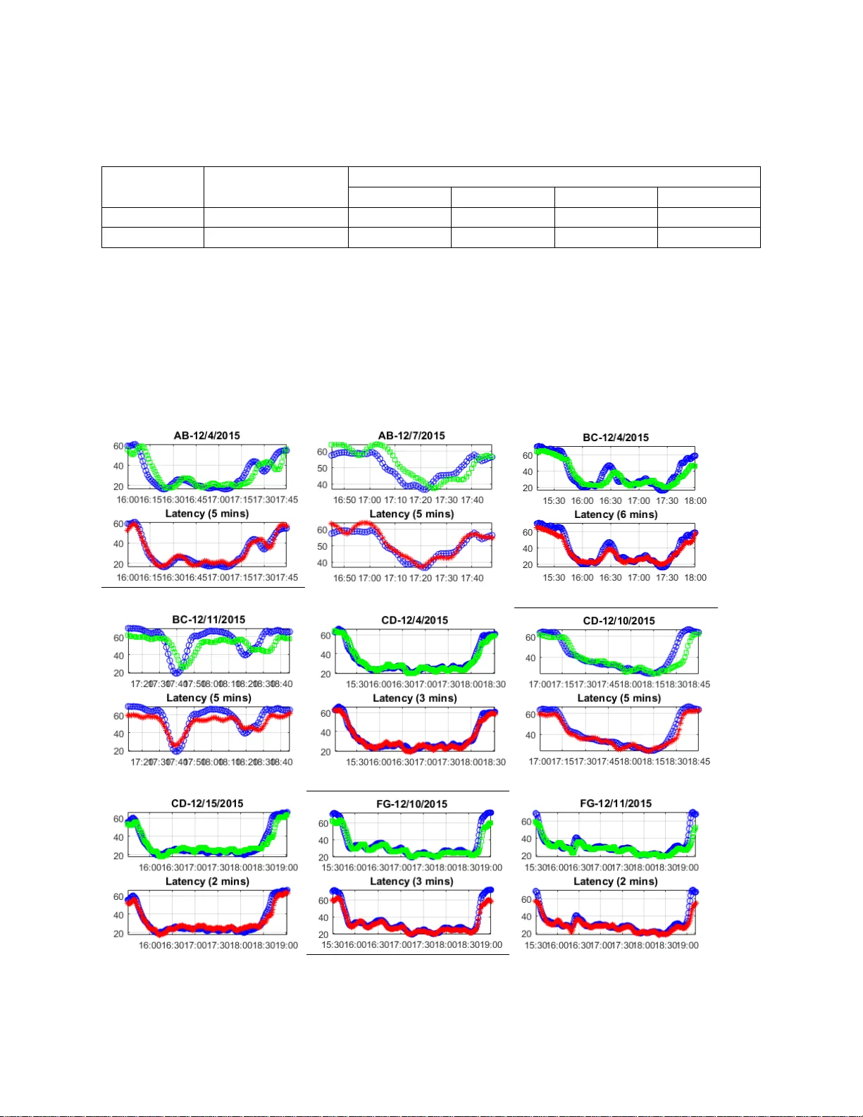
A METHODOLOGY FOR CAL CULA TING THE LA TENC Y OF GPS-PROBE DA T A Zhongxiang W ang Graduate Student Department of Civil & Environmental Eng in eering University of Maryland Email: zxwang25@umd.edu Masoud Hamedi * Senior Research Scientist Center for Advanced T ransportation T echnology University of Maryland 5000 College A ve College Park, MD 20740 Email: masoud@umd.edu | Phone:301-405-2350 Stanley Y oung Advanced T ransportation and Urban Scientist National Renewable Energy Laboratory Email: stanley . young@nrel.gov W ord count: 4,628 words text + (3 tables +8 fig ur es) x 250 words (each) = 7,378 words Submission Date: Aug 1 st , 2016 W ang, Hamedi, Y oung 2 ABSTRACT Crowdsourced GPS probe data has been gaining popularity in rece nt y ears as a source for real - time traf fic information. Effor ts have been made to evaluate the qualit y of such data from dif ferent perspectives. A quality indicator of any traf fic data source is latency that describes the punctuality of data, which is critical for real-time operations, emerg ency response, and traveler information systems. This paper offers a methodology for measuring the probe data latency , with respect to a selected reference source. Although Bluetooth re-identification data is used as the reference source, the methodology can be a pplied to an y other ground -truth data source of choice (i.e. Automatic License Plate Readers, Electronic T oll T ag). The core of the methodology is a maximum pattern matching a l gorithm that works with three dif ferent fitness objectives. T o test the methodology , s ample field reference data were collected on multiple freeways segments for a two-week period using portable Bluetooth sensors as ground-truth. Equivalent GPS probe data was obtained from a private vendor , and its latency was evaluated. Latency at diffe rent times of the day , the impact of road segmentation scheme on latency , and sensitivity of the latency to both speed slowdown, and recovery from slowdown episodes are also discussed. Keywor ds : Latency , GPS -probe data, Bluetooth W ang, Hamedi, Y oung 3 INTRODUCTION Accurate and timel y data is a vital component of a ny Intelligent T ransportation S y stem. In recent years, proliferation of location-aware internet connected devices has enabled private sector to use crowd sou rcing technics for providing network wide r eal-time tr avel time and spee d data for t raf fic management applications. This has re sulted in traffic data services that report speed and trav el time in real-time. This data in turn is used b y private industry for traveler inform ation and routing, and increasingly by public entities as a replacement for field data collec tion a nd to expand observabilit y of roadway conditions network wide. The I-95 Corridor Coalition ’s V ehicle Probe Project has successfully int egrated third party d ata of this nature, commonly referre d to as probe data, for a number of public ag ency applications. Initial concerns about accuracy were addressed by a comprehensive validation prog ram that compared probe industr y reported speeds and tra vel times with those from a se nsor-based reference source. Real-time applica tions are also sensit ive to the latency , that is the time de lay between act ual field conditions, such as a major slowdown, and when it is reflected in the traffic data stream. Appropriate method to benchmark latency is currentl y lacking, and is the focus of this paper . Consumer elec tronics are finding an e ver-increasing role in our everyday lives. A majority of these devices are also equipped with a point - to -point networking protocol commonly referred to as B luetooth. Bluetooth enabled devices can communicate with other Bluetooth ena bled devices anywhere from one meter to about 100 meters. This variabilit y in the communications capability depends on the power rating of the Bluetooth sub-systems in the devices. The Bluetooth protocol uses an electronic identifier , or tag, in each device called a Ma chine Access Control address, or MA C address for short. The MAC address serves as an electronic nickna me so that electronic devices can k eep track of who’s who during data communications. In principle, the Bluetooth traf fic monitoring system calculates travel times by matching public Blueto oth MAC addresses at successive detection stations. B luetooth data has been a ccepted b y the industry as an acc urate and economic solution for collecting ground-truth travel time data. More details on using Bluetooth sensors for freeway travel time data collection is discussed in (1 ). Quality and accuracy of the GPS probe data has been validated mostl y compared to the Bluetooth data by man y researchers. A ve rage A bsolute Speed Er ror and Speed Error Bias are among the quality measures. However , not much effort has be en made to quantify latenc y of the probe data as an indicator of its punctuality . In the context of travel time data, latency can be defined as the dif ference between the time the traf fic flow is perturbed and the time that the change in speed is re flected in the data. When using Bluetooth da ta as ground-truth, latenc y is measured b y observing the time dif ference between the onset of a sl owdown as reported by Bluetooth traffic monitoring, and the time that it is reported by th e GPS probe data. A graphic al representation is shown in FIGURE 1. The time shift between probe data and Bluetooth data, which is marked with orange arr ow , is the latency of GPS probe data. Latency associated with the GPS probe data originates from several sources, and is unavoidable to some extent. Figure 2 shows a co nceptual framework for generating GPS probe data. Ever y second, millions of GPS tracks are being collected and there is a delay from the time that a n observation is made on the field, to the time that it is transmitted through a communication medium to the data collection server . The GPS data is blended with other data sources su ch as historical, incident and weather data and goes t hrough data fusion and filtering en gines, which takes some time. The fused data is then packaged in predetermined form ats and i s inject ed into live feeds fo r consumer c onsumption. The applications running on the user side pull the data. So W ang, Hamedi, Y oung 4 by the time that data is available to the real -time ap plications, traffic d y namics might have changed on the field. It is important to have a good understanding of th e delay , in order to tune the real - time applications. The term ‘latency ’ is used in industry literature in many contexts related to various steps along the proce ssing chain as shown in FIGURE 2. For the purpose of this research, latency is define d a s “ the dif ference between the time the traf fic flow is perturbed a nd the ti me that the change in speed is reflected in the data ”. This represents a system latency – not any specifi c step in the chain. This is the latency that the proposed methodology addresses. FIGURE 1 Measur ement of latency FIGURE 2 GPS-pr obe data processing flow chart W ang, Hamedi, Y oung 5 The paper is organized as following: First a brief review about research on probe data latency is present. Then a methodology , including data processing steps and an iterative matching procedure with three fitness objectives for calculating latency is pres ented. A case study based on extensive field collected Bluetooth and GPS probe data is conducted to test the proposed methodology . In depth anal y sis of the case study results including sensitivity of latenc y to spatial and temporal parameters are presented. Finally , main takeaways and dir ection for future research are summarized. LITERA TURE REVIEW Latency measurement for real-time trave l time data is a relatively untouched research topi c. Haghani et a l. (2) estimated that lag time for GPS-probe data is less than or equal to e ight minutes, however the y did not specify the sourc e for that statement. Liu et al. (3) observed a clear latenc y for reporting GPS-based data as well. Chase et al. (4) further stated that GPS-probe data has greater latency when travel speed recovers after peak p eriod, than the beginning of a p eak period. None of these papers proposed a detailed quantitative la t ency mea surement methodology . Kim a nd Coifman (5) measured the latency for GPS-probe data c ompared to loop detector . They calculated the correlation coefficient, whic h significantly dep ends on the covariance of original time-series speed data and shifted time-series speed data. The results show that the average latency for GPS -probe data is 6.8 minutes, and it could exceed 10 minutes in many sit uations. However , loop detector can onl y report spot travel speed whereas GPS probe data is reported on standardized segments, ty pic ally T raffic Message Control (TMC) industry standard segments. The speed reported is more related to the space mean speed across a TMC segment rather than a spot speed from loop d etectors. Moreover , Kim and Coifman shifted the GPS-probe data in 10 s econd increments. However , the granularity of commerciall y available GPS probe data is one minute or more. METHODOLOGY The methodology used in this paper for quantifying latenc y o f the probe data with respect to Bluetooth data involves multiple steps. The following sections provide a brief description for each step. It would be good t o have a succinct overvi ew of the steps here suc h as – data preparation, filtering, data interpolation and smoothing. The method used compares a reference data source (Bluetooth re-identification data) that directly sa mples travel time on a segment basis, converts the travel times to speed measures, and then compares the speed to that reported b y probe d ata sources. An error metric is calculated between the Bluetooth reference data and the industry prob e data. The probe data is then time shifted until minimum error is achieved. The time-shift that c reates the minimum error is the latency of the data. V arious steps address data preparation (outliers, smoothing, etc.) but the basic approach is as de s cribed. Bluetooth Data Pr eparation Bluetooth sensors store t he MAC ID of the detected Bluetooth devices along with their detection time in a removable memory card. The collected data are downloaded to a server for processing at the end of deployment. The MAC addresses for a ll devices that a re detected between two consecutive sensors are matched to d evelop a sa mple of travel time for that particular segment of the roadwa y . The reader is reminded that travel time and speed are inverse l y related and throughout this paper , they have been used interchangeably . It should be noted that the conversion to spee d is based on the measured distance between sensor locations. I n order to establish the ground truth for W ang, Hamedi, Y oung 6 travel time, individual observations must be aggregated in specified ti me intervals which in this paper are assumed to be equal to one mi nute. I t must also be noted that the detection time of the second sensor is used a s the time label for the individual observations. Space mean speed for each interval is equal to summ ation of travel time of all observations divided b y product of number of observations b y the se gment length. It should be noted that the time reference used in this data is the time when vehicles are re-identified at the downstream sensor (as op posed to the upstream sensor , or the mean time of the upstream and downstream.) This will be discussed in more detail later . Data Filtering Due to the nature of traf fic movement, some data points obtained in the matching stage a re, in fac t, unacceptable due to several reasons. For example, i f after dete ction b y the first sensor , a driver pulls over to replace a flat tire, after reaching the second sensor a travel time observation will be generated that is not a valid representation o f average traffic pattern. In summary , d ata samples with the following characteristics must be identified:  Observations with unreasonably low speeds,  Observations in a particular time interval that are far from the average of the rest of the speeds observed in the same time interval to avoid erra tic variations, and,  Presence of a small number of observations in a time interval that is not enoug h to establish a reliable “ground truth” speed. T o address each of the m entioned potential problems, a series of filters were sequentially applied to the pool of unfiltered observa tions that result from the matching step. V ariations in speed observations are conside red to identif y outlier speed observations. T o that end, all observations corresponding to each o f the time intervals for which we have Bluetooth observations are identified and the average and st andard deviation of the spe eds in those time interva ls are calcula ted. Observations that corres pond to speeds falling within ±1.5 times the standard devi ation are kept and the rest are discarded. Assuming a normal di stributi on for the observ ations around the mean, this approach translates into keeping nearl y 87 percent of the data. T o ensure that the variability among speed observations inside a g iven time interval is within a reasonable le vel, the coef ficient of variations (COV) of Bluetooth spee d observations in each time interval that survive the previous step is estimated, then time intervals that have a COV greater than 1 are excluded and their corresponding observations are discard ed from further consideration in the ground truth estimation process. More details on Bluetooth data m atching and filtering are reported in (1). Man y of the assumptions and procedures for filtering are bas ed on a speed dist ribution with little short -term volatility . If two distinct speed distributions occur on a roadway (as is sometimes experienced, particularly on si gnalized roadways, much -less so on freeways), the methodology should b e used with caution. Interpolation The third step is to interpolate so that the time-series data would have continuous coverage with one aggregated da ta point per each minute. The average of neighboring observations is considered to be the travel speed for the missing interval: W ang, Hamedi, Y oung 7   1 1 t i t t n t i s s s s n        ( 1) Assuming that th ere are n consecutive mi ssing d ata points starting from time t , equation (1) is used to fill the gap between ti me t and t+n . In order to preserve the consistency and integrity of the original data, it was chosen to use the gap filling for mula only when not more than five consecutive data points are missing. Any sample data with larg er than five-minute data gaps were ex cluded from the analysis. The interpolation procedure was applied to both Bluetooth and GPS probe data sets. Smoothing The final step is smoothening o f the raw data. This procedure minimiz es sudden sharp spikes in the g eneral data tre nd caused by randomness of traf fic speeds. Smoother curves allow comparison of the dominant pattern of the data curves, in order to calculate hori zontal offse t corresponding to the ti me gap. The filter fu nction fi ltfilt in Matlab used to conduct the smoo thing is based on rational transfer function, proposed by Oppe nheim, Ronald and John (6) , which is shown as in Equa tion 2. 1 1 ( 1 ) (2) ... ( 1 ) ( ) ( ) 1 (2) ... ( 1 ) b a n b n a b b z b n z Y z X z a z a n z              (2) where a n is the fee dback filter order and b n is the feedforward filter order . When (2) a to ( 1 ) a an  are all zeros, this function dege nerates into weig hted moving average. ( 1 ) b , …, ( 1 ) b bn  are the wei ghts for eac h data in the moving window . The movi ng average function becomes as the following function. ( ) ( 1 ) ( ) (2) ( 1 ) ... ( ) ( 1 ) y k w x k w x k w n x k n        (3) () yk is the smoothed data at time k , ( 1 ) w is the weight for its corresponding data. The moving time window is set to be five minutes. Each smoothed data point will be the su mmation of its weighted original data and weighted previous five minutes data points. One concern with smoothing is that it will shift the curve ba ckward and therefore int roduce an additional delay comparing to original data and as such the measured latenc y would be artificiall y hig her than what is should be. T o solve this problem, smoothing is applied to the raw dat a twice. First forward smoothing is done b y moving the smoothi ng window forward, and then the smoothing is applied backwards with the same weight parameters which compensates the artificial latency . Latency Measur ement Calculating the latency is an iterative process with a time offset, starting from a lower bound and repeating until reaching the pre set upper bound. The underlying assumption is that probe data has the latenc y as explained in the introduc tion. The methodology to measure the latency is to find the best time shift which results in maximum match of Bluetooth curve and probe data curve. Three dif ferent fitness objec tives are applied: Absolute V ertical Distance ( f1 , A VD ), Square V ertical Distance ( f2 , SVD ), and Correlation ( f3 , COR ) . Absolute V ertical Distance ( f1 ) is the absolute value W ang, Hamedi, Y oung 8 of the subtra ction of Bluetooth travel speed and probe data tr avel sp eed over the desired measuring period. Square V ertical Distance ( f2 ) is the square of that subtraction, which gives more weights to the points that have bigger dif ference. Correlation ( f3 ) is a statistical representation of the linear relationship between two curves (7), which is defined as follows: [( )( )] ( , ) BT probe t t latency BT probe t t latency BT probe t t latenc y S S BT probe t t late ncy S S E S S corr S S         (4) Where BT t S is the Bluetooth travel speed without shifting, pr obe t la ten cy S  is probe data travel speed shifted by the latency , E is the expected values, BT t S  , probe t latency S   are ex pected valu es of BT t S and pr obe t la ten cy S  and BT t S  , probe t latency S   are the standard deviations of two curves. The methodology sta rts from the lower bound (no latency , which means time offset is 0), increas es time of fset by 1 minute for each iteration, a nd then calculates all three fitness objectives . After reaching the upp er bound for the ti me of fset, the of fset that results in best fit over all it erations is considered to be the latency . The formulation to find the shift distance which provides the most overlapping data is :   1 2 1 min 1 = min 2 = min 3 = corr( , ) n BT probe data t t latency t n BT probe data t t latency t BT probe data t t latency f S S f S S f S S lb latency ub           ( 5) T o measure the latency of the probe data, both travel speed and trave l time can be used. In order to make the objective metric to the seg ment leng th, this paper uses the former . If the Bluetooth data and GPS -probe data curves sho w the ex act same pattern, shifting the probe curve will eventually result in a perfect m atch with z ero vertical dist ance and c orrelation equals to 1 . However , it is ver y unlikel y due to random nature of traffic movement and also instrumentation error in both Bluetooth and probe tec hnologies. The spe ed observations show less fluctuation during peak periods and heavy congestion conditions. CASE STUDY In order to test this methodology , two freewa y corridors in South C arolina are sele cted. The first section is a 7.07-miles-long segment on I-85, from Exit 48 ( US -276) to Exit 54 (Pelham Rd), which is shown in FIGURE 3 The second section is a 4.67-miles-long se gment on I-26 from Ex it 103 (Harbison B lvd) to Exit 108 (Bush River Rd ), which is shown in FIGURE 3 The data was collected for both westbound and eastbound for I-26 and both northbound and sout hbound for I-85 from December 3, 2015 to December 15, 2015. These two paths are freeway where traffic would not be interrupted b y traffic signals. Small blue dots show the location of Bluetooth sensors. T raffic Message Channel (TMC) codes used b y probe data vendors to report data are also shown on the W ang, Hamedi, Y oung 9 map. T o improve quality of Bluetooth data, two sensors are deployed at each point, with one sensor on the outermost shoulder of each direction. In total 18 Portable Bluetooth se nsors were deployed. Bluetooth sensors a re ma rked b y r ed capital lette rs, and a directional Bluetooth segment consists of data obtained from beginning and end sensor (i.e segment AB is the road segment starting from A and ending at B). GPS probe data was used in this study was ac quired from a priv ate vendor , in one minute granularity . (a) (b) FIGURE 3 Selected study ar ea Then data is smoothed by the weighted moving average method discuss ed earlier . The moving window is set to be five minutes. Only p revious data points are considered. Equation 6 depicts the weights and parameters used for smoothi ng. An example of smoothing of Bluetooth data is graphically shown in FIGURE 4(a) and similar for smoothing of GPS -probe data at FIGURE 4(b). Th e weights arithmetically decrease with respect to the increase of the time dif ference from the smoothing data point to the previous data point. ( ) 0. 33 ( ) 0. 27 ( 1 ) 0.2 0 ( 2 ) 0.1 3 ( 3 ) 0.0 7 ( 4) y k x k x k x k x k x k          (6) After appl y ing the latency m easurement methodology , the laten cy is calculated and visualized on comparative graphs. FIGURE 4(c) is the original travel speed comparison between Bluetooth data and GSP-probe data and FIGURE 4 (d) depicts the same comparison after compensating latenc y (5 mi ns in this scenario) f or GPS -probe data. It m ust be iterated that this number is onl y for on e slowdown episode, on on e segment of the ro ad. In order to have a good understanding of the latency , it is important to apply the methodolo gy to a lar ge number of ca ses on dif ferent road segments, which is conducted later in the study Latency at Peak Periods T o test the methodolog y on all segments, 32 morning peak period showdown episodes and 45 afternoon peak period showdown episodes are observed and identified. All other obse rvations that happened on weekends and off-peak, or with data gap, or with different pattern between B luetooth data and probe data, or the ones that did not exhibit clear slowdown p attern were excluded. The corresponding v endor T MC segments were selected and assigned to the location of Bluetooth sensors. If the Bluetooth sensor location does not match the ex act TMC endpoint, the TMC is assigned to two adjacent seg ments based on the length of each part. The matching error is controlled to be less than 0.01 miles. W ang, Hamedi, Y oung 10 (a) (b) (c) (d) FIGURE 4 Example of travel speed smoothing and latency measur ement (5 minutes) of segment AB during after noon peak at Dec 4 th 2015 (a: Bluetooth data smoothing; b: probe data smoothing; c: original Bluetooth and pr obe data comparison; d: travel speed comparison of Bluetooth data and latency compensated pr obe data). T ABLE 1 shows the average latency calculated based on all identified slowdown episodes , for both morning peak periods and afternoon periods , and based on all three different fitness objectivizes. It can be s een that the avera ge laten cy measured b y three dif ferent fitness objectives are reall y similar to each other , which demonstrates the ef fectiveness of this methodology and that average latency measurement is “ converged”. Therefore, this paper uses the average of the latency calculated b y thre e objecti ves as the G PS -probe data latency . The average probe data laten cy is 4.26 minutes in the morning peak pe riods and 3.94 minutes in the afternoon peak periods. Morning and afternoon peak cases combined, for th ese segments at identified episodes, probe data has an averag e latenc y of 4 minutes. Although latency at morning peak is slightly higher than that in the W ang, Hamedi, Y oung 11 afternoon, there is no significant dif ference. T ABLE 1 A verage latency and evaluation Period Number of Observations A verage Latency (minut e) f1 (A VD) f2 (SVD) f3 (COR) A verage Morning 32 3.96 4.42 4.41 4.26 Afternoon 45 3.64 4.01 4.19 3.94 Several graphical example of afternoon latency comparison of original pr obe data and shifted probe data are shown in FIGURE 5. In the first row , the blue curve represents the Bluetooth data, with the segment name a nd date shown on top and the original probe data shown a s the green curve. Graphs on the second row , show the Bluetooth data and shifted probe data, with resulting latency offset shown on top. The horizontal axis on both graphs shows the time of day , and the vertical axis is travel speed in MPH. Additional rows in this figure show more examples for other segments of dif ferent days. (a) (b) (c) (d) (e) (f) (g) (h) (i) FIGURE 5 Comparison of original GPS-probe d ata and shifted GP S-p r obe data against Bluetooth data W ang, Hamedi, Y oung 12 FIGURE 6 shows the probe data latency distribution. Ass illustrated, the 4 minutes has the highest latenc y distribution densit y and the laten cy distribution is roug hl y symmetric. The mornin g peak fi gure (F I GURE 6a ) and afternoon figure (FIGURE 6b ) have similar dist ributions, which further proofs the similarity of latency at morn ing p eak periods and afternoon peak periods. FIGURE 6(c) is the cumul ative latenc y distribution, which demonstrates that 95% of latenc y values fall with in 6 minutes for both morning peak periods and afternoon peak periods. (a) (b) (c) FIGURE 6 GPS-pr obe data latency distribution (a: latency distribution at morning peak periods; b: latency distribution at afternoon peak periods; c: cu mulative distribution o f G PS- pr obe data) Latency on Differe nt Segments Latencies are also calculated on dif ferent segments to investigate the impact of seg ment length on latency . T A BLE 2 shows the GPS-probe latencies on dif ferent segments ranging from 1.17 mi les to 2.20 miles. The average latency is 4.31 minutes, which is consistent with the probe data latenc y from the previous an alysis. The latencies for different segments vary in a s mall range. The length W ang, Hamedi, Y oung 13 of TMC se gment does n ot seem to have a significant impact on probe dat a latency in thi s stud y . The scattered plot of latency points in F I GURE 7 also shows that the latency is not significantl y correlated with the length of the segment. However , in rural areas some TMC seg ments might be a lot longer than what it is used in this research which may influence th e latency . T ABLE 2 Pr obe data latency at different se gments Segment Length (mile) Average Latency (minute) f1 (A VD) f2 (SVD) f3 (COR) A verage BC 1.17 4.80 5.00 5.00 4.93 KL 1.28 4.43 4.86 5.00 4.76 LM 1.60 3.33 3.83 3.83 3.66 OP 1.64 4.67 5.00 5.00 4.89 AB 1.69 4.56 4.56 4.67 4.60 PQ 1.70 4.78 4.89 4.89 4.85 MN 1.78 4.00 4.18 3.95 4.04 GH 2.02 3.40 3.40 3.00 3.27 CD 2.07 3.92 4.50 4.50 4.31 FG 2.20 2.76 4.06 4.59 3.80 Average for all segments 1.72 4.06 4.43 4.44 4.31 FIGURE 7 Scatter ed plot of p r obe data latency at differ ent length segments Latency at Slowdown and Recovery Observations from the empirical work suggest that the latenc y of GSP-probe data se ems to be asymmetrical when comparing the speed reduction period of a slowdown episode to the speed recovery period of the same episode. An example is provided in FIGURE 8 for segment CD during W ang, Hamedi, Y oung 14 afternoon peak period. As illustrated, the slowdown episode in broke n into t wo parts. The fir st part starts when the speeds start to decline, and e nds at the transition time whe n speeds start to recover . The transition time is the time that speeds have reached a minimum value during the episode. It must be noted that since the Bluetooth data is used as reference, the minimum speed used to determine the transition time corresponds to the Bluetooth data. The second part of the slowdown episode starts at th e speed transition point, and ends when speed fully r ecovers to the fre e flow level. T o test the as y mmetrical latenc y h ypothesis, a total of 77 speed slowdown episodes were analyzed. For each slow down episode, the start time of the slowdown, the time of the minimum speed, and the end time of the episode when speeds r ecover w ere identified. The same methodology discussed p reviously in the paper w as applied to the slowdo wn and recover y parts of the data separately . T ABLE 3 shows a summary of the results for all 77 cases. I t can b e observed that in g eneral, probe data exhibits smaller latency in ca pturing reduction of s peeds both in morning and afternoon peak. The ave rage latency for ca ptu ring slowdown is 3.68 minutes compared to 4.83 minutes for capturing the speed r ecovery during the morning peak. Similarly in the afternoon peak, probe d ata captures slowdown with 3.54 minute la tency which is lowe r than 4.76 minute of latency for capturing the speed recovery . I n general, the probe da ta has shown 3.60 minutes of latency for capturing the speed slow down compared to 4.79 minutes for capturing the speed recover y when all 77 cases ar e considered as shown in the last row of T ABLE 3. In other words, si gnifica nt reduction in traffic speed seems to be reflected in probe data with 25% less latency compared to the recovery from slowdowns. FIGURE 8 Exa m ple of asymmetry of probe data latency during travel sp eed slowdown and r ecovery periods W ang, Hamedi, Y oung 15 T ABLE 3 Latency at slowdown and r ecovery Tim e Period Scenario Number of Observations A verage Latency (minute) f1 (A VD) f2 (SVD) f3 (COR) A verage Morning Slowdown 32 3.55 3.60 3.90 3.68 Recovery 32 4.76 5.15 4.45 4.83 Afternoon Slowdown 45 3.43 3.45 3.75 3.54 Recovery 45 4.70 4.94 4.62 4.76 Overall Slowdown 77 3.48 3.51 3.81 3.60 Recovery 77 4.72 5.03 4.55 4.79 CONCLUSION This paper make s a n ef fort to analyze and qua ntify latency associated with GPS probe data compared to Bluetooth traf fic data. Several data cleaning and processing methods are described to prepare d ata step b y step. After interpolating da ta and smoothin g the time series, an iterative procedure is discussed to calcula t e the latency by finding the time shif t that maximizes the overlapping of Bluetooth and GPS probe data b ased on three different fitness objectives. T wo freeway corridors were s elected to conduct th e case stud y and test the methodology . Results of case study show that the methodolog y has be en successful for measu ring the latency of th e probe data. It is shown th at the latenc y of probe data in capturing slowdowns is less compared to the latency for capturing speed recovery . The len gth of the segment does not seem to impact the latency value in the studies scenarios. Further res earch is required to investigate the impact of smoo thing meth od on latenc y measurement. The methodology is robust onl y if short term volatilit y in traffic pattern is limited , and thus cannot be applied to measure latency o n arterials with high speed fluctuations due to signal timing and mid -block friction factors. Further research is required to design and appl y pattern matc hin g algorithms to such c ases. The beginning, transition and end time of each slowdown episode in thi s stud y were identified manually using a combi nation of visual graph inspection and statisti cal analysis which is v ery tedious. Authors are working tow ards a methodology for automatic identification of showdowns and their characteristics that is crucial for applying the latenc y assessment approach on future case studies. Obtaini ng data from multiple probe data vendors and analyzing laten cy on different freeways facilities is also subj ect of future research. The r esults pr esented in t his paper ar e based on d ata that is limited in time and scope, and thus they ar e not conclusive and do not r epr esent the state of latency in com mer cial pr ob e data in general . Nonetheless the methodology is prov en to be ef fective and a step in right direction for quantifying the latency of the GPS-probe data. ACKNOWLEDGEMENTS Data used in this study was collected b y the I-95 Corridor Coalition as par t of their V ehicle Probe Pr oject. The r esults and conclusions in this docu ment are those of the author s and not th e I-95 Corridor Coalition. REFERENCES 1. Haghani, A, et al. "Data collection of freeway travel time g round truth with Bluetooth sensors." Transportation Research Record: Journal of the Transportation Research W ang, Hamedi, Y oung 16 Board 2160 (2010): 60-68. 2. Haghani, A., Hamedi, M., Sadabadi, K. I-95 Corridor Coalition Vehicle Probe Project: Validation of Inrix Data July-September 2008, Final Report, I-95 Corridor Coalition. 2009 3. Liu, X, Chien, S., and Kim K. "Evaluation of floating car technologies for travel time estimation." Journal of Modern Transportation 20.1 (2012): 49-56. 4. Chase, R., et al. "Comparative eva luation of reported speeds from co rresponding fixed-point and probe-based detection systems." Transportation Rese arch Record: Journal of the Transportation Research Board 23 08 (2012): 110 -119. 5. Kim, S., and Coifman, B. "Comparing INRIX speed data against concurrent loop detector stations over several months." Transportation Research Part C: Emerging Technologies 49 (2014): 59-72. 6. Oppenheim, Alan V., Ronald W. Schafer, and John R. Buck. Discrete-Time Signal Processing. Upper Saddle River, NJ: Prentice-Hall, 1999. 7. Rodgers, J. L.; Nicewander, W. A. (1988). "Thirteen ways to look at the correlation coefficient". The American Statistician 42 (1): 59 – 66.