Graph Spectral Image Processing

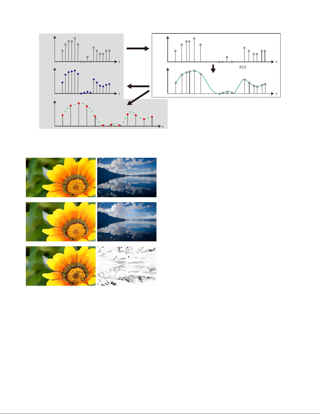
SUBMITTED TO PR OCEEDINGS OF THE IEEE 1 Graph Spectral Image Processing Gene Cheung, Senior Member , IEEE, Enrico Magli, F ellow , IEEE, Y uichi T anaka, Member , IEEE, and Michael Ng, Senior Member , IEEE Abstract —Recent advent of graph signal processing (GSP) has spurred intensive studies of signals that li ve naturally on irregular data kernels described by graphs ( e.g. , social networks, wireless sensor networks). Though a digital image contains pixels that reside on a r egularly sampled 2D grid, if one can design an appropriate underlying graph connecting pixels with weights that reﬂect the image structure, then one can interpr et the image (or image patch) as a signal on a graph, and apply GSP tools for processing and analysis of the signal in graph spectral domain. In this article, we overview recent graph spectral techniques in GSP speciﬁcally for image / video processing. The topics cov ered include image compr ession, image restoration, image ﬁltering and image segmentation. Index T erms —Image processing, graph signal processing I . I N T RO D U C T I O N Graph signal pr ocessing (GSP) is the studies of signals that liv e on irregularly structured data k ernels described by graphs [1], such as social networks and wireless sensor networks. The underlying graph typically re veals signal structures; an edge ( i, j ) with large weight w i,j connecting nodes i and j means that the signal samples at i and j are expected to be similar or correlated. Though a digital image contains pixels that reside on a regularly sampled 2D grid, one can nonetheless interpret an image (or an image patch) as a signal on a graph, with edges that connect each pixel to its neighborhood of pixels. By choosing an appropriate graph that reﬂects the intrinsic image structure, a spectrum of graph frequencies can be deﬁned through eigen-decomposition of the graph Laplacian matrix [2], and notions like transforms [3]–[8], wavelets [9]–[11], smoothness [12]–[16] etc can be correspondingly derived. Then a target image (or image patch) can be decomposed and analyzed spectrally on the chosen graph using de veloped GSP tools—analogous to frequency decomposition of square pixel blocks via known transforms like discrete cosine transform (DCT). Recently , this graph spectral interpretation of traditional 2D images has led to ne w insights and understanding, resulting in optimization of both the underlying graph and the graph-based processing tools that shows demonstrable gain in a number of traditional image processing areas, including image compression, restoration, ﬁltering and segmentation 1 . For image compression, a F ourier-like transform for graph- signals called graph F ourier transform (GFT) [1] and many Manuscript receiv ed August 30, 2017; re vised November 30, 2017. Y . T anaka was supported in part by JSPS KAKENHI under Grant Number JP16H04362 and JST PRESTO under Grant Number JPMJPR1656. M. Ng was supported in part by HKRGC GRF 12302715, 12306616 and 12200317, and HKBU RC-ICRS/16-17/03. 1 W e note that while graph has been used extensi vely as an abstraction for image processing in the past [17], we focus in this article in particular recent dev eloped techniques that process or analyze image signals in appropriately chosen graph spectral domains. variants [5]–[8], [18], [19] have been used as adaptiv e trans- forms for coding of piecewise smooth (PWS) and natural images. Because the underlying graph used to deﬁne GFT can be different for each code block, the cost of describing the graph as well as the cost of coding GFT coefﬁcients to represent the signal must both be taken into consideration. For wa velets on graphs [9]–[11], where the conv entional notion of “do wnsampling by 2” is ill-deﬁned for irregular data kernels, ho w to deﬁne critically sampled perfect reconstruction ﬁlterbanks (with (bi)orthogonal conditions) using appropriate downsamplers has been a challenge. W e re view proposals in designs of graph transforms and wav elets for image / video compression in Section III. For image restoration such as denoising and deblurring, how to design appropriate signal priors to regularize otherwise ill-posed problems is a major challenge. Notions of sparsity [20] and signal smoothness [13], [16], [21], [22] can also be generalized to the graph-signal domain. W iener ﬁltering for graph-signals, which ﬁrst requires a proper deﬁnition of wide sense stationarity for irregular graph data kernels, was recently dev eloped [23]. W e revie w popular graph-based restoration techniques in Section IV. Spectral ﬁltering is a fundamental image processing op- eration. It turns out that the well-kno wn bilateral ﬁlter for image denoising [24] can be interpreted as a linear low- pass ﬁlter for a speciﬁc graph [25]. Other diffusion and edge-preserving smoothing operators are also discussed in Section V. Popular applications such as image retar geting and non-photorealistic rendering of images are also overvie wed. Finally , fast implementation of graph ﬁlters using Chebyshev polynomial approximation is discussed. Image segmentation is an old computer vision problem, and there is a long history of graph-based approaches such as graph cuts [26], [27]. More recent models such as the Mumford- Shah model [28] and graph biLaplacian [29] are discussed in Section VI. I I . P R E L I M I NA R I E S A. Graph Deﬁnition W e ﬁrst introduce common deﬁnitions and concepts in GSP for use in later sections. A graph G ( V , E , W ) contains a set V of N nodes and a set E of M edges. Each existing edge ( i, j ) ∈ E is undirected and contains an edge weight w i,j , which is typically positive; a large positive w i,j would mean that samples at nodes i and j are expected to be similar / correlated. Common for images, weight w i,j of an edge connecting nodes (pixels) i and j is computed using a Gaussian kernel, as done in the bilateral ﬁlter [24]: w i,j = exp  − k l i − l j k 2 2 σ 2 l  exp  − k x i − x j k 2 2 σ 2 x  (1) SUBMITTED TO PR OCEEDINGS OF THE IEEE 2 where l i is the location of pixel i on the 2D image grid, x i is the intensity of pixel i , and σ 2 l and σ 2 x are two parameters. Hence 0 ≤ w i,j ≤ 1 . Larger geometric and/or photometric distances between pixels i and j would mean a smaller weight w i,j . Edge weights can alternatively be deﬁned based on local pixel patches, features, etc [30]. T o a large extent, the appropriate deﬁnition of edge weight (inter -node similarity) is application-dependent; we will introduce various deﬁnitions for different applications in the sequel. More generally , a suitable graph can be constructed from a machine learning perspective—gi ven multiple signal observa- tions, identify a graph structure that best ﬁts the observed data giv en a ﬁtting criterion or model assumptions [31]–[34]. For example, graphical lasso in [31] computes a sparse in verse cov ariance matrix (precision matrix) assuming a Gaussian Markov Random Field (GMRF) model and a sparse graph. Graph learning is a fundamental problem in GSP and is discussed extensiv ely in another article in this special issue. A graph-signal x on G is a discrete signal of dimension N —one sample x i ∈ R for each node 2 i in V . Assuming nodes are appropriately labeled from 1 to N , we can treat a graph-signal simply as a vector x ∈ R N . B. Graph Spectrum Giv en an edge weight matrix W where W i,j = w i,j , we deﬁne a diagonal de gr ee matrix D , where d i,i = P j W i,j . A combinatorial graph Laplacian matrix L is L = D − W [1]. Because L is symmetric, one can sho w via the Spectral Theorem that it can be eigen-decomposed into: L = UΛU T (2) where Λ is a diagonal matrix containing real eigenv alues λ k along the diagonal, and U is an eigen-matrix composed of orthogonal eigen vectors u i as columns. If all edge weights w i,j are restricted to be positive, then graph Laplacian L can be proved to be positive semi-deﬁnite (PSD) [2] 3 , meaning that λ k ≥ 0 , ∀ k and x T Lx ≥ 0 , ∀ x . Non-negati ve eigen values λ k can be interpreted as graph fr equencies , and eigenv ectors U interpreted as corresponding graph frequency components. T ogether they deﬁne the graph spectrum for graph G . The set of eigenv ectors U for L collecti vely form the graph F ourier T ransform (GFT) [1], which can be used to decompose a graph-signal x into its frequency components via α = U T x , similar to known discrete transforms such as DCT . In fact, one can interpret GFT as a generalization of known transforms like DCT ; see Shuman et al. [1] for details. Note that if the multiplicity m k of an eigen value λ k is larger than 1, then the set of eigen vectors that span the corresponding eigen-subspace of dimension m k is non-unique. In this case it is necessary to specify the graph spectrum as the collection of 2 If a graph node represents a pixel in an image, each pixel would typically have three color components. For simplicity , one can treat each color component separately as a different graph-signal. 3 One can prove that a graph G with positive edge weights has PSD graph Laplacian L via the Gershgorin circle theorem: each Gershgorin disc corresponding to a row in L is located in the non-negati ve half-space, and since all eigenv alues reside inside the union of all discs, they are non-negati ve. eigen vectors U themselves. See more discussion on this issue in the compression context in Section III. If we consider also negativ e edge weights w i,j that reﬂect inter-pix el dissimilarity / anti-correlation, then graph Laplacian Ł can be indeﬁnite. W e discuss a few recent w orks that employ negati ve edges in Section IV. C. V ariation Operators Closely related to the combinatorial graph Laplacian Ł are other variants of Laplacian operators, each with its own unique spectral properties. A normalized graph Laplacian Ł n = D − 1 / 2 Ł D − 1 / 2 is a symmetric normalized variant of Ł. In contrast, a random walk graph Laplacian Ł r = D − 1 Ł is an asymmetric normalized variant of Ł. A generalized graph Laplacian Ł g = Ł + diag( d i,i ) is a graph Laplacian with self-loops d i,i at nodes i —called loopy graph Laplacian in [35]—resulting in a general symmetric matrix with non- positiv e off-diagonal entries [36]. Eigen-decomposition can also be performed on these operators to acquire a set of graph frequencies and frequenc y components. For e xample, normalized v ariants Ł n and Ł r share the same eigen v alues between 0 and 2 . While Ł and Ł n are both symmetric, Ł n does not have the constant vector as an eigen vector . Asymmetric Ł r can be symmetrized via left and right diagonal matrix multiplications [37]. W e will discuss dif ferent choices of variation operators in the sequel for different applications 4 . D. Graph-Signal Priors T raditionally , for graph G with positive edge weights, signal x is considered smooth if each sample x i on node i is similar to samples x j on neighboring nodes j with large w i,j . In the graph frequency domain, it means that x contains mostly low graph frequency components; i.e. , coefﬁcients α = U T x are zeros for high frequencies. The smoothest signal is the constant vector —the ﬁrst eigenv ector u 1 for L corresponding to the smallest eigen value λ 1 = 0 . Mathematically , we can write that a signal x is smooth if its graph Laplacian r e gularizer x T Lx is small [14]–[16]. Graph Laplacian regularizer can be expressed as: x T Lx = X ( i,j ) ∈E w i,j ( x i − x j ) 2 = X k λ k α 2 k (3) Because L is PSD, x T Lx is lower -bounded by 0 , achiev ed when x = c u 1 for some scalar constant c . In [12] the adjacency matrix W is interpreted as a shift operator , and thus graph-signal smoothness is deﬁned instead as the dif ference between a smooth signal x and its shifted 4 In [38], a general denoising regularization term is proposed where the penalty is proportional to the inner product between the signal x and its denoised residual x − f ( x ) ; x T Ł x being an example if I − Ł is interpreted as a denoising operator. The main goal of [38] is to show this regularization term can be used as an engine for more general in verse problems, similar to plug-and-play priors ( P 3 ) [39]. In contrast, our goal here is to sho w different graph variation operators have different characteristics that are suitable for different applications. SUBMITTED TO PR OCEEDINGS OF THE IEEE 3 version Wx . Speciﬁcally , graph total variation based on l p - norm is: TV W ( x ) =     x − 1 | λ max | Wx     p p (4) where p is a chosen integer . More speciﬁcally , a quadratic smoothness prior is deﬁned in [13] (also in [38]): S 2 ( x ) = 1 2 k x − Wx k 2 2 (5) Besides smoothness, sparsity of graph-signals with respect to a trained graph dictionary can also be used as a prior [40]. Speciﬁcally , to effecti vely represent signals on different graph topologies, graph atoms are constructed as polynomials of the graph Laplacian. Preliminary results in [40] sho w its potential, but we will not discuss this further in the sequel. I I I . G R A P H - BA S E D I M AG E C O M P R E S S I O N Image compression refers to the process of encoding an image x onto a codeword c ( x ) , minimizing distortion in the reconstructed image b x for a giv en target bit-rate R T , i.e. min D ( x , b x ) sub ject to R ( c ( x )) ≤ R T , (6) where R ( c ( x )) is the av erage codeword length. Traditionally , lossy compression employs a 2D transform (denoted as U ) to produce a ne w image representation where image pixels are at least approximately uncorrelated. This process typically generates a vector of transform coefﬁcients as α = U − 1 x , such that only few coefﬁcients of α are signiﬁcantly differ - ent from zero. This is critical to achiev e good compression performance, and such coefﬁcients can often be interpreted in terms of a frequency representation. A. Adaptive transforms for compr ession More in detail, as in Fig. 1, the ﬁrst step consists of the linear transform generating coefﬁcients α . Such coefﬁcients are subsequently quantized, and the quantization index es are losslessly coded using some data compression algorithm such as Huffman or arithmetic coding. There exist plenty of vari- ations on this scheme, and the interested reader is referred to textbooks on the subject for details, e.g. [41]. For our discussion, it is important to note that, if the transform to be used is not known in advance at the encoder and decoder but it is computed adaptively at the encoder in order to optimize the compression process, then some ancillary information has to be communicated to the decoder, in order to reconstruct the corresponding in verse transform to correctly decode the image. The rate term in (6) can be written as R ( c ( x )) = R α + R O , i.e. the rate needed to encode the transform coefﬁcients plus the ov erhead rate due to the ancillary information; both terms may depend on x , making the design of adaptiv e transforms a challenging problem. In this section we focus on the transform stage, as spectral graph theory pro vides innovati ve tools to design transforms for image compression. Seeking an “optimal” transform has prov ed to be an elusive goal except for a few rather simple image models. The Karhunen-Lo ` eve transform (KL T) is based Tr a n sf o r m ! "# Quantiza tion. +. codin g $ x Tr a n sf o r m adaptation B I T S T R E A M %&'()* $ a ncillary.information %&'()* + ,-./ Fig. 1. Block diagram of lossy compression scheme. Coefﬁcients are transformed, quantized and entropy coded. The transform is signal-adaptiv e, and the bitstream is composed of the coded transform coefﬁcients (rate R α ) plus the ancillary information (rate R O ), for a total rate R ( c ( x )) ≤ R T . on the eigendecomposition of the cov ariance matrix of the input process and is very similar to the principal component analysis; it has been shown to be optimal for a Gaussian source under mean square error metric and ﬁxed-rate coding [42]. The DCT [43] is asymptotically equiv alent to the KL T for a ﬁrst- order autoregressi ve process [44]. Howe ver , these models fail to capture the complex and nonstationary behavior typically occurring in digital images, and transform design is still an activ e research area. While many commonly used transforms, such as the DCT and w avelets [45], emplo y a ﬁxed set of basis vectors that need not be communicated to the decoder , the KL T is a signal-adaptiv e transform. Adaptivity allo ws to match the basis vectors (the columns of U ) to a class of signals of interest, but the transform matrix has to be known at both the encoder and decoder; moreo ver , the resulting transform has no structure and hence lacks any fast algorithm. These issues have limited the practical use of the KL T for signal compression. Like the KL T , the GFT is also based on an eigenv ector de- composition. The GFT interprets a signal as being deﬁned on a graph, and calculates the eigenv ector decomposition of the corresponding graph Laplacian as in (2). Thus, while the KL T takes a statistical approach, describing correlations among image pixels through estimates of their linear correlation coef- ﬁcients, the GFT employs a more ﬂexible approach, in which pixel similarities are encoded into the weights of an undirected graph, where each node of the graph represents a pixel, and each edge weight represents the “similarity” of the two pixels at the ends of the edge. The two transforms are related to each other; in particular , [46] shows that the GFT approximates the KL T for a piece-wise ﬁrst-order autoregressi ve process, while [5] sho ws that the GFT is optimal for decorrelation of an image following a Gauss-Marko v random ﬁeld (GMRF) model. Both the KL T and GFT can be interpreted in terms of kernels. In the KL T , the cov ariance matrix (which is PSD) is obtained from a (PSD) linear kernel, whereas the GFT is obtained from the graph Laplacian matrix, which is also PSD. In practice, ho wev er , a graph can be computed for each individual image, making the GFT a more ﬂexible frame work for transform design. Roughly speaking, the graph in the GFT encodes image structures, as opposed to statistical correlations. This is useful because one can decide the degree of accuracy with which structures are represented in the graph, providing means to reduce the overhead of signaling the transform to SUBMITTED TO PR OCEEDINGS OF THE IEEE 4 (a) (b) (c) Fig. 2. (a) Square grid graph; (b) a 32x32 image block, and (c) an example of graph superimposed onto it. Graph edges with white color denote weak pixel similarity , and the ﬁgure shows that graph edges indeed encode structural information about the image. the decoder . Referring to Fig. 1, using the GFT in a transform coding scheme requires communication to the decoder a description of the graph as ancillary information; the relati vely high ov erhead requires ﬁnding descriptions of the graph that are optimized in a rate-distortion (RD) sense, i.e. they are sufﬁciently informativ e to yield effecti ve transforms, without requiring a large overhead. B. Graph F ourier T ransform and graph design As has been seen in Sec. II-B, the graph topology and set of weights G ( V , E , W ) fully deﬁne the graph Laplacian matrix, from which the GFT is computed 5 . Hence, obtaining a “good” GFT amounts to selecting the topology and weights yielding the best compression performance in an RD sense as in (6). Regarding the topology , giv en that 2D images are typically deﬁned on a square grid, a square grid graph is typically employed as in Fig. 2-a, where each pixel is connected to its four horizontal and vertical neighbors. In principle, one may decide to add graph edges corresponding to diagonal neighbors, or connecting pixels whose distance is larger than one. Howe ver , this may greatly increase the overhead of communicating the graph, unless edges are carefully selected e.g. as proposed in [48]. Fig. 2-b shows a 32x32 image block with the corresponding graph superimposed onto it, emphasizing the fact that the graph encodes image structures. 1) Choosing edge weights: The weight w i,j on each edge of the graph is conv entionally computed as a function of the difference in pix el v alues x i and x j connected by that edge— i.e. the photometric distance—as computed in (1). Howe ver , it is easy to realize that real-v alued graph weights are too expensi ve in terms of overhead. In [3], [49], [50] the weights are constrained to be in the set { 1 , 0 } , implying that the graph only describes strong or zero correlation; the weights are chosen from detected image edges [18], using a greedy optimization algorithm [49], or from the output of an image segmentation algorithm, where an independent graph with weights equal to one is associated to each re gion and the resulting GFT plays the role of a shape-adaptive transform [50]. In [51] the difference | x i − x j | is quantized to two values using a pdf-optimized uniform quantizer, yielding a graph that is always connected by construction; although weight binarization leads to suboptimal compression ef ﬁciency , it is 5 Other approaches are also possible, e.g. [47] deﬁnes a GFT obtained from the eigendecomposition of the graph adjacency matrix. shown that a suitably designed quantizer makes the perfor- mance loss very small. In [46] two sets of weight v alues are used, i.e. w i,j ∈ { 1 , 0 } for image blocks characterized by strong or zero correlation, and w i,j ∈ { 1 , c } for blocks with strong or weak correlation. The constant c is optimized using a model suitable for piecewise smooth signals, and very good results are obtained in the compression of depth map images. The ov erhead incurred by the graph, howe ver , makes it harder to obtain signiﬁcant gains on natural images. This problem is addressed in [51], where edge prediction followed by coding is used to reduce the overhead, leading to performance gains between 1 and 3 dB in peak signal-to- noise ratio (PSNR) over the DCT . More sophisticated graph coding techniques may also be de vised, e.g. one might in principle apply contour coding techniques as in [52], [53] to reduce the cost of representing the graph. Moreover , in [53] directional graph weight prediction modes are proposed, which av oid transmitting any overhead information to the decoder . 2) Graph learning: Deﬁning a good graph from data observations is so important in man y applications, and par- ticularly in compression, that more structured methods have been developed to this purpose; this problem is referred to as graph learning . In [54], the authors formulate the graph learning problem as a precision matrix estimation with gen- eralized Laplacian constraints. In [55], a sparse combinatorial Laplacian matrix is estimated from the data samples under a smoothness prior . In [56], a new class of transforms called graph template transform is proposed; the authors use a graph template to impose a sparsity pattern and approximate the empirical inv erse covariance based on that template. While the methods abov e are effecti ve at deriving a graph from data, none of them takes into account the actual cost of representing, and thus coding, the graph, which is clearly a major problem for image compression. In [57] a nov el graph- based framew ork is proposed, explicitly accounting for the cost of transmitting the graph. The authors treat the edge weights w i,j as a graph signal that lies on the dual graph. They compute the GFT of the weights graph and code its quantized transform coefﬁcients. The choice of the graph is posed as a RD optimization problem. 3) Reducing GFT complexity: Besides the cost required to represent and encode the graph, the complexity of solving (2) to obtain the GFT matrix may outweigh any obtained coding gain. Indeed, applying the GFT to large blocks may quickly become infeasible. In [46] the authors propose to use a lookup table storing the GFTs for the most commonly used graphs, so that only the index of the corresponding chosen transform has to be transmitted; this has been shown to work well for relati vely small block sizes. Moreover , in [4], [46] it is proposed to apply the GFT to a low-resolution version of the image, and to employ edge-adaptive ﬁltering to restore the original resolution. In [58] graph-based separable transforms are proposed, where the transform is optimized sep- arately along ro ws and columns. In [59] symmetric line-graph transforms are proposed, in which symmetries are exploited to reduce the number of operations needed to compute the transform. SUBMITTED TO PR OCEEDINGS OF THE IEEE 5 0.06 0.08 0.1 0.12 0.14 0.16 0.18 25 30 35 40 45 50 Bit per pixel (bpp) PSNR(dB) Teddy MR − GFT MR − UGFT SAW HR − UGFT HR − DCT Fig. 3. Compression performance on the T eddy depth image, employing the MR-GFT [46], the MR-UGFT [4], H.264/A VC in intra mode (HR-DCT), the HR-UGFT [3], and the shape-adaptive wavelet (SA W , [60]). The top line shows reconstruction using the MR-GFT (left) and HR-DCT (right) at 0.1 bpp. 4) Compr ession performance: Sev eral authors hav e applied the GFT for image and video compression. In a practical setting, GFT coefﬁcients over different image blocks may cor- respond to different frequencies (eigenv alues), making entropy coding somewhat more difﬁcult. A possible solution employs bit-plane coding of coefﬁcient signiﬁcance, which depends only on the energy distribution of the transform coefﬁcients. In Fig. 3 we report a comparison on compression of depth images. As can be seen, the MR-GFT codec [46] outperforms the other transforms in rate-distortion sense; in particular , gains between 5 and 10 dB are obtained with respect to the corresponding DCT -based coder . Correspondingly , at the same bit-rate the MR-GFT yields a depth image with less e vident artifacts. C. Steerable transforms fr om GFT In many cases much of the content of an image block can be described by few main structures, employing a simpliﬁed image model with much fewer parameters, leading to reduced ov erhead. In particular, the directional model has become rather popular , e.g. in directional intra prediction modes [61] and directional transforms [62]–[68], including more sophis- ticated transforms such as bandelets [69] and anisotropic transforms [70]. The GFT framew ork can also be employed to design simpliﬁed adaptive transforms. As has been seen in Sec. II, the DCT is the GFT of the line graph with all weights equal to 1. In the same way , the basis vectors of the 2D-DCT are eigenv ectors of the Laplacian of a square grid graph as in Fig. 2 [5], but the solution to (2) for a square grid graph is not unique because the eigenv alues of L do not all ha ve algebraic multiplicity equal to one [71]. Using the pair ( k , l ) with k , l ∈ [1 , n ] instead of index i in (a) (b) Fig. 4. (a) 2D-DCT basis vectors represented in matrix form (with n = 8 ): the corresponding two eigenvectors of an eigenv alue with multiplicity 2 are highlighted in red, the n − 1 eigen vectors corresponding to λ = 4 are highlighted in blue and the n − 1 eigen vectors corresponding to the eigen values with algebraic multiplicity 1 are highlighted in green. (b) Basis vectors of steered 2D-DCT with θ k,l = π 4 ∀ k, l . order to emphasize the bidimensionality of the basis vectors corresponding to the eigenv ectors of L in the 2D case, it is easy to show that λ k,l = λ l,k for k 6 = l , i.e. these eigenv alues hav e multiplicity 2. Moreover , λ k,n − k = 4 for 1 ≤ k ≤ n − 1 , i.e. this eigenv alue has multiplicity n − 1 . Graphically this is shown in Fig. 4(a), where the basis vectors highlighted in red represent an example of eigen vectors corresponding to the same eigenv alue. Therefore, the set of all possible eigenbases satisfying (2) for the Laplacian of a square grid graph can be represented as " u 0 ( k,l ) u 0 ( l,k ) # =  cos θ k,l sin θ k,l − sin θ k,l cos θ k,l   u ( k,l ) u ( l,k )  , (7) where u ( k,l ) are the eigen vectors corresponding to the basis vectors of the separable 2D-DCT . Indeed, (7) applies a rota- tion of an arbitrary angle θ k,l to each pair of basis vectors u ( k,l ) and u ( l,k ) . The new transform is deﬁned by the new eigen vectors u 0 ( k,l ) , or equiv alently and more handily by the original eigen vectors u ( k,l ) plus the set of rotation angles θ k,l . Fig. 4(b) sho ws the resulting set of 2D basis vectors when θ k,l = π 4 ∀ k , l . Such angles must be chosen to match the directional char- acteristics of the image block the transform is applied to, and to minimize the overhead of transmitting the angles. In [71] the same angle is chosen for all pairs of basis vectors with multiplicity equal to 2, i.e. θ k,l = θ . In [57] θ k,l is chosen individually for each pair , almost halving the number of DCT coefﬁcients to be transmitted. In [72] the angles are chosen in a RD optimized fashion. In terms of implementation, in [72] it is noted that the coefﬁcients of the steered transform can be obtained from the coefﬁcients of the separable 2D-DCT of the image block, followed by the application of a sparse rotation matrix; this makes the complexity only marginally higher than that of the separable 2D-DCT . Interestingly , the same principle can be applied to other transforms as well. In [8] it is shown that steerable 1D and 2D Discrete Fourier transforms (DFT) can be obtained. In the one-dimensional case, rotations change the balance of signal energy between the real and imaginary parts of the DFT ; the resulting transform is related to the DCT , the discrete sine transform and the Hilbert transform. In 2D, rotations indeed correspond to geometric rotations. SUBMITTED TO PR OCEEDINGS OF THE IEEE 6 D. Applications W e hav e previously mentioned applications of GFT to the compression of depth maps and natural images. Other authors hav e applied various types of GFT to video compression. In [73] the GFT is optimized for intra-prediction residues, while in [74] the authors propose a block-based lifting transform on graphs for intra-predicted video coding. A graph-based method for inter-predicted video coding has been introduced in [75], where the authors design a set of simpliﬁed graph templates capturing basic statistical characteristics of inter- predicted residual blocks. In [59] symmetric line-graph trans- forms are proposed for predictiv e video coding. In [76] a new edge coding methods is introduced with application to intra prediction residuals. Applications of GFT to other types of data hav e also been presented. In [77] a graph-based representation is applied to the problem of interactive multi view streaming, while in [78] a weighted GFT is employed for compression of light ﬁelds. In [79] the time-varying geometry of 3D point cloud sequences is represented as a set of graphs on which motion estimation is performed, whereas in [80] the graph representation is used to encode luminance information in multivie w video. Finally , a few works hav e employed graph wa velets to im- age/video coding problems. In [81] a graph wav elet transform has been proposed for image compression. In [82]–[84] the authors propose a complete video encoder based on lifting- based wav elet transforms on graphs; constructing a graph in which any pix el could be linked to sev eral spatial and temporal neighbors, they jointly e xploit spatial and temporal correlation. In [85] lifting-based graph wav elets are applied to compression of depth maps. In [86] graph wa velets are employed for the compression of h yperspectral images. These 3D images are characterized by a signiﬁcant amount of correlation among images at dif ferent wa velengths, as well as spatial correlation, which are exploited constructing a spatial-spectral graph for groups of bands. I V . G R A P H - BA S E D I M AG E R E S T O R A T I O N Image restoration is an inv erse problem; giv en a noise- corrupted and/or degraded observation y , one is tasked with restoring the original signal x . Examples of restoration prob- lems include image denoising, interpolation, super-resolution, deblurring, etc. An example generic image formation model is: y = Hx + z (8) where H is a de gradation matrix that performs down-sampling, blurring etc., and z is an additiv e noise. Image restoration is an ill-posed problem, and thus prior knowledge about the sought signal x is required to regularize the problem. In this section, we describe recent graph-signal priors and their usages in the literature for image restoration. A. Image Denoising W e start with image denoising, which is the most basic image restoration problem with image formation model (8) where H = I , and z is typically assumed to be an additive white Gaussian noise (A WGN). Using a Bayesian approach, a typical maximum a posteriori (MAP) formulation has the following form: min x k y − x k 2 2 + µ R ( x ) (9) where R ( x ) is the negati ve log of a signal prior or re gulariza- tion term for candidate signal x , and µ is a weight parameter . The crux is to deﬁne a prior R ( x ) that discriminates target signal x against other candidates, while keeping optimization (9) computationally ef ﬁcient. There have been man y priors R ( x ) proposed with a v arying degree of success; e.g. total variation (TV) [87], kernel regression [88], nonlocal means (NLM) [89], sparsity with respect to a pre-deﬁned over - complete dictionary [90], etc. W e discuss popular graph-signal priors in the literature, where the underlying graphs are often signal-adaptiv e. Note that one may choose not to pose a MAP optimization like (9) at all; [30] argued it is more direct to address image denoising as a ﬁltering problem: x = D − 1 Wy (10) where D − 1 W is row-stochastic, and ﬁlter coefﬁcients in W are designed adaptively based on local / non-local statistics 6 . While graph-based ﬁlters deri ved from (9) can often be casted in the same framew ork in [30], we instead focus on the introduction of graph-based priors R ( x ) for (9). W e refer in- terested readers in image denoising using (10) to the extensi ve ov erview paper [30]. 1) Sparsity of GFT Coefﬁcients: One con ventional ap- proach is to map an observed signal y to a pre-selected transform domain, and assuming sparse signal representation in the domain, perform hard / soft thresholding on the trans- form coefﬁcients [92]. Instead of pre-determined transforms and wa velets, one can use graph transforms and wa velets as basis and perform coefﬁcient thresholding subsequently . Probabilistically , [93] showed that the graph Laplacian can be roughly interpreted as an in verse cov ariance matrix of a Gaussian Markov Random F ield (GMRF), and thus the corre- sponding GFT is equiv alent to the Karhunen Lo ` eve T ransform (KL T) that deccorelates an input random signal. Hence it is reasonable to assume that an appropriately chosen GFT can sparsify a signal, resulting in a smaller l 0 -norm. As a concrete implementation, non-local graph based trans- form (NLGBT) [20] used GFT for depth image denoising as follows. Assuming self-similarity in images as done in NLM [89] and BM3D [94], N − 1 similar patches y i , i ≥ 2 , to a target patch y 1 are ﬁrst searched in the depth image, in order to compute an average patch ¯ y . Assuming a four-connected graph that connects each pixel to its four nearest neighbors, the weight w i,j of an edge connecting pixels i and j is computed using (1). Note that the edge weights are computed using photometric distance, making the resulting ﬁlter signal- adaptiv e, thus improving its performance [30]. 6 Instead of explicitly normalization, a recent work [91] shows that an image ﬁlter can be approximately normalized with lower complexity . SUBMITTED TO PR OCEEDINGS OF THE IEEE 7 It is legitimate to ask how sensitiv e would the computed edge weights in (1) are to noise in observ ations. If one uses a pre-ﬁltered v ersion of the observ ation to compute edge weights using (1) [30], then it is shown that the computed eigenv ectors are robust to noise [95]. In [96], the authors performed low- pass ﬁltering on computed edge weights in a dual graph as pre-ﬁltering. In [97], for piecewise smooth (PWS) images, the authors minimize the total variation of edge weights in a dual graph. In [20], the averaging over N patches effecti vely constitutes one low-pass pre-ﬁltering. Giv en graph Laplacian L computed for the constructed graph, GFT U T is computed as the basis that spans the signal space. The N similar patches are denoised jointly as follows: min α N X i =1 k y i − U α i k 2 2 + τ N X i =1 k α i k 0 (11) where the weight parameter τ can be estimated using Stein Unbiased Risk Estimator (SURE) [98]. Soft thresholding is used to iterati vely minimize the second term. Shrinkage of transform coefﬁcients for image denoising is common [99]. If the l 0 -norm is replaced by a conv ex l 1 -norm, then fast algorithms such as the split Bregman method [100] can be used. (11) is solved iteratively , where between iterations edge weights are updated in (1) using computed solution in (11). [20] showed that for PWS images, the performance can out- perform state-of-the-art algorithms like BM3D [94]. 2) Graph Laplacian re gularizer: Another common graph- signal prior is the graph Laplacian r e gularizer R ( x ) = x T Lx ; it can be interpreted as a T ikhonov re gularizer k Γ x k 2 2 where Γ = UΛ 1 / 2 U T giv en L = UΛU T . From (3), minimizing x T Lx means that connected pixel pairs ( i, j ) by large edge weights w i,j will ha ve similar sample values, or that the ener gy of the signal resides mostly in the lo w frequencies. x T Lx for restoration is pre v alent across man y ﬁelds, such as graph-based classiﬁer in machine learning [21]. Using R ( x ) = x T Lx in (9) leads to the following optimal solution x ∗ : x ∗ = U diag  1 (1 + µλ 1 ) , . . . , 1 (1 + µλ N )  U T y (12) The resulting low-pass ﬁlter on y in GFT domain—smaller ﬁl- ter coefﬁcient (1 + µλ i ) − 1 for larger λ i —can be implemented efﬁciently using Chebychev polynomial approximation, as discussed in Section V. Alternativ ely , [13] deﬁned signal smoothness using (5), and, assuming that the Hermetian of the weight matrix W ∗ = h ( W ) is a polynomial of W , then the optimal MAP denoising ﬁlter with a l 2 -norm ﬁdelity term is deri ved as g ( λ n ) without matrix inv ersion: g ( λ n ) = 1 1 + µ (1 − λ n ) 2 (13) See [13] for details. It is known that the graph Laplacian can be deri ved from sample points of a differentiable manifold, and if the samples are randomly distributed, then the graph Laplacian operator con ver ges to the Laplace-Beltrami operator in continuous man- ifold space when the number of samples tends to inﬁnity [101]. The graph Laplacian regularizer can also be interpreted from a continuous manifold perspectiv e [16], with additional insights that connect the prior to TV . Because edge weights w i,j in (1) are typically deﬁned signal-adaptively , it is appropriate to write the prior as x T L ( x ) x . More generally , w i,j can be computed as the Gaussian of the difference in a set of pre- deﬁned exemplar functions f ( ) ev aluated at node i and j . Examples of f ( ) can be the x - and y -coordinates of a pixel, and intensity value of the pixel. If we vie w the graph-signal as samples on a continuous manifold, then as the number of samples tends to inﬁnity and the distances among neighboring samples go to 0 , x T L ( x ) x con ver ges to a continuous functional [16], Z Ω ∇ x T G − 1 ∇ x  p det( G )  2 γ − 1 d s (14) where G is deﬁned as follows: G = n X n =1 ∇ f n ∇ f T n (15) G can be viewed as the structur e tensor of the gradient of the ex emplar functions {∇ f n } N n =1 . For con venience, deﬁne now D = G − 1  p det( G )  2 γ − 1 . [16] then showed that the solution to the continuous counterpart of optimization (9) can be implemented as an anisotropic diffusion: ∂ t x = div ( D ∇ x ∗ ) (16) D in this context is also the dif fusivity that determines ho w fast an image is being diffused. For γ < 1 , through eigen-analysis of D one can show that the diffusion process is divided into two steps: i) a forward diffusion process that smooths along an image edge, and ii) a backward diffusion process that sharpens perpendicular to an image edge. When γ = 1 , the diffusion process is analogous to TV in the continuous domain. This explains why denoising using the graph Laplacian regularizer x T L ( x ) x works particularly well for PWS images, such as depth images shown in Fig. 5. Orthogonally , [102] proposed a f ast graph Laplacian im- plementation of low dimensional manifold model (LDMM) [103]. In particular , LDMM [103] assumes that the size- d pixel patches of an image are points in a d -dimensional space that lie in a low-dimensional manifold, commonly called patch manifold . Thus the dimensionality of the manifold can be used as a prior to regularize an inv erse problem: min x ∈ R m × n , M⊂ R d dim( M ) s.t. y = x + z , P ( x ) ⊂ M (17) where y , x and z are the observed image, target image and noise respectively , P ( x ) are the patches of image x , and M is the patch manifold. [103] showed that the dimensionality of the manifold can be written as a sum of coor dinate functions . For any x ∈ M : dim( M ) = d X j =1 k∇ M α j ( x ) k 2 (18) SUBMITTED TO PR OCEEDINGS OF THE IEEE 8 Noisy , 18.60 dB BM3D, 33.20 dB OGLR, 34.55 dB Fig. 5. Denoising of the depth image T eddy , where the original image is corrupted by A WGN with σ I = 30 . T wo cropped fragments of each image are presented for comparison. where α i ( x ) is the i -th coordinate function. (17) can be solved iterativ ely , where the key step to solve for the new image x k +1 and coordinate functions α k +1 i requires a point integral method [104] that is computationally comple x. Instead, [102] proposed to use a weighted graph Laplacian (WGL) method to replace the point integral method: min u X x ∈ P \ S   X y ∈ P w ( x , y )( u ( x ) − u ( y )) 2   + | p | | S | X x ∈ S   X y ∈ P w ( x , y )( u ( x ) − u ( y )) 2   (19) The corresponding Euler-Lagrange equation is a linear system that is symmetric and positiv e deﬁnite. This is much easier to solve than the point integral method. 3) Graph T otal V ariation: Instead of the graph total v ari- ation (4) deﬁned in [12], there exist works [22], [105]–[107] that deﬁned and optimized TV for graphs in a more traditional manner as the seminal work [87] 7 . Speciﬁcally , local gradient ∇ i x ∈ R N at a node i ∈ N is ﬁrst deﬁned: ( ∇ i x ) j = ( x j − x i ) W i,j (20) Then the (isotropic) graph total variation is deﬁned as follo ws: k x k TV = X i ∈V k∇ i x k 2 = X i ∈V s X j ∈V ( x j − x i ) 2 W 2 i,j (21) Because the TV -norm is conv ex but non-smooth, there exist specialized algorithms that minimize it with a ﬁdelity term, such as proximal gradient algorithms [106], [107]. As an illustrative example, in [22] a signal reconstruction giv en noise samples y from sampling matrix S is formulated as: min x ∈ R N k x k TV s.t. k y − Sx k 2 ≤  (22) 7 [107] actually deﬁnes a more general notion called dual constrained total variation (DCTV) that includes TV as a special case, and proposed a parallel proximal algorithm as solution. T o solve (22), the authors ﬁrst con vert the L 1 -norm to its con ve x conjugate—a L ∞ -norm ball—leading to a saddle point formulation, similarly done in [106]. Then they use a ﬁrst- order primal-dual algorithm [108], since the new formulation has proximal operators that are much easier to compute. A distributed version of the algorithm is also provided when handling a lar ge graph. Experimental results show that op- timization of this graph TV norm (21) has better performance that earlier deﬁned smoothness notions (3) and (4). See [22] for details. 4) W iener Filter: More recently , instead of relying on a MAP formulation with sparsity or smoothness priors for regularization, one can approach the denoising problem from a statistical point of view and design a W iener ﬁlter that minimizes the mean square error (MSE) instead [23], [109]. In particular , [23] ﬁrst generalizes the notion of wide-sense stationarity (WSS) for graph-signals (with generalized trans- lation and modulation operators on graphs [110]), estimates the power spectral density (PSD), and computes the minimal MSE (MMSE) graph W iener ﬁlter . There are sev eral advantages to employ a Wiener ﬁlter approach. First, unlike the smoothness prior that assumes implicitly a GMRF signal model, as long as the PSD can be robustly estimated, the W iener ﬁltering approach is more general and does not require a Gaussian assumption. Second, there is no need to tune a weight pa- rameter ( µ in (9)) to trade of f the ﬁdelity term with the prior term. Third, the speciﬁcity of the estimated PSD per graph frequency can be exploited during denoising. Instead of executing the computed graph W iener ﬁlter in the GFT domain, there exist fast methods based on Chebyshev polynomials [111] or Lanczos method [112] so that processing can be carried out locally in the verte x domain. Graph-signal ﬁltering will be cov ered in more details in Section V. 5) Other Graph-based Image Denoising Appr oaches: W e ov erview a fe w other notable approaches in graph-based image denoising. [113] performed image denoising by projecting an observed signal to a low-dimensional Krylov subspace of the graph Laplacian via a conjugate gradient method, resulting a fast image ﬁltering operation that is competitive with Chebyshev polynomial approximation for the same order . As an e xtension, [114] performs edge sharpening using a graph with negativ e edges, implemented using the same projection method via conjugate gradient. [115] proposed a fast graph construction to mimic the performance of an edge-preserving bilateral ﬁlter (BF), where the computed sparse graph has eigen vectors in the graph spectral domain that are v ery close to the original BF . Edge-preserving smoothing is also considered in [116] via multiple Laplacians of af ﬁnity weights, each of which avoids computation-expensi ve normalization. B. Image Deblurring Image deblurring is more challenging than denoising, where the image model (8) has a blurring operator H , which may or may not be known. Among many proposals in the literature [117], [118] is [119], which elects a graph-based approach. The unique aspect in [119] is that the similarity matrix W is SUBMITTED TO PR OCEEDINGS OF THE IEEE 9 ﬁrst pre- and post-multiplied by a diagonal matrix C , so that the resulting matrix K is both row- and column-stochastic: K = C − 1 / 2 W C − 1 / 2 (23) C is computed using a fast implementation [120] of the Sinkhorn-Knop matrix scaling algorithm [121]. The resulting normalized Laplacian L = I − K is symmetric, positiv e semi- deﬁnite, and has the constant v ector associated with eigen value 0 . This results in the following objectiv e ( [119], eq.(16)): min x ( y − Hx ) T { I + β ( I − K ) } ( y − Hx ) + η x T ( I − K ) x (24) where β ≥ − 1 and η > 0 are parameters. Note that formulation (24) is useful for any linear inv erse problems. The solution x ∗ of (24) can be obtained by solving a system of linear equations via conjugate gradient. Similarity matrix W is then updated using computed x ∗ , and the process is repeated for several iteration to remove blur . In another approach, [122] extends the SURE-LET image deblurring frame work in [118] for point cloud attrib utes (e.g., texture on 3D models). The ke y idea is to use graph to represent irregular 3D-point structures in a point cloud, so that subband decomposition and W iener-like ﬁltering via thresh- olding can be performed before reconstructing the signal. The blur kernel is replaced by Tikhono v re gularized in v erse for better condition number . See [122] for details. C. Soft Decoding of JPEG Encoded Images The graph Laplacian regularizer , which promotes PWS behavior in the reconstructed signal when used iterativ ely [16], [20], can be used in combination with other priors for image restoration; an earlier work [123], [124] combined the graph Laplacian regularizer with a kernel method for image restoration. T o illustrate ho w dif ferent priors can be combined, we discuss the problem of soft decoding of JPEG images [125]. JPEG remains the pre v alent image compression format worldwide, and thus optimizing image reconstruction from the compressed format remains important. Recall that in JPEG, each 8 × 8 pixel block is transformed via DCT to coefﬁcients Y i , each of which is scalar quantized: q i = round ( Y i /Q i ) (25) where Q i is the quantization parameter (QP) for coef ﬁcient i . The quantized coef ﬁcients of different blocks are subsequently entropy-coded into the JPEG compressed format. At the decoder , one must decide which coefﬁcient value Y i to reconstruct within the indexed quantization bin before in verse DCT to recover the pixel block: q i Q i ≤ Y i < ( q i + 1) Q i (26) T o choose Y i within the bin constraint (26), one must rely on signal priors. In [125], the authors used a combination of three priors that complement each other: Laplacian distribution for DCT coefﬁcients, sparse representation given a compact pre- trained dictionary , and a new graph-signal smoothness prior . For initialization of the ﬁrst solution, the ﬁrst prior assumes that each DCT coefﬁcient i follows a Laplacian distribution with parameter µ i [126]. The second prior assumes that a pixel patch can be approximated by a sparse linear combination α of atoms from an ov er-complete dictionary Φ [90]. [125] shows that if Φ is constrained in size due to computation cost, then the reconstructed patch would lack high DCT frequencies, resulting in blurs. Finally , a ne w graph-signal smoothness prior using the Left Eigen vectors of Random walk Graph Laplcian (LERaG) is proposed. As previously discussed, iterati ve graph Laplacian regularizer promotes PWS behavior , thus reco vering lost high DCT frequencies in a PWS pixel patch and complementing the restoration abilities of the aforementioned sparse coding using a small ov er-complete dictionary . Further , for patch-based restoration, it is desirable in general to apply the same ﬁltering strength when processing different patches in the image. Using previously described regularizer x T Lx where L is unnormalized, howe ver , would mean that the strength of the resulting ﬁltering depends on the total degree of the constructed graph. One alternativ e is to use the symmetric normalized graph Laplacian L to deﬁne smoothness prior x T L x . Howe ver , because the constant signal is not an eigen vector of L , prior 1 T L 1 > 0 , and the prior does not preserve constant signals that are common in natural images. Fig. 6. 2nd eigen value of normalized graph Laplacian is monotonically decreasing with iteration numbers. Instead, [125] proposed to use x T L T r L r x , computed efﬁ- ciently as x T ( d − 1 min ) LD − 1 Lx , as the graph-signal smoothness prior , where L r = D − 1 L is the random walk graph Laplacian matrix. Like L , L r is normalized so the ﬁlter strength of the deriv ed processing is the same for different patches. Y et unlike L , 1 T L T r L r 1 = 0 , and hence the prior can well preserve constant signals in natural images. Compared to the new normalized graph Laplacian matrix computed from a doubly stochastic similarity matrix as discussed earlier [119], [125] showed that LERaG outperforms this approach with a lower computation cost (see [125] for detailed comparisons). Combining the sparsity prior and LERaG, we arrive at the following optimization for soft decoding of a pixel patch x : arg min { x , α } k x − Φ α k 2 2 + λ 1 k α k 0 + λ 2 x T ( d − 1 min ) LD − 1 Lx , s.t. qQ  TMx ≺ ( q + 1) Q (27) where λ 1 and λ 2 are weight parameters, q and Q are the quantization bin indices and QP’ s, and both signal x and its sparse code α are unknown. x and α are solved alternately while holding the other variable ﬁxed. SUBMITTED TO PR OCEEDINGS OF THE IEEE 10 As suggested in [30], to improve ﬁltering performance, (27) is computed iterativ ely , each time the edge weights in the graph are updated from the last computed solution x . Due to the diffusion taking place as discussed pre viously , the ﬁltered patch will increasingly become more PWS, as shown in Fig. 6. Note also that the second eigen value of the normalized graph Laplacian becomes increasingly smaller , resulting in a smaller prior cost. As shown in Fig. 7, the soft-decoded JPEG image Butterfly has higher quality than competing schemes. Fig. 7. Comparison of tested methods in visual quality on Butterﬂy at QF = 5. The corresponding PSNR values are also gi ven as references. D. Other Graph-based Image Restorations T o show the breadth of applications using graph-based image restoration techniques, we brieﬂy overvie w a few no- table works. [127] ﬁrst interpolates a full color image from Bayer-patterned samples, then based on the interpolated values computes edge weights for graph Laplacian regularization tow ards image demosaicking. F or a stereo image pair with heterogeneous qualities, the higher-quality view image and corresponding disparity map are used to construct appropriate graph for bilateral ﬁltering of the lower -quality view image in order to suppress noise [128]. Similar in concept, lev eraging on the information provided by the high-resolution color image, resolution of the lo w-resolution depth image is enhanced via joint bilateral upsampling [129]. An image bit-depth enhance- ment scheme using a graph-signal smoothness assumption for the A C component in an image patch was proposed in [130]. V . G R A P H - BA S E D I M AG E F I LT E R I N G As in image denoising and other in verse imaging, extracting smooth components of the image, i.e., low-graph-frequenc y components, is a critical issue since many image ﬁltering applications utilize edge-preserving image smoothing as a key ingredient. This section introduces various image ﬁltering methods using graph spectral analysis and shows relationships among them. A. Smoothing and Diffusion in Graph Spectral Domain One of the seminal works on smoothing using graph spectral analysis is 3-D mesh processing from computer graphics community [131], [132] 8 . It determines edge weights of the graph as Euclidean distance between vertices (of the 3-D 8 The term “graph signal” was ﬁrst introduced in [132], to the best of our knowledge. 0 0.5 1 1.5 2 λ 10 -30 10 -25 10 -20 10 -15 10 -10 10 -5 10 0 Squared error Taylor series (5th order) Taylor series (10th order) Chebyshev (5th order) Chebyshev (10th order) Fig. 8. Approximation error comparison of e h ( λ ) = e − λ . The error is calculated as E ( λ ) = ( e h ( λ ) − e h approx K ( λ )) 2 , where e h approx K ( λ ) is the K th- order approximated response. mesh) and smooths the 3-D mesh shape using a graph low- pass ﬁlter with a binary response. That is, the spectral response of the ﬁlter is e h ( λ k ) = ( 1 if k ≤ T k , 0 otherwise , (28) where T k is the user -deﬁned bandwidth, i.e., how many eigen- values are passed. Clearly , we can deﬁne an arbitrary response according to the purpose. This kind of nai ve approaches ha ve been used in several computer graphics/vision tasks [133]– [137]. The ﬁlter in (28) actually smoothes out high-graph- frequency components, howe ver , as the number of vertices grows, it is difﬁcult to compute graph Fourier basis via eigendecomposition. Heat kernel in the spectral domain has also been proposed in [138]. In this work, the weight of the edges of the graph is computed according to photometric distance, i.e., lar ge weights are assigned to the edges whose both ends hav e similar pixel values and vice versa. Additionally , its graph spectral ﬁlter is deﬁned as a solution of the heat equation on the graph as follows: e h ( λ ) = e − tλ , (29) where t > 0 is an arbitrary parameter to control the spreading speed due to diffusion. By implementing it with the naiv e approach, it still needs a large computation cost due to eigendecomposition of graph Laplacian. Howe ver , (29) can also be represented by using T aylor series around the origin as e − tλ = ∞ X k =0 t k k ! ( − λ ) k . (30) By truncating the abov e equation with an arbitrary order , we can approximate it as a ﬁnite-order polynomial [1], [111]. In [138], the Krylov subspace method is used along with (30) to approximate the graph ﬁlter . Howe ver , as shown in Fig. 8, its approximation accuracy signiﬁcantly gets worse for large λ . Since the maximum eigen value λ max highly depends on the graph used, it is better to use different approximation methods (introduced in Section V -E). SUBMITTED TO PR OCEEDINGS OF THE IEEE 11 B. Edge-Pr eserving Smoothing As previously mentioned, edge-preserving smoothing is widely used for v arious image ﬁltering tasks as well as image restoration [24], [139]–[146]. Image restoration aims to get the ground-truth image (approximately) from its degraded version, whereas edge-preserving smoothing is used to yield a user- desired image from the original one; It is either noisy or noise- free. In the graph setting, we often need to deﬁne pixel-wise or patch-wise relationships as a distance between pixels or patches, and it is used to construct a graph. Three distances are considered in general [30]: 1) geometric distance, 2) photometric distance, and 3) these combination. Furthermore, especially for image ﬁltering other than restoration, we often employ 4) saliency of the image/re gion/pixel, which simulates perceptual behavior [147], [148]. The graph spectral representation of bilateral ﬁlter [25] introduces that the bilateral ﬁlter can be regarded as a com- bination of graph Fourier basis and a graph lo w-pass ﬁlter . The ﬁlter coefﬁcients of the bilateral ﬁlter is represented in (1). Since its weights clearly depend on the geometric and photometric distances, it is a pixel-dependent ﬁlter . In a classical sense, the frequency domain representation of the bilateral ﬁlter cannot be calculated straightforwardly . In contrast, the bilateral ﬁlter can be considered as a graph ﬁlter by considering a weight matrix W where [ W ] ij = w i,j as an adjacency matrix of the graph. (1) is rewritten as b x = D − 1 Wx (31) where D = diag ( d 0 , d 1 , . . . , d N − 1 ) in which d i = P j w i,j . It is further rewritten as a graph spectral ﬁlter by b x = D − 1 / 2 U n ( I − Λ n ) U T n D 1 / 2 x (32) where we utilize the fact W = D − L and L n = D − 1 / 2 LD − 1 / 2 . When we deﬁne a degree-normalized signal as x = D − 1 / 2 x , the above equation is represented as b x = U n e h BF ( Λ n ) U T n x , (33) where e h BF ( λ n ) = 1 − λ n . Since λ n ∈ [0 , 2] , it acts as a graph low-pass ﬁlter . The abo ve-mentioned representation of the bilateral ﬁlter suggests that the original bilateral ﬁlter implicitly designs the graph Fourier basis and the graph spectral ﬁlter simultane- ously . For example, consider the following spectral response: e h ( λ ) = 1 1 + ρ e h r ( λ ) , (34) where e h r ( λ ) is a graph high-pass ﬁlter and ρ > 0 is a parameter . Clearly e h ( λ ) works as a graph low-pass ﬁlter . It is the optimal solution of the follo wing denoising problem [25]: arg min x || y − x || 2 2 + ρ || H r x || 2 2 , (35) where y = x + e in which e is a zero-mean i.i.d. Gaussian noise and H r = U e h r ( Λ ) U T . It is known that the bilateral ﬁlter sometimes needs many iterations to smooth out details for textured and/or noisy images. T o boost up the smoothing effect, the trilateral ﬁlter method [149] ﬁrst smoothes gradients of the image, and then the smoothed gradient is utilized to smooth intensities. Its counterpart in the graph spectral domain has also proposed in [150] with the parameter optimization method for ρ in (34) which minimizes MSE after denoising. Other than the bilateral ﬁlter , non-local ﬁlters can also be interpreted as graph spectral ﬁlters like (33) while variational operators are not restricted to the symmetric normalized graph Laplacian and sometimes the y are permitted to have negati ve- weighted edges. F or example, [116], [151] introduce graph spectral ﬁlters based on non-local means [152] with random- walk graph Laplacian. The power of graph spectral analysis for image ﬁltering is that it is able to consider the prior information of the image, e.g., edges, textures, and saliencies, as a graph, separately from the user-desired information as a graph spectral response. That is, we can (and need to) design good graphs as well as graph ﬁlters for the desired image ﬁltering effects. The design methods of graph spectral ﬁlters for v arious image processing tasks have been discussed in [116], [133], [151], [153]–[155] and references therein. The above approach is generally represented as b x = W e h ( Λ ) W − 1 x , (36) where W ∈ R N × N is an arbitrary dictionary which sparsely represents the image x 9 and e h ( Λ ) = diag ( e h ( λ 0 ) , e h ( λ 1 ) , . . . ) is a ﬁlter in the spectral domain (not restricted to the spectrum of the graph). This general form is considered in a modern image processing tasks [30] where W and Λ are obtained from a (symmetrized) matrix whose elements are come from arbitrary image processing. Howe ver , in this paper, we focus on a speciﬁc form of (36) in graph setting, where the dictionary is so-called graph Fourier basis and the spectral response is designed for the eigen values of the graph. C. Relationship between Edge-Pr eserving Smoothing and Re- tar geting For various image processing tasks including the topics described in this paper, ﬁltering methods combining geometric and photometric distances and salienc y have been proposed (see [24], [30], [88], [89], [146], [152], [156]–[158] and ref- erences therein). Among the works, domain transform [159], [160] has a unique approach: It transforms the photometric distance into the geometric distance, then the nonuniformly distributed discrete signal is lo w-pass ﬁltered. Finally , the nonuniformly distributed signal is warped to its original pixel position to obtain the resulting smoothed image. Formally , the domain transform for a 1-D signal is per- formed in the following steps. 1) Compute a warped pixel position according to the geo- metric and photometric distances. t i = t i − 1 + α g + α p N c − 1 X k =0 | x ( k ) i − x ( k ) i − 1 | , (37) 9 Generally the number of atoms in the dictionary could be overcomplete, but we focus on the square and in vertible W for the sake of simplicity . SUBMITTED TO PR OCEEDINGS OF THE IEEE 12 where t i is the i th pixel position ( t 0 = 0 ), α g and α p are the weights for the geometric and photometric distances (usually α g = 1 ), respecti vely , x ( k ) i is the i th pixel v alue of the k th color component, and N c is the number of color channels, e.g., N c = 3 for RGB color images. 2) Place x i onto t i as f ( t i ) := x i . At this time, f ( t i ) can be regarded as a nonuniformly sampled continuous signal. 3) Perform a low-pass ﬁlter h ( t ) to f ( t i ) to obtain b f ( t ) = h ( t ) ∗ f ( t ) deﬁned in the continuous domain t ∈ [0 , t N − 1 ] . 4) Replace the ﬁltered signal b f ( t i ) back to its original coordinates, i.e., b x i = b f ( t i ) . The motiv ation of the domain transform is clearly shared with that of the graph-based image processing; The relationship between signal values is determined ﬁrst, then the low-pass ﬁlter is performed to obtain user-desired effects. The deformed pixel position t i can also be regarded as a solution of the following linear problem [155]. Ψt = τ , (38) where [ Ψ ] ij =      1 i = j, − 1 i = j − 1 , 0 otherwise (39) and τ i = α g + α p P N c − 1 k =0 | x ( k ) i − x ( k ) i − 1 | . (38) can be solved by simply taking the in verse of Ψ and it is represented as Ψ − 1 =     1 0 · · · 1 1 . . . . . . . . . . . .     . (40) Here, let us consider the following optimization problem: arg min t || τ − Ψt || 2 2 . (41) Its solution is Ψ T Ψt = Ψ T τ and (38) is obtained when we multiply Ψ − T for both sides. Interestingly , the abov e linear problem can also be represented as L path t − τ 0 = 0 , (42) where L path = Ψ T Ψ is the graph Laplacian of the path graph and τ 0 i = α p P N c − 1 k =0 | x ( k ) i +1 − x ( k ) i | − | x ( k ) i − x ( k ) i − 1 | . It means we can deﬁne a generalized version of the domain transform and the general form is very closely related to various mesh deformation methods [133], [154], [161]–[163]. Mesh deformation is widely used in computer graphics and vision as well as image processing. The simplest form of the optimization problem can be formulated as follows [163]– [165]: L 1 p 0 − L 0 p = 0 (43) where L 0 and L 1 are, respectively , the graph Laplacians for the original and deformed vertices of the mesh and p and p 0 are the original and deformed verte x coordinates, respectiv ely . Since a pure Laplacian is a singular matrix, (43) needs constraints to obtain rob ust solutions. One of the widely- used constraints is the boundary condition which keeps the deformed vertex positions on the boundary unchanged. (42) is a special version of (43) since τ 0 in (42) represents the second-order dif ferentiation of the deformed pix el position. Con versely , if we can deﬁne a “good” distance (depending on applications) between a pair of pixels, its deformed pixel position would be determined by solving a linear equation having the form like (43), as long as the ov erall cost function is quadratic. The desired pixel values could be obtained by a graph-based ﬁltering. If we perform a low-pass ﬁlter to the nonuniformly distributed pixel f ( t 0 i ) then move it back to its original uniform-interval position, the graph-based ﬁltering is an edge-preserving smoothing. Instead of that, if we interpolate the uniform-interv al pixels b f ( t i ) from f ( t 0 i ) , it is so-called content-aware image resizing, also known as ima ge r etar geting [163], [166], [167]. Their relationship is illustrated in Fig. 9. Note that the con ventional approaches need to consider signal processing in a continuous domain as a counterpart of the discrete domain where image signals e xist. It leads to that we have to estimate the appropriate continuous domain from the input signal or any other prior information. Generally it is a difﬁcult task and requires a large computation cost due to signal processing in the continuous domain. In contrast, graph- based methods are fully discretized; memory and computation costs are usually kept low . Additionally , the prior information is appropriately utilized to construct/learn a graph for pur- poses. D. Non-Photor ealistic Rendering of Images Edge-preserving smoothing is also widely used in non- photorealistic rendering (NPR), which is one of key tasks in computer graphics. W ith a combination of image processing techniques like thresholding (both in spatial and frequency domains) and segmentation, NPR accomplishes v arious artiﬁ- cial ef fects such as stylization, pencil drawing, and abstraction [155], [159], [168]–[172]. Examples of NPR are shown in Fig. 10. Sometimes one needs NPR images with different degrees of artiﬁciality . W e can accomplish them by deﬁning different graphs and ﬁlters for different artiﬁcialities, howe ver , it is generally a cumbersome process. Instead, multiscale decom- position of images would be an alternativ e way . T raditionally , each scale represents an image component which has a speciﬁc frequency range. In contrast, graph-based multiresolution has more ﬂexibility on the preserved component in each scale; It can also reﬂect the structure of pixels in each scale. For example, when we apply graph Laplacian pyramid [173] to an image with an appropriate multiscale graph and graph ﬁlters, high-graph-frequency component could represent pixel-lev el ﬁne details, while the upper (coarser) lev el component would hav e region-lev el salient features. By changing functions to strengthen and weaken the transformed coef ﬁcients in each scale, we can obtain different NPR results from one multiscale representation of images. The multiscale representation has been proposed in the literature [133], [154], [155]. E. F ast Computation Fast computation of graph spectral ﬁltering is a key for its practical applications since the modern image ﬁltering, SUBMITTED TO PR OCEEDINGS OF THE IEEE 13 Pixel intensity Pixel intensity Pixel intensity Pixel intensity Original image Warping Warped image Pixel intensity Smoothing by Graph low-pass filter Smoothed image Sampling uniformly Retargeted image Discrete domain Continuous domain Warping back uniformly Graph construction Fig. 9. Relationship between edge-preserving smoothing and image retargeting as signal processing on nonuniform grid. Graph signal processing corresponds to the construction of the appropriate graph and ﬁltering of the nonuniformly sampled signal. Fig. 10. Examples of non-photorealistic rendering. Image stylization is sho wn in the left column and pencil drawing is sho wn in the right column. From top to bottom: Original, edge-preserving smoothing, and NPR results, respecti vely . The method in [153] is used for edge-preserving smoothing. For stylization, the edge image is combined with the smoothed image. For pencil drawing, edge detection is performed to the smoothed image and the edge image is combined with the high-frequency information in the image. Both test images are obtained from https://pixabay .com/. including graph spectral ﬁlters, treats image signals as one long-vector x ∈ R W H where W and H are the width and height of the original image, respectiv ely . Image resolution of digital broadcasting is becoming larger and larger; For example, 4K ultra-high-deﬁnition corresponds to W = 3840 and H = 2160 pixels, which leads to W H > 8 × 10 6 . As the naiv e approach, we hav e to construct a graph Laplacian of the size W H × W H , then perform its eigendecomposition. This approach needs huge computational b urden ev en in recent high-spec computers, and therefore, a workaround should basically be considered. Although there are various methods to realize approximate spectral graph ﬁltering, they can be di vided into two ap- proaches. One uses approximated eigen vectors (and eigenv al- ues) and the exact spectral ﬁlter response. The other uses an approximated spectral ﬁlter response and exact eigenv ectors. The ﬁrst approach computes eigen vectors (or singular vec- tors for rectangular matrices) partially and/or approximately . Remaining eigen vectors are often approximated from the cal- culated eigenv ectors. This approach can further be classiﬁed into tw o categories: Computing approximate eigen vectors from 1) graph Laplacian or other variation operators [174]–[176], and 2) pre-ﬁltered images [151], [153]. Both can be applicable to an y real symmetric matrices and the Nystr ¨ om approximation method [177] plays a central role. They can drastically reduce the computation cost whereas it is required to decide ho w many eigen vectors are calculated prior to the decomposition. The second approach uses the spectral response represented as a polynomial [116], [178]–[182]. Generally , if the ﬁlter re- sponse in the graph spectral domain is a K th order polynomial function e h ( λ ) = P K − 1 k =0 a k λ k , it can be represented as K matrix-vector multiplications [1] since U e h ( Λ ) U T = U K − 1 X k =0 a k Λ k ! U T = K − 1 X k =0 a k L k , (44) where we utilize the fact L k = UΛ k U T . This means we can use the exact full eigen vectors for ﬁltering while the spectral response is approximated. It leads to that we have to choose good { a k } . They can be determined empirically according to desired ﬁltering ef fect [116], [153] or from polynomial approximation of the desired spectral response [178]–[182]. The K th order polynomial function on the graph can also be represented as the K -hop neighborhood transform in the vertex domain [1]. It leads to the polynomial ﬁlters are localized SUBMITTED TO PR OCEEDINGS OF THE IEEE 14 in the verte x domain. Additionally , the output signal can be obtained from a distributed calculation. Among the polynomial approximation methods, Chebyshev polynomial approximation [111], [182]–[185] is widely used for graph signal processing from some reasons. First, it can calculate with a recurrence relation; Memory requirement is small. Second, it produces low errors for the passband region. Third, it is very close to minimax polynomial and error bound can be calculated. Its approximation error for e h ( λ ) = e − λ is shown in Fig. 8. As compared with the T aylor series, the error by the Chebyshev approximation is bounded for all range of λ . V I . G R A P H - BA S E D I M AG E S E G M E N TA T I O N Image segmentation is an important and fundamental step in computer vision, image analysis and recognition [186]. It refers to partitioning an image into different regions where each region has its o wn meaning or characteristic in the image (e.g., the same color , intensity or texture). In the literature, there are a large number of image segmentation methods including threshold-based, edge-based, region-based and energy-based approaches; see the references in [187]. They ha ve been applied to many image processing applications successfully , for e xample, in medical imaging, tracking and recognition. For image segmentation methods, the energy-based ap- proach is to develop and study an energy function which giv es an optimum when the image is segmented into several regions according to the objectiv e function criteria. This approach includes several techniques such as active contour (e.g., [188]) and graph cut (e.g., [26], [27]). The main advantage of using graph cut is that the associated energy function can be globally optimized whereas the other segmentation methods may not be guaranteed. In the graph cut segmentation, the energy function is constructed based on graphs where image pixels are mapped to graph vertices, and it can be optimized via graph-based algorithms and spectral graph theory results. By using the representation of graphs, morphological processing techniques can be applied to obtain many interesting image segmentation results, see for instance [189]. In this paper , we focus on the concept of graph cut segmentation and discuss its application to Mumford-Shah segmentation model. A. Graph Cut Giv en a graph G = ( V , E ) composed of the verte x set V and the edge set E ⊂ V × V . The vertex set V contains the nodes of a tw o-dimensional or three-dimensional image pixels together with two terminal vertices: the source vertex s and the sink verte x t . The edge set E contains two kinds of edges: (i) the edges e = ( i, j ) where i and j are the image pixels except the source and the sink vertices; (ii) the terminal edges e s = ( s, i ) and e t = ( i, t ) where i is the image pixel except the source and the sink vertices. In two-dimensional or three-dimensional images, we usually assign an edge between two neighborhood pixels. W e refer to Figure VI-A for a 3-by-3 for illustration. Moreov er , the nonnegativ e cost w i,j is assigned to each edge ( i, j ) ∈ E . s t Fig. 11. An example of 3-by-3 image grid (blue circle: image pixel; blue arrowed line: pix el edge; brown arro wed line: an edge from the source vertex to pixel vertex; green arrowed line: an edge from pixel vertex to the sink vertex. A cut on a graph is a partitioning of the vertices V into tw o disjoint and connected (through edges) sets ( V s , V t ) such that s ∈ V s and t ∈ V t . For each cut, the set of served edges C is deﬁned as follows: C ( V s , V t ) = { ( i, j ) | i ∈ V s , j ∈ V t and ( i, j ) ∈ E } W e say that the graph cut uses the served edge ( i, j ) if ( i, j ) is contained in C . Correspondingly , the cost of the cut is deﬁned as follows: cost( C ( V s , V t )) = X ( i,j ) ∈C ( V s , V t ) w i,j In image segmentation, a cost function usually consists of the two terms: the region term and the boundary term [27]. The region term is used to give a cost function for a pix el assigned to a speciﬁc region. For example, the penalty can be referred to the difference between the intensity value of a pixel and the intensity model of the region. This term is usually used for the cost of edges between the source/sink vertex and pixel vertices. The boundary term is used to giv e a cost function when two neighborhood pixels are assigned to two different regions [26]. This term is usually used for the cost of edges between neighborhood pixels. Basically , regional and edge information are used in graph cut. By incorporating shape information of the object into graph cut, image segmentation results can be improv ed. The main idea is to re vise the region term and the boundary term in cost function such that speciﬁc image segmentation results can be obtained. For instance, a distance function can be employed to represent some shapes for image segmentation [190] and surface segmentation [191]. 1) Max-Flow and Min-Cut: A minimum cut is the cut that hav e the minimum cost called min-cut. As an example, in foreground-background segmentation application, V s contains vertices that corresponds to the fore ground region in an image and V t contains vertices that corresponds to the background region in an image. W e would like to to ﬁnd a minimum cut containing two sets V s and V t such that the foreground and the background regions can be identiﬁed. W e note that each edge can be interpreted as a pipe and its edge cost can be considered as the capacity of this pipe. The max-ﬂow problem is to ﬁnd the largest amount of ﬂo w allo wed SUBMITTED TO PR OCEEDINGS OF THE IEEE 15 to pass from the source verte x to the sink verte x subject to pipe capacity constraints and conserv ation of ﬂo ws in the graph. By the duality theorem [192], the max-ﬂow problem is equiv alent to the min-cut problem. A globally optimum solution for min-cut can be found by using the max-ﬂow algorithm (e.g., [192], [193]). Other graph cut implementations include push- relabel [193] and pseudo-ﬂows [194], [195] techniques. They can be shown to be an iterativ e algorithm by generating a sequence of cuts such that the sequence con verges to a global optimum solution. These iterative approaches can be interpreted as a splitting and merging method for ﬁnding an optimal graph partition. Such ef ﬁcient graph cut algorithms [27], [196] are de veloped for image segmentation purpose. Their numerical examples hav e shown that the performance of these algorithms is signiﬁcantly better than that of the standard max-ﬂow technique. The main idea is to avoid combinatorial computational and introduce an iterativ e approach for ﬁnding an optimal solution. W e will discuss this approach for solving Mumford-Shah segmentation model. 2) Normalized Cuts: In the literature, we know that a minimum cut may fav our giving regions with a small number of vertices, see for instance [26], [197]. T o a void such situation for partitioning out small regions, the use of the normalized cut is proposed by Shi and Malik [26]. The cost of a cut is deﬁned as a fraction of the total edge connections to all the vertices in the graph: cost n ( C ) = cost( C ( V s , V t )) cost( C ( V s , V )) + cost( C ( V s , V t )) cost( C ( V t , V )) , where cost( C ( V s , V )) is the sum of the cost of the edges between V s and the whole set of vertices and cost( C ( V s , V )) can be deﬁned similarly . It is shown in [26] that the resulting optimization problem can be relax ed to solving an eigen v alue problem: ( I − D − 1 / 2 WD − 1 / 2 ) y = λ y . The coefﬁcient matrix is called a normalized Laplacian ma- trix. W e note that spectral graph theory [2] can be used to study such normalized Laplacian matrix. The eigen vector corresponding to the second smallest eigenv alue of normalized Laplacian matrix provides a normalized cut. The eigen vector corresponding to the third smallest eigen value of normalized Laplacian matrix provides a partition of the ﬁrst two regions identiﬁed by the normalized cut. In practice, we can restart solving the partitioning problem on each subregion individu- ally . In the literature, other cuts are proposed and studied for im- age segmentation, for instance mean cut [198], ratio cut [199] and ratio regions approach [200]. In [187], some comparisons are presented for different graph cut approaches. Recently , an exact l 1 relaxation of the Cheeger ratio cut problem for multi-class transducti ve learning is studied in [201]. In general, the problem of ﬁnding a cut (min-cut, normalized cut, ratio cut, mean cut and ratio region) in an arbitrary graph is NP- hard. Deﬁnitely , ef ﬁcient approximations to their solutions are required for image segmentation. In some applications, a small number of pixels with known labels (foreground or background), the technique of random walks can be employed to assign each pixel to the label for which the largest probability is calculated. The framework can be interpreted as discrete potential theory an electrical circuits and the algorithm can be implemented on graphs that are constructed in Section II, see [202], [203]. A bilaterally con- strained optimization model arising from the semi-supervised multiple-class image segmentation problem was developed in [204], [205]. B. The Mumfor d-Shah Model In [28], Boyko v et al. showed an interesting connection between graph cuts and le vel sets [206], and discussed ho w combinatorial graph cuts algorithms can be used for solving variational image segmentation problems such as Mumford- Shah functionals [207]. In [208], Y uan et al. further in v es- tigated novel max-ﬂow and min-cut models in the spatially continuous setting, and showed that the continuous max- ﬂow models correspond to their respectiv e continuous min-cut models as primal and dual problems. The Mumford-Shah model is an image segmentation model with a wide range of applications in imaging sciences. Let f be the target image. W e would like to seek a partition { Ω i } n i =1 of the image domain Ω , and an approximation image u which minimizes the functional J ( u, { Γ i } i =1 n ) = Z Ω ( u − f ) 2 dx + β Z Ω \∪ i Γ i |∇ u | 2 dx + ν n X i =1 Z Γ i ds (45) where { Γ i } n i =1 denotes the interphases between the regions { Ω i } n i =1 . It is interesting to note that when u is assumed to be constant within each Ω i . The second term in (45) disappears and the resulting functional is given as follows: J ( u, { Γ i } n i =1 ) = Z Ω ( u − f ) 2 dx + ν n X i =1 Z Γ i ds, (46) where u = n X i =1 c i ξ i (47) and ξ i is the characteristic function of Ω i . In [209], Chan and V ese proposed to use le vel set functions to represent the abov e functional and solve the resulting opti- mization problem via the gradient descent method. Piecewise constant level set functions are used in [210]: φ = i in Ω i , 1 ≤ i ≤ n. The relationship between the characteristic function and the lev el set function is given as follows: ξ i = 1 α i Y j =1 ,j 6 = i ( φ − j ) with α i = Y k =1 ,k 6 = i ( i − k ) . The length term in (46) can be approximated by the total vari- ation of the lev el set function itself. The resulting Mumford- Shah functional becomes J ( u, φ ) = Z Ω ( u − f ) 2 dx + ν Z Ω |∇ φ | dx. (48) SUBMITTED TO PR OCEEDINGS OF THE IEEE 16 Many research works ha ve been studied to minimize (48) by continuous optimization methods such as the augmented Lagrangian method [210], [211] with the integer -valued con- straint: Q n i =1 ( φ − i ) = 0 . Note that there are some v ariants of the total variation regularization term in the two-dimensional domain ( x 1 , x 2 ) setting. The isotropic form is given by R Ω p | φ x 1 | 2 + | φ x 2 | 2 dx 1 dx 2 . The anisotropic form is given by R Ω ( | φ x 1 | + | φ x 2 | ) dx 1 dx 2 , and its modiﬁed form is given by R Ω ( | φ x 1 | + | φ x 2 | + | Rφ x 1 | + | Rφ x 2 | ) dx 1 dx 2 , where R ( · ) is the counterclockwise rotated gradient by π / 4 radians used for creating more isotropic version. 1) Discr ete Models: In [212], Bae et al. solved the mini- mization problem by graph cuts. They discretized the varia- tional problem (48) on a grid, and the discrete energy function can be written as follows: J d ( u, φ ) = X i ( u i − f i ) 2 + ν X i X j ∈N ( i ) w i,j | φ i − φ j | , (49) where i and j refer to the grid points, the weights w i,j are giv en by w i,j = 1 k × distance ( i,j ) , distance ( i, j ) is the distance between the two grid points i and j , and k refers to the neighbourhood numbers in the discretization of different total variation forms. 2) Graph Cuts Minimization: For ﬁxed values of { c i } n i =1 , the minimizer of (49) can be solved by ﬁnding the minimum cut over a constructed graph. It is not necessary to impose integer constraints in (49) to obtain integer -valued lev el set function φ i . According to the optimization problem in (49), the set of vertices and the corresponding edges with their cost function can be constructed suitably . The work on graph cuts for the two regions Mumford-Shah model can be found in [213], [214]. For multiple regions, Bae et al. [212] designed multiple layers to deal with multiple regions. W e refer to Figure 12 for one-dimensional example of ﬁve grid points and three regions se gmentation for illustration. The graph consists of three layers referring to three regions segmentation ( n = 3 ). Each layer contains ﬁv e grid points as vertices (blue circles). The edges between grid points refer to their neighbourhoods (blue arrowed lines). The cost of these edges is related to the total variation regularization term (or the boundary term for the discontinuity of the two neighbourhood grid points). The source verte x and the sink vertex are also constructed in the graph. The cost of the edges between the source vertex to the vertices in the top layer , and between the sink verte x to the vertices in the bottom layer , refer to the region penalty term. It was shown in [212] that for any piecewise constant lev el set function φ taking values in { 1 , 2 , · · · , n } , there exists a unique admissible cut on the constructed graph. The lev el set function φ corresponds to a minimum cut in the constructed graph. After the level set function φ is determined, the values { c i } n i =1 can be minimized by using the ﬁrst term of (49), and they are given by c i = P j f j ξ i ( j ) P j ξ i ( j ) , i = 1 , 2 , · · · , n. Numerical results in [212]–[214] hav e shown that this graph cut approach for solving the Mumford-Shah segmentation S t Fig. 12. A one-dimensional example of ﬁv e grid points for three regions segmentation (blue circle: image pixel; blue arrowed line: an edge between two grid point vertices; brown arrowed line: an edge from the source v ertex to a grid point vertex; green arro wed line: an edge from a grid point vertex to the sink verte x; red arrowed line: an edge from one region to another region. model is superior in efﬁciency compared to the partial dif- ferential equation based approach. Alternatively con vex ap- proaches to segmentation with active contours have also been considered, see for instance [215], [216]. This graph cut approach can be used to address a class of multi-labeling problems ov er a spatially continuous image domain, where the data ﬁtting term can be of any bounded function, see [208], [217], [218]. It can also be extended to the con ve x relaxation of Pott’ s model [219] describing a partition of the continuous domain into disjoint subdomains as the minimum of a weighted sum of data ﬁtting and the length of the partition boundaries. Recent research de velopment along this direction include multi-class transductiv e learning based on L 1 relaxations of Chee ger cut and Mumford-Shah-Potts Model [201], and image segmentation by using the Ambrosio- T ortorelli functional and Discrete Calculus [220]. C. Graph BiLaplacian Graph Laplacian matrix plays a leading role in these graph- based optimization methods. For example, Levin et al. [221] proposed a semi-supervised image matting method with closed form solution. Also Levin et al. [222] proposed a spectral matting method based on the spectral analysis of the matting Laplacian matrix deriv ed in [221]. Note that the matting Laplacian matrix can be vie wed as a generalization of the graph Laplacian. Inspired by graph-based methods and their good performance, the graph Laplacian can be generalized to its second-order graph Laplacian, namely graph biLaplacian [29]. In particular , in an image when a verte x is only connected with its four neighbourhood vertices with equal edge weight, the graph biLaplacian is a ﬁnite difference approximation to the biharmonic operator in a continuous setting. The i − th component of graph Laplacian of u ∈ R n is [∆ w u ] i = X j ∈N i w i,j ( u i − u j ) where N i denotes the neighbourhood of the i verte x (all the vertices connected with the vertex i ). The i -th component of the graph biLaplacian of u can be considered as follows: (∆ 2 w u ) i = X j ∈N i w i,j ([∆ w u ] i − [∆ w u ] j ) . SUBMITTED TO PR OCEEDINGS OF THE IEEE 17 The elements of the i -th row of the graph biLaplacian matrix ∆ 2 w are: (∆ 2 w ) i,i = X j ∈N i w 2 i,j + X j ∈N i X l ∈N i w i,j w i,l , (∆ 2 w ) i,j = − X k ∈N j w i,j w j,k − X k ∈N i w i,j w i,k , j ∈ N i , (∆ 2 w ) i,k = X j ∈N i w i,j w j,k , k ∈ N j , j ∈ N i k 6 = i. The normalized graph biLaplacian matrix can be deﬁned similarly . The spectral properties of graph biLaplacian and normalized graph biLaplacian can be found in [29]. W e remark that the abov e formulation of graph Laplacian and graph biLaplacian is equiv alent to the discretization of the harmonic and biharmonic PDE equation with Neumann boundary condition respectiv ely . The harmonic equation is giv en by ∆ u = 0 , in Ω , ∂ u ∂ n | ∂ Ω = 0 . The biharmonic equation is ∆ 2 u = 0 , in Ω , ∂ u ∂ n | ∂ Ω = 0 . which comes from minimizing the following total squared curvature min Z Ω | ∆ u | 2 dx. Harmonic and biharmonic equations and their numerical schemes are widely studied and applied in data interpolation, computer vision and image inpainting problems, see [223]– [228] and the references therein. V I I . C O N C L U S I O N Though graph signal processing (GSP) for large data net- works has been studied intensively the last few years, ap- plications of graph spectral techniques to image processing hav e receiv ed comparativ ely less attention. In this article, we ov erview recent dev elopments of graph spectral algorithms for image compression, restoration, ﬁltering and segmentation. Because a digital image liv es naturally on a discrete 2D grid, one ke y challenge for graph-based image processing is the appropriate selection of the underlying graph that describes the image structure for the graph-based tools that operate on top. For compression, the description of the graph translates to side information coding ov erhead. For restoration, ﬁltering and se gmentation, edge weights con vey local signal similarity information, or a priori higher-le vel contextual information (e.g. saliency) that assist global processing operation. For future work, one focus is to design application-speciﬁc graph structures that target speciﬁc tasks like image enhancement, while trading off performance with computation complexity . R E F E R E N C E S [1] D. I. Shuman, S. K. Narang, P . Frossard, A. Ortega, and P . V an- derghe ynst, “The emerging ﬁeld of signal processing on graphs: Ex- tending high-dimensional data analysis to networks and other irregular domains, ” in IEEE Signal Pr ocessing Magazine , May 2013, vol. 30, no.3, pp. 83–98. [2] F . Chung, “Spectral graph theory , ” in CBMS Regional Conference Series in Mathematics , 1997. [3] G. Shen, W .-S. Kim, S.K. Narang, A. Ortega, J. Lee, and H. W ey , “Edge-adaptiv e transforms for efﬁcient depth map coding, ” in IEEE Pictur e Coding Symposium , Nagoya, Japan, December 2010. [4] W . Hu, G. Cheung, X. Li, and O. Au, “Depth map compression using multi-resolution graph-based transform for depth-image-based rendering, ” in IEEE International Conference on Image Processing , Orlando, FL, September 2012. [5] C. Zhang and D. Florencio, “ Analyzing the optimality of predictiv e transform coding using graph-based models, ” in IEEE Signal Pr ocess- ing Letters , January 2013, vol. 20, no.1, pp. 106–109. [6] W . Hu, G. Cheung, A. Ortega, and O. C. Au, “Multiresolution graph fourier transform for compression of piecewise smooth images, ” IEEE T ransactions on Image Processing , vol. 24, no. 1, pp. 419–433, 2015. [7] W . Hu, G. Cheung, and A. Orte ga, “Intra-prediction and generalized graph Fourier transform for image coding, ” IEEE Signal Pr ocessing Letters , v ol. 22, no. 11, pp. 1913–1917, 2015. [8] G. Fracastoro and E. Magli, “Steerable discrete Fourier transform, ” IEEE Signal Pr ocessing Letters , vol. 24, no. 3, pp. 319–323, March 2017. [9] I. Ram, M. Elad, and I. Cohen, “Generalized tree-based wav elet transform, ” IEEE T ransactions on Signal Pr ocessing , v ol. 59, no. 9, pp. 4199–4209, Sept 2011. [10] S. K. Narang and A. Ortega, “Perfect reconstruction two-channel wav elet ﬁlter banks for graph structured data, ” IEEE T ransactions on Signal Pr ocessing , vol. 60, no. 6, pp. 2786–2799, June 2012. [11] S. K. Narang and A. Orte ga, “Compact support biorthogonal wa velet ﬁlterbanks for arbitrary undirected graphs, ” IEEE T ransactions on Signal Pr ocessing , vol. 61, no. 19, pp. 4673–4685, Oct 2013. [12] S. Chen, A. Sandryhaila, J. Moura, and J. Kov acevic, “Signal reco very on graphs: V ariation minimization, ” in IEEE T ransactions on Signal Pr ocessing , September 2015, vol. 63, no.17, pp. 4609–4624. [13] S. Chen, A. Sandryhaila, J. M. F . Moura, and J. Ko vace vic, “Signal denoising on graphs via graph ﬁltering, ” in IEEE Global Conference on Signal and Information Processing , Austin, TX, December 2014. [14] J. Pang, G. Cheung, W . Hu, and O. C. Au, “Redeﬁning self-similarity in natural images for denoising using graph signal gradient, ” in APSIP A ASC , Siem Reap, Cambodia, December 2014. [15] J. Pang, G. Cheung, A. Ortega, and O. C. Au, “Optimal graph Laplacian regularization for natural image denoising, ” in IEEE International Confer ence on Acoustics, Speech and Signal Pr ocessing , Brisbane, Australia, April 2015. [16] J. Pang and G. Cheung, “Graph Laplacian regularization for inverse imaging: Analysis in the continuous domain, ” in IEEE T ransactions on Image Processing , April 2017, vol. 26, no.4, pp. 1770–1785. [17] O. Lezoray and L. Grady , Image Pr ocessing and Analysis with Gr aphs: Theory and Practice , CRC Press, 2017. [18] G. Shen, W . S. Kim, S. K. Narang, A. Ortega, J. Lee, and H. W ey , “Edge-adaptiv e transforms for efﬁcient depth map coding, ” in Pictur e Coding Symposium (PCS) , 2010, pp. 2808–2811. [19] W . Hu, G. Cheung, X. Li, and O. Au, “Depth map compression using multi-resolution graph-based transform for depth-image-based rendering, ” in 2012 19th IEEE International Conference on Image Pr ocessing , Sept 2012, pp. 1297–1300. [20] W . Hu, X. Li, G. Cheung, and O. Au, “Depth map denoising using graph-based transform and group sparsity , ” in IEEE International W orkshop on Multimedia Signal Pr ocessing , Pula, Italy , October 2013. [21] M. Belkin, I. Matvee va, and P . Niyogi, “Regularization and semisu- pervised learning on large graphs, ” in Shawe-T aylor J., Singer Y . (eds) Learning Theory , COLT 2004, Lectur e Notes in Computer Science , 2004, vol. 3120, pp. 624–638. [22] P . Berger, G. Hannak, and G. Matz, “Graph signal recovery via primal- dual algorithms for total variation minimization, ” in IEEE J ournal on Selected T opics in Signal Pr ocessing , September 2017, v ol. 11, no.6, pp. 842–855. [23] N. Perraudin and P . V andergheynst, “Stationary signal processing on graphs, ” in , April 2017. [24] C. T omasi and R. Manduchi, “Bilateral ﬁltering for gray and color images, ” in Proceedings of the IEEE International Conference on Computer V ision , Bombay , India, 1998. [25] A. Gadde, S. K. Narang, and A. Ortega, “Bilateral ﬁlter: Graph spectral interpretation and extensions, ” in IEEE International Confer ence on Image Processing , Melbourne, Australia, September 2013. [26] J. Shi and J. Malik, “Normalized cuts and image segmentation, ” in IEEE T r ansactions on P attern Analysis and Mac hine Intelligence , 2000, vol. 22, pp. 888–905. SUBMITTED TO PR OCEEDINGS OF THE IEEE 18 [27] Y . Boykov , O. V eksler, and R. Zabih, “F ast approximate energy minimization via graph cuts, ” in IEEE T ransactions on P attern Analysis and Machine Intelligence , 2001, vol. 23, pp. 1222–1239. [28] Y . Boykov and G. Funka-Lea, “Graph cuts and efﬁcient n-d image segmentation, ” in International Journal of Computer V ision , 2006, pp. 109–131. [29] F . Li and M. Ng, “Image colorization by using graph bilaplacian, ” in Pr eprint , 2017. [30] P . Milanfar , “ A tour of modern image ﬁltering, ” in IEEE Signal Pr ocessing Magazine , January 2013, vol. 30, no.1, pp. 106–128. [31] J. Friedman, T . Hastie, and R. Tibshirani, “Sparse inverse cov ariance estimation with the graphical lasso, ” in Biostatistics , 2008, vol. 9, no.3, pp. 432–441. [32] S. Daitch, J. K elner , and D. Spielman, “Fitting a graph to vector data, ” in ACM International Conference on Machine Learning , Montreal, Canada, June 2009. [33] B. Cheng, J. Y ang, S. Y an, Y . Fu, and T . Huang, “Learning with l 1 - graph for image analysis, ” in IEEE T ransactions on Image Pr ocessing , April 2010, vol. 19, no.4, pp. 858–866. [34] H. Egilmez, E. Pav ez, and A. Ortega, “Graph learning from data under laplacian and structural constraints, ” in IEEE Journal on Selected T opics in Signal Processing , September 2017, vol. 11, no.6, pp. 825– 841. [35] F . D ¨ orﬂer and F . Bullo, “Kron reduction of graphs with applications to electrical networks, ” in IEEE T ransactions on Cir cuits and Systems I: Re gular P apers , January 2013, vol. 60, no.1, pp. 150–163. [36] T . Biyikoglu, J. Leydold, and P . F . Stadler , “Nodal domain theorems and bipartite subgraphs, ” in Electr onic Journal of Linear Algebra , November 2005, vol. 13, pp. 344–351. [37] P . Milanfar, “Symmetrizing smoothing ﬁlters, ” in SIAM J. Imaging Science , 2013, vol. 6, no.1, pp. 263–284. [38] Y . Romano, M. Elad, and P . Milanf ar, “The little engine that could: Regularization by denoising (RED), ” in SIAM J. Imaging Sciences , 2017, vol. 10, no.4, pp. 1804–1844. [39] S. V enkatakrishnan, C. Bouman, and B. W ohlberg, “Plug-and-play priors for model based reconstruction, ” in IEEE Global Conference on Signal and Information Pr ocessing (GlobalSIP) , Austin, TX, December 2013. [40] D. Thanou and P . Frossard, “Multi-graph learning of spectral graph dictionaries, ” in IEEE International Confer ence on Acoustics, Speech and Signal Pr ocessing , Brisbane, Australia, April 2015. [41] K. Sayood, Intr oduction to data compr ession, 3rd edition , Morgan Kaufman, 2006. [42] V . Goyal, J. Zhuang, and M. V etterli, “T ransform coding with backw ard adaptiv e updates, ” IEEE Tr ansactions on Information Theory , vol. 46, no. 4, pp. 1623–1633, 2000. [43] G. Strang, “The discrete cosine transform, ” SIAM r eview , vol. 41, no. 1, pp. 135–147, 1999. [44] A.K. Jain, “ A sinusoidal family of unitary transforms, ” IEEE T ransactions on P attern Analysis and Machine Intelligence , vol. 1, no. 4, pp. 356–365, 1979. [45] R.A. DeV ore, B. Jawerth, and B.J. Lucier , “Image compression through wav elet transform coding, ” IEEE T ransactions on Information Theory , vol. 38, no. 2, pp. 719–746, 1992. [46] W . Hu, G. Cheung, A. Ortega, and O. Au, “Multi-resolution graph Fourier transform for compression of piecewise smooth images, ” in IEEE T ransactions on Image Pr ocessing , January 2015, vol. 24, no.1, pp. 419–433. [47] A. Sandryhaila and J. M. F . Moura, “Discrete signal processing on graphs: Graph fourier transform, ” in 2013 IEEE International Confer ence on Acoustics, Speech and Signal Pr ocessing , May 2013, pp. 6167–6170. [48] I. Rotondo, G. Cheung, A. Ortega, and H. E. Egilmez, “Designing sparse graphs via structure tensor for block transform coding of images, ” in 2015 Asia-P aciﬁc Signal and Information Processing Association Annual Summit and Conference (APSIP A) , Dec 2015, pp. 571–574. [49] W . S. Kim, S. K. Narang, and A. Ortega, “Graph based transforms for depth video coding, ” in Pr oc. IEEE International Confer ence on Acoustics, Speech, and Signal Processing (ICASSP) , 2012, pp. 813– 816. [50] G. Fracastoro, F . V erdoja, M. Grangetto, and E. Magli, “Superpixel- driv en graph transform for image compression, ” in 2015 IEEE International Confer ence on Image Pr ocessing (ICIP) , Sept 2015, pp. 2631–2635. [51] G. Fracastoro and E. Magli, “Predictive graph construction for image compression, ” in Proc. IEEE International Confer ence on Imag e Pr ocessing (ICIP) , 2015, pp. 2204–2208. [52] A. Zheng, G. Cheung, and D. Florencio, “Context tree-based image contour coding using a geometric prior , ” IEEE T ransactions on Image Pr ocessing , vol. 26, no. 2, pp. 574–589, Feb 2017. [53] F . V erdoja and M. Grangetto, “Directional graph weight prediction for image compression, ” in 2017 IEEE International Conference on Acoustics, Speec h and Signal Pr ocessing (ICASSP) , March 2017, pp. 1517–1521. [54] E. Pav ez and A. Ortega, “Generalized Laplacian precision matrix estimation for graph signal processing, ” in Pr oc. IEEE International Confer ence on Acoustics Speech and Signal Processing (ICASSP) , 2016, pp. 6350–6354. [55] X. Dong, D. Thanou, P . Frossard, and P . V andergheynst, “Learning laplacian matrix in smooth graph signal representations, ” IEEE T r ans- actions on Signal Pr ocessing , v ol. 64, no. 23, pp. 6160–6173, 2016. [56] E. Pavez, H. E. Egilmez, Y . W ang, and A. Ortega, “GTT: Graph Template Transforms with applications to image coding, ” in Proc. Pictur e Coding Symposium (PCS) , 2015, pp. 199–203. [57] G. Fracastoro, D. Thanou, and P . Frossard, “Graph transform learning for image compression, ” in Pr oc. Pictur e Coding Symposium (PCS) , 2016. [58] H. E. Egilmez, Y . H. Chao, A. Ortega, B. Lee, and S. Y ea, “Gbst: Separable transforms based on line graphs for predictive video coding, ” in 2016 IEEE International Confer ence on Image Pr ocessing (ICIP) , Sept 2016, pp. 2375–2379. [59] Keng-Shih Lu and Antonio Ortega, “Symmetric line graph transforms for inter predictiv e video coding, ” in Proc. Pictur e Coding Symposium (PCS) , 2016. [60] M. Maitre and M.N. Do, “Depth and depth-color coding using shape- adaptiv e wavelets, ” Journal of V isual Communication and Image Repr esentation , vol. 21, no. 5, pp. 513–522, 2010. [61] T . W iegand, G. J. Sulliv an, G. Bjontegaard, and A. Luthra, “Overvie w of the H.264/A VC video coding standard, ” IEEE T ransactions on Cir cuits and Systems for V ideo T echnology , v ol. 13, no. 7, pp. 560–576, July 2003. [62] Jizheng Xu, Bing Zeng, and Feng Wu, “ An ov erview of directional transforms in image coding., ” in Pr oc. IEEE International Symposium on Cir cuits and Systems (ISCAS) , 2010, pp. 3036–3039. [63] H. Xu, J. Xu, and F . Wu, “Lifting-based directional DCT-like transform for image coding, ” IEEE Tr ansactions on Circuits and Systems for V ideo T ec hnology , vol. 17, no. 10, pp. 1325–1335, 2007. [64] B. Zeng and J. Fu, “Directional discrete cosine transforms - a new framew ork for image coding, ” IEEE T ransactions on Cir cuits and Systems for V ideo T echnology , vol. 18, no. 3, pp. 305–313, 2008. [65] C. L. Chang and B. Girod, “Direction-adaptive partitioned block transform for image coding, ” in Pr oc. IEEE International Confer ence on Image Processing (ICIP) , 2008, pp. 145–148. [66] F . Kamisli and J. S. Lim, “T ransforms for the motion compensation residual, ” in Proc. IEEE International Conference on Acoustics, Speech, and Signal Processing (ICASSP) , 2009, pp. 789–792. [67] R. A. Cohen, S. Klomp, A. V etro, and H. Sun, “Direction-adaptiv e transforms for coding prediction residuals, ” in Pr oc. IEEE International Confer ence on Image Processing (ICIP) , 2010, pp. 185–188. [68] A. Dr ´ emeau, C. Herzet, C. Guillemot, and J.J. Fuchs, “Sparse optimization with directional dct bases for image compression, ” in Pr oc. IEEE International Confer ence on Acoustics Speech and Signal Pr ocessing (ICASSP) , 2010, pp. 1290–1293. [69] E. Le Pennec and S. Mallat, “Sparse geometric image representations with bandelets, ” IEEE T ransactions on Image Processing , vol. 14, no. 4, pp. 423–438, April 2005. [70] X. Peng, J. Xu, and F . Wu, “Directional ﬁltering transform for image/intra-frame compression, ” IEEE T ransactions on Image Pro- cessing , vol. 19, no. 11, pp. 2935–2946, Nov 2010. [71] G. Fracastoro and E. Magli, “Steerable discrete cosine transform, ” in Pr oc. of IEEE International W orkshop on Multimedia Signal Process- ing , 2015, pp. 1–6. [72] G. Fracastoro, S.M. Fosson, and E. Magli, “Steerable discrete cosine transform, ” IEEE T ransactions on Image Processing , v ol. 26, no. 1, pp. 303–314, 2015. [73] W . Hu, G. Cheung, and A. Orte ga, “Intra-prediction and generalized graph Fourier transform for image coding, ” in IEEE Signal Pr ocessing Letters , Nov ember 2015, vol. 22, no.11, pp. 1913–1917. [74] Y . H. Chao, A. Ortega, and S. Y ea, “Graph-based lifting transform for intra-predicted video coding, ” in Pr oc. IEEE International Confer ence SUBMITTED TO PR OCEEDINGS OF THE IEEE 19 on Acoustics, Speech and Signal Pr ocessing (ICASSP) , 2016, pp. 1140– 1144. [75] Hilmi E Egilmez, Amir Said, Y ung-Hsuan Chao, and Antonio Ortega, “Graph-based transforms for inter predicted video coding, ” in Proc. IEEE International Confer ence on Image Pr ocessing (ICIP) , 2015, pp. 3992–3996. [76] Y . H. Chao, H. E. Egilmez, A. Ortega, S. Y ea, and B. Lee, “Edge adaptiv e graph-based transforms: Comparison of step/ramp edge mod- els for video compression, ” in 2016 IEEE International Confer ence on Image Processing (ICIP) , Sept 2016, pp. 1539–1543. [77] B. Motz, G. Cheung, and P . Frossard, “Graph-based representation and coding of 3d images for interactive multivie w navigation, ” in 2016 IEEE International Conference on Acoustics, Speech and Signal Pr ocessing (ICASSP) , March 2016, pp. 1155–1159. [78] X. Su, M. Rizkallah, T . Maugey , and C. Guillemot, “Graph-based light ﬁelds representation and coding using geometry information, ” in Proc. IEEE International Confer ence on Image Processing (ICIP) , 2017. [79] D. Thanou, P . A. Chou, and P . Frossard, “Graph-based compression of dynamic 3d point cloud sequences, ” IEEE T ransactions on Image Pr ocessing , vol. 25, no. 4, pp. 1765–1778, April 2016. [80] T . Maugey , Y . H. Chao, A. Gadde, A. Ortega, and P . Frossard, “Lumi- nance coding in graph-based representation of multi view images, ” in 2014 IEEE International Conference on Image Pr ocessing (ICIP) , Oct 2014, pp. 130–134. [81] S. K. Narang, Y . H. Chao, and A. Orteg a, “Critically sampled graph- based wavelet transforms for image coding, ” in 2013 Asia-P aciﬁc Signal and Information Processing Association Annual Summit and Confer ence , Oct 2013, pp. 1–4. [82] Eduardo Mart ´ ınez-Enr ´ ıquez and Antonio Ortega, “Lifting transforms on graphs for video coding, ” in Proc. Data Compression Conference (DCC) , 2011, pp. 73–82. [83] Eduardo Mart ´ ınez-Enr ´ ıquez, Fernando D ´ ıaz-de Mar ´ ıa, and Antonio Ortega, “V ideo encoder based on lifting transforms on graphs, ” in Pr oc. IEEE International Confer ence on Image Pr ocessing (ICIP) , 2011, pp. 3509–3512. [84] Eduardo Martinez-Enriquez, Jesus Cid-Sueiro, Fernando Diaz-De- Maria, and Antonio Ortega, “Directional transforms for video coding based on lifting on graphs, ” IEEE T rans. Circuits Syst. V ideo T echnol. , 2016. [85] Y ung-Hsuan Chao, Antonio Ortega, W ei Hu, and Gene Cheung, “Edge- adaptiv e depth map coding with lifting transform on graphs, ” in Pr oc. Pictur e Coding Symposium (PCS) , 2015, pp. 60–64. [86] J. Zeng, G. Cheung, Y .-H. Chao, I. Blanes, J. Serra-Sagrist ´ a, and A. Ortega, “Hyperspectral i mage coding using graph wavelets, ” in Pr oc. IEEE International Conference on Image Processing (ICIP) , 2017. [87] L. I. Rudin, S. Osher , and E. Fatemi, “Nonlinear total variation based noise remov al algorithms, ” in Physica D: Nonlinear Phenomena , November 1992, vol. 60, no.1, pp. 259–268. [88] H. T akeda, S. F arsiu, and P . Milanfar , “Kernel regression for image processing and reconstruction, ” in IEEE Tr ansactions on Image Pr ocessing , February 2007, vol. 16, no.3, pp. 349–366. [89] A. Buades, B. Coll, and J. Morel, “ A non-local algorithm for image denoising, ” in IEEE International Conference on Computer V ision and P attern Recognition (CVPR 2005) , San Diego, CA, June 2005. [90] M. Elad and M. Aharon, “Image denoising via sparse and redundant representation over learned dictionaries, ” in IEEE T ransactions on Image Processing , December 2006, vol. 15, no.12. [91] P . Milanfar and H. T alebi, “ A new class of image ﬁlters without nor- malization, ” in IEEE International Conference on Imag e Pr ocessing , Phoenix, AZ, September 2016. [92] D. Donoho and J. Johnstone, “Ideal spatial adaptation by wav elet shrinkage, ” in Biometrika , August 2007, vol. 81, no.3. [93] C. Zhang, D. Florencio, and P . A. Chou, “Graph signal processing–a probabilistic frame work, ” in Micr osoft Res., T ech. Rep. MSR-TR-2015- 31 , Redmond, W A, USA. [94] K. Dabov , A. Foi, V . Katkovnik, and K. Egiazarian, “Image denoising by sparse 3-d transform-domain collaborative ﬁltering, ” in IEEE T ransactions on Image Pr ocessing , August 2007, vol. 16, no.8, pp. 2080–2095. [95] F .G. Meyer and X. Shen, “Perturbation of the eigen vectors of the graph Laplacian: Application to image denoising, ” in Appl. Comput. Harmon. Anal. , March 2014, v ol. 36, no.2, pp. 326–334. [96] X. Liu, G. Cheung, and X. Wu, “Joint denoising and contrast enhancement of images using graph laplacian operator, ” in IEEE International Conference on Acoustics, Speech and Signal Pr ocessing , Brisbane, Australia, April 2015. [97] W . Hu, G. Cheung, and M. Kazui, “Graph-based dequantization of block-compressed piecewise smooth images, ” in IEEE Signal Pr ocessing Letters , February 2016, vol. 23, no.2, pp. 242–246. [98] F . Luisier , T . Blu, and M. Unser , “ A ne w SURE approach to image denoising: Interscale orthonormal wavelet thresholding, ” in IEEE T ransactions on Image Pr ocessing , March 2007, v ol. 16, no.3. [99] Y . Iizuka and Y . T anaka, “Depth map denoising using collaborative graph wa velet shrinkage on connected image patches, ” in IEEE International Conference on Image Pr ocessing , Paris, France, October 2014. [100] T . Goldstein and S. Osher, “The split bregman method for l1- regularized problems, ” in SIAM J . IMA GING SCIENCES , 2009, vol. 2, no.2, p. 323343. [101] M. Belkin and P . Niyogi, “T o wards a theoretical foundation for Laplacian-based manifold methods, ” in J. Comput. System Sci. , 2005, vol. 74, pp. 1289–1308. [102] Z. Shi, S. Osher , and W . Zhu, “Lo w dimensional manifold model with semi-local patches, ” in UCLA CAM T ech Report 16-63 , 2016. [103] S. Osher, Z. Shi, and W . Zhu, “Low dimensional manifold model for image processing, ” in UCLA CAM T ech Report 16-04 , 2016. [104] Z. Li and Z. Shi, “ A con vergent point inte gral method for isotropic elliptic equations on point cloud, ” in SIAM : Multiscale Modeling Simulation , 2016, vol. 14, pp. 874–905. [105] A. Elmoataz, O. Lezoray , and S. Bougleux, “Nonlocal discrete regu- larization on weighted graphs: A frame work for image and manifold processing, ” in IEEE T ransactions on Image Pr ocessing , July 2008, vol. 17, no.7, pp. 1047–1060. [106] M. Hidane, o. Lezoray , and A. Elmoataz, “Nonlinear multilayered representation of graph-signals, ” in Journal of Mathematical Imaging and V ision , February 2013, vol. 45, no.2, pp. 114–137. [107] C. Couprie, L. Grady , L. Najman, J.-C. Pesquet, and H. T albot, “Dual constrained TV-based regularization on graphs, ” in IEEE T ransactions on Cir cuits and Systems I: Re gular P apers , 2013, vol. 6, no.3, pp. 1246–1273. [108] A. Chambolle and T . Pock, “ A ﬁrst-order primal-dual algorithm for con vex problems with applications to imaging, ” in J. Math. Imag. V is. , 2011, vol. 40, no.1, pp. 120–145. [109] A. C. Y agan and M. T . Ozgen, “ A spectral graph wiener ﬁlter in graph fourier domain for improv ed image denoising, ” in IEEE Global Confer ence on Signal and Information Processing , W ashington, DC, December 2016. [110] D. Shuman, D. Ricaud, and P . V andergheynst, “V ertex-frequency analysis on graphs, ” in Applied and Computational Harmonic Analysis , March 2016, vol. 40, no.2, pp. 260–291. [111] D. K. Hammond, P . V andergheynst, and R. Gribonv al, “W a velets on graphs via spectral graph theory , ” in Applied and Computational Harmonic Analysis , 2011, v ol. 30, no.2, p. 129150. [112] A. Susnjara1, N. Perraudin, D. Kressner1, and P . V andergheynst, “ Ac- celerated ﬁltering on graphs using Lanczos method, ” in unpublished, arXiv:1509.04537 , 2015. [113] D. Tian, H. Mansour , A. Knyazev , and A. V etro, “Chebyshev and conjugate gradient ﬁlters for graph image denoising, ” in IEEE Inter- national Conference on Multimedia and Expo W orkshops , Chengdu, China, July 2014. [114] A. Knyazev , “Edge-enhancing ﬁlters with negati ve weights, ” in IEEE Global Confer ence on Signal and Information Processing , Orlando, FL, December 2015. [115] A. Gadde, M. Xu, and A. Ortega, “Sparse inverse bilateral ﬁlters for image processing, ” in IEEE International Conference on Acoustics, Speech and Signal Processing , New Orleans, LA, March 2017. [116] H. T alebi and P . Milanfar, “Fast multilayer laplacian enhancement, ” in IEEE T ransactions on Computational Imaging , December 2016, vol. 2, no.4, pp. 496–509. [117] H. T akeda, S. F arsiu, and P . Milanfar , “Deblurring using regularized locally adaptive kernel regression, ” in IEEE T ransactions on Image Pr ocessing , April 2008, vol. 17, no.4, pp. 550–563. [118] F . Xue, F . Luisier , and T . Blu, “Multi-wiener SURE-LET decon v olu- tion, ” in IEEE T ransactions on Image Processing , May 2013, vol. 22, no.5, pp. 1954–1968. [119] A. Kheradmand and P . Milanfar , “ A general frame work for re gularized, similarity-based image restoration, ” in IEEE T ransactions on Image Pr ocessing , October 2014, vol. 23, no.12, pp. 5136–5151. [120] P . Knight and D. Ruiz, “ A fast algorithm for matrix balancing, ” in IMA Journal of Numerical Analysis , 2012. [121] R. Sinkhorn and P . Knopp, “Concerning nonnegativ e matrices and doubly stochastic matrices, ” in P aciﬁc J. Math , 1967, vol. 21, pp. 343–348. SUBMITTED TO PR OCEEDINGS OF THE IEEE 20 [122] K. Y amanoto, M. Onuki, and Y . T anaka, “Deblurring of point cloud attributes in graph spectral domain, ” in IEEE International Confer ence on Image Processing , Phoenix, AZ, September 2016. [123] D. Zhai, X. Liu, D. Zhao, H. Chang, and W . Gao, “Progressi ve image restoration through hybrid graph laplacian regularization, ” in Data Compr ession Conference , Snowbird, UT , March 2013. [124] X. Liu, D. Zhai, D. Zhao, G. Zhai, and W . Gao, “Progressive image denoising through hybrid graph laplacian regularization: A uniﬁed framew ork, ” in IEEE T ransactions on Ima ge Processing , January 2013, vol. 23, no.4, pp. 1491–1503. [125] X. Liu, G. Cheung, X. W u, and D. Zhao, “Random walk graph laplacian based smoothness prior for soft decoding of JPEG images, ” in IEEE Tr ansactions on Image Pr ocessing , February 2017, vol. 26, no.2, pp. 509–524. [126] E. Y . Lam and J. W . Goodman, “ A mathematical analysis of the DCT coefﬁcient distributions for images, ” in IEEE T ransactions on Image Pr ocessing , October 2000, vol. 9, no.10, pp. 1661–1666. [127] C. Hu, L. Cheng, and Y . Lu, “Graph-based regularization for color image demosaicking, ” in IEEE International Conference on Image Pr ocessing , Orlando, FL, September 2012. [128] D. Tian, H. Mansour, A. V etro, Y . W ang, and A. Ortega, “Depth- assisted stereo video enhancement using graph-based approaches, ” in IEEE International Conference on Image Pr ocessing , Paris, France, October 2014. [129] Y . W ang, A. Ortega, D. Tian, and A. V etro, “ A graph-based joint bilateral approach for depth enhancement, ” in IEEE International Confer ence on Acoustics, Speech and Signal Processing , Florence, Italy , May 2014. [130] P . W an, G. Cheung, D. Flrencio, C. Zhang, and O. Au, “Image bit-depth enhancement via maximum-a-posteriori estimation of AC signal, ” in IEEE T ransactions on Image Pr ocessing , June 2016, vol. 25, no.6, pp. 2896–2909. [131] G. T aubin, “ A signal processing approach to fair surface design, ” in Pr oc. SIGGRAPH’95 , 1995, pp. 351–358. [132] G. T aubin, T . Zhang, and G. H. Golub, “Optimal surface smoothing as ﬁlter design, ” in Pr oc. ECCV’96 , 1996, pp. 283–292. [133] H. Zhang, O. V an Kaick, and R. Dyer , “Spectral mesh processing, ” in Computer Graphics F orum , 2010, vol. 29, pp. 1865–1894. [134] B. V allet and B. L ´ evy , “Spectral geometry processing with manifold harmonics, ” in Computer Graphics F orum , 2008, vol. 27, pp. 251–260. [135] M. Desbrun, M. Meyer , P . Schr ¨ oder , and A. H. Barr , “Implicit fairing of irregular meshes using dif fusion and curvature ﬂo w , ” in Proc. the 26th annual confer ence on Computer graphics and interactive techniques , 1999, pp. 317–324. [136] S. Fleishman, I. Drori, and D. Cohen-Or, “Bilateral mesh denoising, ” in A CM transactions on graphics (TOG) , 2003, v ol. 22, pp. 950–953. [137] J.-H. Kim, J. Garcia, and A. Ortega, “Dependent bit allocation in multivie w video coding, ” in IEEE International Conference on Image Pr ocessing , Genoa, Italy , September 2005. [138] F . Zhang and E. Hancock, “Graph spectral image smoothing using the heat kernel, ” in P attern Recognition , November 2008, vol. 41, no.11, pp. 3328–3342. [139] M. Nagao and T . Matsuyama, “Edge preserving smoothing, ” Computer Graphics and Image Pr ocessing , vol. 9, no. 4, pp. 394–407, 1979. [140] C. Pomalaza-Raez and C. McGillem, “ An adaptativ e, nonlinear edge- preserving ﬁlter , ” IEEE T rans. Acoust., Speech, Signal Pr ocess. , v ol. 32, no. 3, pp. 571–576, 1984. [141] J. W eickert, Anisotr opic diffusion in image processing , T eubner Stuttgart, 1998. [142] D. Barash, “Fundamental relationship between bilateral ﬁltering, adaptiv e smoothing, and the nonlinear dif fusion equation, ” IEEE T rans. P attern Anal. Mach. Intell. , v ol. 24, no. 6, pp. 844–847, 2002. [143] F . Durand and J. Dorsey , “Fast bilateral ﬁltering for the display of high-dynamic-range images, ” in ACM transactions on graphics (T OG) , 2002, vol. 21, pp. 257–266. [144] Z. Farbman, R. F attal, D. Lischinski, and R. Szeliski, “Edge-preserving decompositions for multi-scale tone and detail manipulation, ” in A CM T ransactions on Graphics (TOG) , 2008, vol. 27, p. 67. [145] L. Xu, C. Lu, Y . Xu, and J. Jia, “Image smoothing via l 0 gradient minimization, ” in A CM T r ansactions on Gr aphics (TOG) , 2011, v ol. 30, p. 174. [146] K. He, J. Sun, and X. T ang, “Guided image ﬁltering, ” IEEE T rans. P attern Anal. Mach. Intell. , v ol. 35, no. 6, pp. 1397–1409, 2013. [147] L. Itti, C. K och, and E. Niebur , “ A model of saliency-based visual attention for rapid scene analysis, ” in IEEE T ransactions on P attern Analysis and Mac hine Intelligence , Nov ember 1998, vol. 20, no.11, pp. 1254–1259. [148] J. Harel, C. Koch, and P . Perona, “Graph-based visual saliency , ” Advances in Neural Information Pr ocessing Systems , 2006. [149] P . Choudhury and J. T umblin, “The trilateral ﬁlter for high contrast images and meshes, ” in Eur ographics Rendering Symposium , 2003, pp. 186–196. [150] M. Onuki, S. Ono, M. Y amagishi, and Y . T anaka, “Graph signal denoising via trilateral ﬁlter on graph spectral domain, ” IEEE T rans. Signal Inf. Process. Netw . , vol. 2, no. 2, pp. 137–148, 2016. [151] H. T alebi and P . Milanfar, “Global image denoising, ” IEEE T rans. Image Process. , vol. 23, no. 2, pp. 755–768, 2014. [152] A. Buades, B. Coll, and J.-M. Morel, “ A review of image denoising algorithms, with a new one, ” Multiscale Modeling & Simulation , vol. 4, no. 2, pp. 490–530, 2005. [153] H. T alebi and P . Milanfar , “Nonlocal image editing, ” IEEE Tr ans. Image Process. , vol. 23, no. 10, pp. 4460–4473, 2014. [154] G. Rong, Y . Cao, and X. Guo, “Spectral mesh deformation, ” The V isual Computer , vol. 24, no. 7, pp. 787–796, 2008. [155] S. Y agyu, A. Sakiyama, and Y . T anaka, “Pyramidal image represen- tation with deformation: Reformulation of domain transform and ﬁlter designs, ” in Proc. ICIP’16 , 2016, pp. 3608–3612. [156] P . Bhat, C. L. Zitnick, M. Cohen, and B. Curless, “Gradientshop: A gradient-domain optimization framework for image and video ﬁltering, ” ACM T rans. Graph. , vol. 29, no. 2, pp. 10, 2010. [157] S. Paris, S. W . Hasinoff, and J. Kautz, “Local laplacian ﬁlters: Edge- aware image processing with a Laplacian pyramid, ” A CM T rans. Graph. , vol. 30, no. 4, pp. 68–1, 2011. [158] M. Aubry , S. Paris, S. W . Hasinoff, J. Kautz, and F . Durand, “Fast local laplacian ﬁlters: Theory and applications, ” ACM T ran. Graph. , vol. 33, no. 5, pp. 167, 2014. [159] E. S. L. Gastal and M. M. Oli veira, “Domain transform for edge-aware image and video processing, ” in ACM T ransactions on Graphics (T oG) , 2011, vol. 30, p. 69. [160] E. S. L. Gastal and M. M. Oli veira, “High-order recursiv e ﬁltering of non-uniformly sampled signals for image and video processing, ” in Computer Graphics F orum , 2015, vol. 34, pp. 81–93. [161] X. Gu, S. J. Gortler , and H. Hoppe, “Geometry images, ” ACM T rans. Graph. , vol. 21, no. 3, pp. 355–361, 2002. [162] M. Desbrun, M. Meyer , and P . Alliez, “Intrinsic parameterizations of surface meshes, ” in Computer Graphics F orum , 2002, vol. 21, pp. 209–218. [163] Y . W ang, C.-L. T ai, O. Sorkine, and T .-Y . Lee, “Optimized scale-and- stretch for image resizing, ” ACM T r ans. Graph. , v ol. 27, no. 5, 2008. [164] O. Sorkine, D. Cohen-Or, Y . Lipman, M. Alexa, C. R ¨ ossl, and H.-P . Seidel, “Laplacian surface editing, ” in Pr oc the 2004 Eurogr aph- ics/ACM SIGGRAPH symposium on Geometry processing , 2004, pp. 175–184. [165] K. Zhou, J. Huang, J. Snyder , X. Liu, H. Bao, B. Guo, and H.-Y . Shum, “Large mesh deformation using the volumetric graph Laplacian, ” in ACM transactions on graphics (TOG) , 2005, v ol. 24, pp. 496–503. [166] L. W olf, M. Guttmann, and D. Cohen-Or, “Non-homogeneous content- driv en video-retargeting, ” in Pr oc. ICCV’07 , 2007. [167] G.-X. Zhang, M.-M. Cheng, S.-M. Hu, and R. R. Martin, “ A shape- preserving approach to image resizing, ” in Computer Graphics F orum , 2009, vol. 28, pp. 1897–1906. [168] Georges W inkenbach and David H Salesin, “Computer-generated pen- and-ink illustration, ” in Pr oc. SIGGRAPH’94 , 1994, pp. 91–100. [169] T . Strothotte and S. Schlechtweg, Non-Photor ealistic Computer Graph- ics: Modeling, Rendering, and Animation , Morgan Kaufmann, 2002. [170] S. Rusinkiewicz, F . Cole, D. DeCarlo, and A. Finkelstein, “Line drawings from 3D models, ” in SIGGRAPH 2008 Classes , 2008, p. 39. [171] S. Y agyu, A. Sakiyama, and Y . T anaka, “Deforming p yramid: Multi- scale image representation using pixel deformation and ﬁlters for non- equispaced signals, ” IEICE Tr ans. Fundam. Electron. Commun. and Comput. Sci. , vol. 99, no. 9, pp. 1646–1654, 2016. [172] H. Sadreazami, A. Asif, and A. Mohammadi, “Iterative graph-based ﬁltering for image abstraction and stylization, ” IEEE T r ans. Cir cuits Syst. II , 2017. [173] D. I Shuman, M. J. F araji, and P . V andergheynst, “ A multiscale pyramid transform for graph signals, ” IEEE T rans. Signal Process. , vol. 64, no. 8, pp. 2119–2134, 2016. [174] C. Fowlkes, S. Belongie, F . Chung, and J. Malik, “Spectral grouping using the Nystr ¨ om method, ” IEEE T rans. P attern Anal. Mach. Intell. , vol. 26, no. 2, pp. 214–225, 2004. [175] P . Drineas and M. W . Mahoney , “On the Nystr ¨ om method for approximating a Gram matrix for improved kernel-based learning, ” J. Machine Learning Research , vol. 6, no. Dec, pp. 2153–2175, 2005. SUBMITTED TO PR OCEEDINGS OF THE IEEE 21 [176] T .-H. Oh, Y . Matsushita, Y .-W . T ai, and I. So Kweon, “Fast random- ized singular value thresholding for nuclear norm minimization, ” in Pr oc. IEEE Conference on Computer V ision and P attern Recognition (CVPR) , 2015, pp. 4484–4493. [177] C. K. I. W illiams and M. Seeger, “Using the Nystr ¨ om method to speed up kernel machines, ” in Proc. Advances in Neural Information Pr ocessing Systems (NIPS) , 2001, pp. 682–688. [178] Y . Saad, “Chebyshev acceleration techniques for solving nonsymmetric eigen value problems, ” Mathematics of Computation , vol. 42, no. 166, pp. 567–588, 1984. [179] Effrosini Kokiopoulou and Y ousef Saad, “Polynomial ﬁltering in latent semantic indexing for information retrie val, ” in Pr oc. A CM SIGIR Conf . Res. Develop. Info. Retrieval , 2004, pp. 104–111. [180] Y . Zhou and Y . Saad, “ A Chebyshev–Da vidson algorithm for large symmetric eigenproblems, ” SIAM Journal on Matrix Analysis and Applications , vol. 29, no. 3, pp. 954–971, 2007. [181] J.-F . Cai and S. Osher, “Fast singular value thresholding without singular value decomposition, ” Methods Appl. Anal. , vol. 20, no. 4, pp. 335–352, 2013. [182] M. Onuki, S. Ono, K. Shirai, and Y . T anaka, “Fast singular value shrinkage with Chebyshev polynomial approximation based on signal sparsity , ” IEEE T rans. Signal Pr ocess. , v ol. 65, no. 22, pp. 6083–6096, 2017. [183] J. C. Mason and D. C. Handscomb, Chebyshev polynomials , CRC Press, 2002. [184] G. M. Phillips, Interpolation and Approximation by P olynomials , New Y ork: Springer , 2003. [185] D. I Shuman, P . V andergheynst, and P . Frossard, “Chebyshev poly- nomial approximation for distributed signal processing, ” in Proc. DCOSS’11 , 2011, pp. 1–8. [186] R. Gonzalez and R. W oods, “Digital image processing, ” 2018, Pearson. [187] B. Peng, L. Zhang, and D. Zhang, “ A survey of graph theoretical approahces to image segmenttion, ” in P attern Recognition , 2013, vol. 46, pp. 1020–1038. [188] M. Kass, A. Witkin, and D. T erzopoulos, “Snakes: Activ e contour models, ” International Journal of Computer V ision , vol. 1, no. 4, pp. 321–331, 1988. [189] L. Najman and J. Cousty , “ A graph-based mathematical morphology reader , ” in P attern Recognition Letters , 2014, pp. 3–17. [190] V . Kolmogoro v and R. Zabih, “What energy functions can be minimized via graph cuts, ” in IEEE T ransactions on P attern Analysis and Machine Intelligence , 2004, vol. 26, pp. 147–159. [191] Y . Boykov , V . Kolmogoro v , D. Cremers, and A. Delong, “ An inte- gral equation as surface evolution pdes via geo-cuts, ” in Eur opean Confer ence on Computer V ision , 2006, pp. 409–422. [192] L. Ford and D. Fulkerson, “Flows in networks, ” 1962, University Press. [193] A. Goldberg and R. T arjan, “ A ne w approach to the maximum-ﬂo w problem, ” in Journal of the Association for Computing Machinery , 1988, pp. 921–940. [194] D. Hochbaum, “Thr pseudoﬂow algorithm for the maximum ﬂow problem, ” in IPC098 , 1988, pp. 325–337. [195] O. Juan and Y . Boykov , “ Acti ve graph cuts, ” in IEEE Conference of Computer V ision and P attern Recognition , 2006, pp. 1023–1029. [196] Y . Boykov and V . K olmogorov , “ An experimental comparison of min- cut/max-ﬂow algorithms for energy minimization in vision, ” in IEEE T ransactions on P attern Analysis and Machine Intelligence , 2004, pp. 1124–1137. [197] Z. Wu and R. Leahy , “ An optimal graph theoretic approach to data clustering, ” in IEEE T ransactions on P attern Analysis and Machine Intelligence , 1993, pp. 1101–1113. [198] S. W ang and J. Siskind, “Image segementation with minimum mean cut, ” in International Conference on Computer V ision , 2001, pp. 517– 524. [199] S. W ang and J. Siskind, “Image segmentation with ratio cut, ” in IEEE T ransactions on P attern Analysis and Machine Intelligence , 2003, pp. 675–690. [200] I. Cox, S. Rao, and Y . Zhong, “Ratio regions: A technique for image segmentation, ” in International Confer ence on P attern Recognition , 1986, pp. 557–564. [201] X. Bresson, X. T ai, T . Chan, and A. Szlam, “Multi-class transductive learning based on l1 relaxations of cheeger cut and mumford-shah- potts model, ” in Journal of Mathematical Imaging and V ision , 2014, pp. 191–201. [202] Leo Grady , “Random walks for image segmentation, ” in IEEE T ransactions on P attern Analysis and Machine Intelligence , 2006, pp. 1768–1783. [203] A. Elmoataz X. Desquesnes and O. L ´ ezoray , “Eikonal equation adap- tation on weighted graphs: Fast geometric diffusion process for local and non-local image and data processing, ” in Journal of Mathematical Imaging and V ision , 2013, pp. 238–257. [204] G. Qiu M. Ng and A. Y ip, “Numerical methods for interacti ve multiple class image se gmentation problems, ” in International Journal of Imaging Systems and T echnology , 2010, pp. 191–201. [205] M. Ng Y . Law , H. Lee and A. Yip, “ A semi-supervised segmentation model for collections of images, ” in IEEE T ransactions on Image Pr ocessing , pp. 2955–2968. [206] J. Sethian, “Lev el set methods and fast marching methods, ” 1999, Cambridge Univ ersity Press. [207] D. Mumford and J. Shah, “Optimal approximations by piecewise smooth functions and associated variational problems, ” in Commu- nications on Pur e and Applied Mathematics , 1989, pp. 577–685. [208] J. Y uan, E. Bae, X. T ai, and Y . Boykov , “ A continuous max-ﬂo w approach to potts model, ” in Eur opean Confer ence on Computer V ision , 2010, pp. 379–392. [209] T . Chan and L. V ese, “ Active contours without edges, ” in IEEE T ransactions on Image Pr ocessing , 2001, pp. 266–277. [210] J. Lie, M. L ysaker , and X. T ai, “ A variant of the lev el set method and applications to image segmentation, ” in Mathematics of Computation , 2006, pp. 1155–1174. [211] P . Lin X. T ai, O. Christiansen and I. Skjaelaaen, “Image segmentation using some piecewise constant level set methods with mbo type of projection, ” in International Journal of Computer V ision , 2007, pp. 61–76. [212] E. Bae and X. T ai, “Graph cut optimization for the piecewise constant lev el set method applied to multiphase image segmentation, ” in International Conference on Scale Space and V ariational Methods in Computer V ision , 2009, pp. 1–13. [213] J. Darbon, “ A note on the discrete binary mumuford-shah model, ” in Computer V ision / Computer Graphics Collaboration T echniques and Applications , 2007, pp. 283–294. [214] N. Zehiry , S. Xu, P . Sahoo, and A. Elmaghraby , “Graph cut optimiza- tion for the mumford-shah model, ” in International Conference on V isualization, Imaging and Image Processing , 2007, pp. 182–187. [215] A. Elmoataz O. L ´ ezoray and V . T a, “Nonlocal pdes on graphs for activ e contours models with applications to image segmentation and data clustering, ” in International Confer ence on Acoustics, Speech, and Signal Pr ocessing , 2012, pp. 873–876. [216] K. Drakopoulos and P . Maragos, “ Activ e contours on graphs: Multi- scale morphology and graphcuts, ” in J. Sel. T opics Signal Processing , 2012, pp. 780–794. [217] H. Ishika wa, “Higher-order clique reduction in binary graph cut, ” in Confer ence on Computer V ision and P attern Recognition , 2009, pp. 2993–3000. [218] E. Bae, J. Y uan, X. T ai, and Y . Boykov , “ A fast continuous max- ﬂow approach to non-con vex multi-labeling problems, ” in Efﬁcient Algorithms for Global Optimization Methods in Computer V ision , 2014, pp. 134–154. [219] R. Potts, “Some generalized order disorder transformations, ” in Cambridge Philosophical Society , 1952, pp. 106–109. [220] J. Lachaud M. Foare and H. T albot, “Image restoration and segmenta- tion using the ambrosio-tortorelli functional and discrete calculus, ” in ICPR , 2016, pp. 1418–1423. [221] A. Levin, D. Lischinski, and Y . W eiss, “Colorization using optimiza- tion, ” in ACM T r ansactions on Graphics , 2004, pp. 689–694. [222] A. Levin, D. Lischinski, and Y . W eiss, “ A closed-form solution to natural image matting, ” in IEEE T ransactions on P attern Analysis and Machine Intelligence , 2008, pp. 228–242. [223] C. G ´ asp ´ ar , “Multi-level biharmonic and bi-helmholtz interpolation with application to the boundary element method, ” in Engineering Analysis with Boundary Elements , 2000, pp. 559–573. [224] I. Briggs, “Machine contouring using minimum curvature, ” in Geophysics , 1974, pp. 39–48. [225] P . Bjøstad, “Fast numerical solution of the biharmonic dirichlet problem on rectangles, ” in SIAM Journal on Numerical Analysis , 1983, pp. 59– 71. [226] S. Hoffmann, G. Plonka, and J. W eickert, “Discrete green’ s functions for harmonic and biharmonic inpainting with sparse atoms, ” in International W orkshop on Ener gy Minimization Methods in Computer V ision and P attern Recognition , 2015, pp. 169–182. [227] D. T erzopoulos, “Multilev el computational processes for visual surface reconstruction, ” in Computer V ision, Graphics, and Image Pr ocessing , 1983, pp. 52–96. SUBMITTED TO PR OCEEDINGS OF THE IEEE 22 [228] L. Grady and J. Polimeni, “Discrete calculus: Applied analysis on graphs for computational science, ” 2010, Springer.

Graph Spectral Image Processing

Original Paper

Comments & Academic Discussion

Leave a Comment

Original Paper

Related Papers

Comments & Academic Discussion

Leave a Comment