Improved linear direct solution for asynchronous radio network localization (RNL)

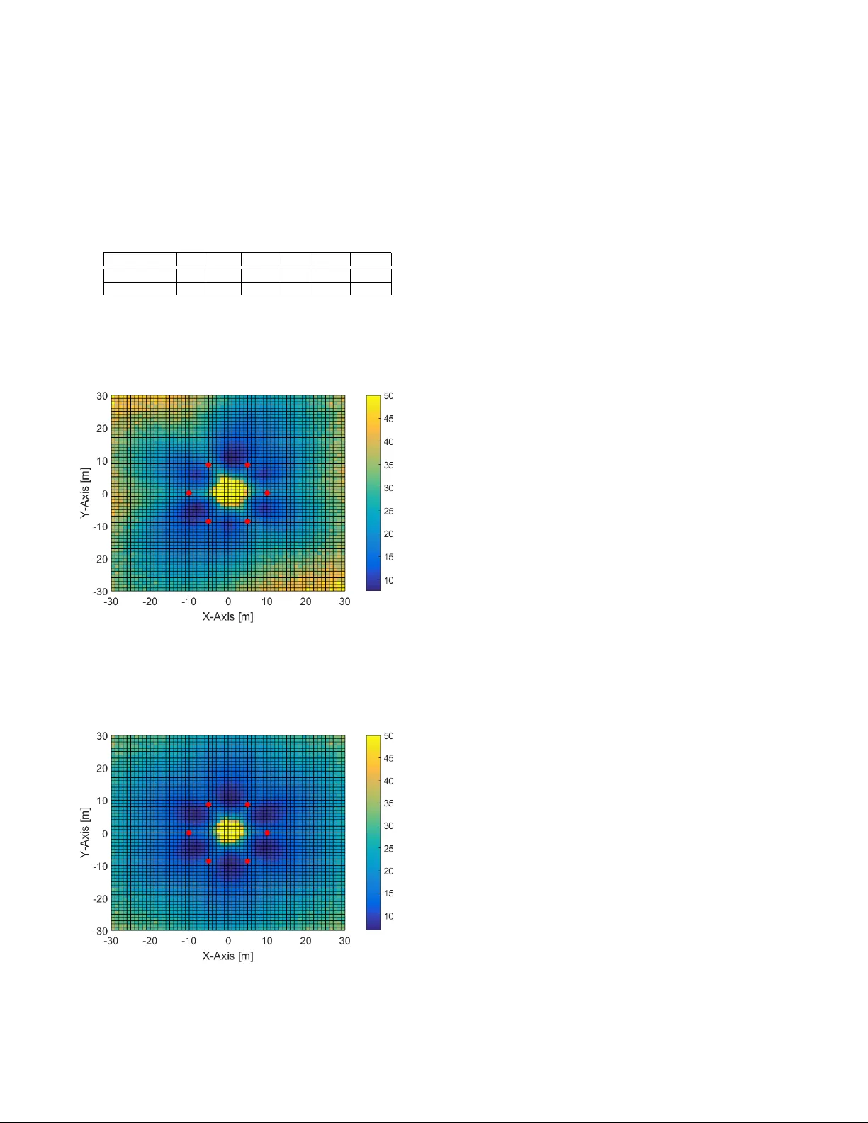
Impro v ed linear direct solution for asynchronous radio network localization (RNL) Juri Sidorenko, Norbert Scherer -Negenborn, Michael Arens, Eckart Michaelsen Fraunhofer Institute of Optronics, System T echnologies and Image Exploitation IOSB Gutleuthausstrasse 1, 76275 Ettlingen, Germany . Juri.Sidorenko@iosb .fraunhofer .de Abstract —In the field of localization the linear least squar e solution is fr equently used. This solution is compared to nonlinear solvers mor e effected by noise, but able to provide a position estimation without the knowledge of any starting condition. The linear least square solution is able to minimize Gaussian noise by solving an overdetermined equation with the Moore–P enrose pseudoin verse. Unfortunately this solution fails if it comes to non Gaussian noise. This publication presents a direct solution which is able to use pre-filtered data f or the LPM (RNL) equation. The used input for the linear position estimation will not be the raw data but ov er the time filtered data, for this reason this solution will be called direct solution. It will be shown that the presented symmetrical direct solution is superior to non symmetrical direct solution and especially to the not pr e-filtered linear least squar e solution. Keyw ords: direct solution, closed form, time of arrival, time diff erence of arrival, local position measurement I . I N T RO D U C T I O N Radio network-based localization is a radio wave-based positioning method, whereby a set of sensors at kno wn po- sitions (base stations) estimate the unknown sensor position (M). Range measurement can be accomplished using different principles, such as ’Round Trip T ime of Flight (R TT , R TT oF)’. W ith this approach, the base stations send the signal and it is sent back by M. This technique is v ery similar to radar , hence ev ery measurement can be referred to as ’Time Of Arri val (TO A) ’. Alternati vely , the base stations can be passiv e and only the M emits the signal, referred to as ’Local Position Measurement (LPM)’. The base stations have to be synchro- nized, which can be achie ved with a second transponder (T) at a known position. In contrast to the elliptical TDO A method [14], M and T do not communicate with each other , thus ev ery measurement has a time offset. The unknown sensor position can be estimated using the direct linear (closed loop) solution instead of T aylor-series expansion [5] or nonlinear solvers. The direct solution has the adv antage that no starting conditions are required compared to the nonlinear or T aylor solution. Ho wev er , e very real measurement is affected by noise, which is in the best Gaussian case. Unfortunately , reflections and other non-Gaussian disturbances can also be found in the measurements. The best approach is to filter this data before lateration, since ev en raw data with Gaussian noise can become non-Gaussian after a non-linear operation, caused by nonlinear optimization. This measurement principal requires data transformation to eliminate the time offset, filter the data and use it as an input for the linear solution. The Inmotiotec LPM system [7], [10] is an example of this kind of system and is able to provide an update rate of 1000 Hz with high three-dimensional position accuracy . I I . P R E V I O U S W O RK A linear algebraic solution (direct solution) is frequently used in the field of position estimation. One of those most commonly used is Bancroft’ s method [2], which is well analyzed and described in [1], [3]. Furthermore, it has been shown that the nonlinear solvers, such as the Gauss–Newton algorithm, provide more accurate solutions for overdetermined cases than the linear solution solved by the Moore–Penrose pseudoin verse [12]. In paper [11] we show an approach to using filtered measurements for the linear direct solution of the TO A-LPM equation. This solution is not symmetrical and less numerically stable, therefore an improved solution will be presented in this work. The Abatec LPM system itself is well described in [7], [10]. Pre vious publications about the Abatec LPM are mainly based on measurement principles [7], [10] and how the sensor data can be fused and filtered to detect outliers [4] and obtain the most accurate position [8] after multilateration. The latest publications on LPM focus on the numerical solvers. In general, LPM uses a Bancroft algorithm [9], [13], [4] to estimate the position of the transponder . I I I . M E T H O D O L O G Y The general LPM equation is R i = O + || M − B i || − || T − B i || (1) The pseudo range measurement (R), consists of the flight time between the first transponder and one base station subtracted from the reference transponder to the same base station. In this case, ev ery time offset (O=time offset*speed of light) remains the same for every base station at one measurement but changes rapidly over time. The Euclidian distance between the reference station equates with T indices eq.(2) and transponder with M indices eq.(3) to the base stations B with indices number ( i = 1 → n ) . || T − B i || = p ( x i − x T ) 2 + ( y i − y T ) 2 (2) || M − B i || = p ( x i − x M ) 2 + ( y i − y M ) 2 (3) The coordinates of the base stations and reference station are kno wn. Only the transponder position and the offset have to be estimated. A. Not symmetrical direct solution In contrast to approaches such as T aylor-series expansion [5], for which starting information for the unknown v ariables is required, it is possible to obtain the linear components x,y ,z of the transponder without deriv ation. The main LPM equation (1) can be simplified by adding the known reference transponder range to the measurement term R (pseudo range). L i = R i + || T − B i || (4) || M − B j || 2 − || M − B i || 2 = ( L j − O ) 2 − ( L i − O ) 2 (5) The known quadratic terms of the transponder are elimi- nated, hence the linear solution for the transponder position at the known base station and reference station position is ( − → B i − − → B j ) · − → M − ( L i − L j ) · O = = 1 2 (( − → B i 2 − − → B j 2 ) − ( L 2 i − L 2 j )) (6) W ith: − → M =  x M y M  − → B =  x B y B  In [11] it is shown that the linear solution for the LPM is highly affected by noise. The measurement L 1 cannot be filtered as the time offset change with respect to time is 1000 times higher than the range change itself. Therefore, the offset is eliminated by subtracting one base station measurement from the other ( L i − L j ) . In the next step this data is filtered ov er time. At this point it does not matter what kind of filter is used, it is only important that filtering takes place before position estimation and that the filter uses the measurement difference ( L i − L j ) as an input. For the following calculations we only assume that for every measurement we already hav e difference ( L i − L j ) the filtered v alues F ( L i − L j ) , the main aim is to use the filtered values instead of the measurement differences between the base stations. The ( L 2 i − L 2 j ) term is nonlinear but the filtered values consist of the linear difference between the measurement ranges. One solution to using the filtered v alues would be to make ev ery base station dependent on the same measurement error term α i. Every measurement is corrupted by the measurement error α i, hence the real measurement can be written as L = ˜ L i + α . The connection between the measurement errors α i and α j can be found if the unfiltered measurement difference (( L i + α i ) − ( L j + α j )) is subtracted from the filtered values F ( L i − L j ) . F ij = (( ˜ L i + α i ) − ( ˜ L j + α j )) − F ( L i − L j ) (7) ( ˜ L i − ˜ L j ) ≈ F ( L i − L j ) (8) The assumption that the noise can be neglected after the filtering, this leads to the term F ij being the dif ference between the noises of both signals. F ij = α i − α j (9) α j = − F ij + α i (10) The measurement error α j is replaced by − F ij + α i ( − → B i − − → B j ) · − → M − ( ˜ L i − ˜ L j + F ij ) · O = = 1 2 (( − → B i 2 − − → B j 2 ) − ˜ L i 2 − ˜ L j 2 − F 2 ij + + 2 · α k ( ˜ L i − ˜ L j + F ij )) (11) It can be observed that the time offset Z, depends on the same parameter as the measurement error ( − → B i − − → B j ) · − → M − ( ˜ L i − ˜ L j + F ij ) · ( O + α k ) = = 1 2 (( − → B i 2 − − → B j 2 ) − ˜ L i 2 − ˜ L j 2 − F 2 ij ) (12) W ith at least four base stations, the unknown coordinates of the transponder can be estimated. W ith the filtered v alues the linear direct solution provides better results, than with the unfiltered equation. Ax = b (13) This equation can be solved as:   x M y M O   = ( A T ∗ A ) − 1 A T ∗ b (14) B. Symmetrical direct solution The main disadv antage of the pre vious equation is that ev ery base station measurement depends on one and the same base station, hence the solution is not symmetrical. Therefore, a more rob ust approach whereby e very base station is used will be presented in the next part. In contrast to the solution presented in 3.1, the nonlinear dif ference between the measurements will be rewritten as. ( L 2 i − L 2 j ) = ( L i − L j ) · ( L i + L j ) (15) This leads to the term ( − → B i − − → B j ) · − → M − ( L i − L j ) · ( O − L i + L j 2 ) = = 1 2 ( − → B i 2 − − → B j 2 ) (16) The dif ference between two measurements ∆ ij can be re- placed by results of the filter . ∆ ij = ( L i − L j ) (17) Filtering uses the differences between two measurements, as offset O is equal for the same measurement for ev ery base station. Therefore, e very measurement dif ference ( L − L j ) can be replaced by the filtered v alues. Only the sum between two measurements ( L 1 + L j ) is unknown. ( − → B i − − → B j ) · − → M − ∆ i,j · ( O − L i + L j 2 ) = 1 2 ( − → B i 2 − − → B j 2 ) (18) ∆ j i = − ∆ ij , ∆ ii = 0 (19) In the follo wing example, it will be sho wn how the sum of two measurements ( L i + L j ) is represented by the Differences of two measurements ( L i − L j ) . Symmetrical dir ect solution: Example with 5 base stations For five base stations the filtered measurement differences required are B S 1 − j B S 2 − j B S 3 − j B S 4 − j j=2 1-2 2-3 3-4 4-5 j=3 1-3 2-4 3-5 j=4 1-4 2-5 j=5 1-5 The sum of measurements L i + L j for five base stations can be represented by the filtered measurement differences: L 1 + L 3 = ( L 1 + L 2 ) − ( ∆ 23 ) L 1 + L 4 = ( L 1 + L 2 ) − ( ∆ 24 ) L 1 + L 5 = ( L 1 + L 2 ) − ( ∆ 25 ) L 2 + L 3 = ( L 1 + L 2 ) − ( ∆ 13 ) L 2 + L 4 = ( L 1 + L 2 ) − ( ∆ 14 ) L 2 + L 5 = ( L 1 + L 2 ) − ( ∆ 15 ) L 3 + L 4 = ( L 1 + L 2 ) − ( ∆ 13 ) − ( ∆ 24 ) L 3 + L 5 = ( L 1 + L 2 ) − ( ∆ 13 ) − ( ∆ 25 ) L 4 + L 5 = ( L 1 + L 2 ) − ( ∆ 25 ) − ( ∆ 34 ) Now ev ery base station depents on the unkown sum com- ponent ( L 1 + L 2 ) . Insted of ( L 1 + L 2 ) it is also possible to use any combination of ( L i + L j ). Our aim is to make the equation equally dependent on all the base stations and not only on fixed base station combinations ( L i + L j ). For this reason, the sum ( L i + L j ) between two base stations will be replaced by the sum of all base stations. If we stay by the example with five base stations, the sum S would be. S = n X i =1 L i (20) This unko wn sum S should now fit for ev ery ( L i + L j ). If the indizes are i=1 and j=2, the sum S need to be transfomred in such a way that L 3 + L 4 + L 5 are eliminated by only using the differences between the L i and L j . For L 1 + L 2 6 = S + ( L 1 − L 3 ) + ( L 1 − L 4 ) + ( L 1 − L 5 ) (21) the components L 3 , L 4 and L 5 are eliminated but no w L 1 is represented four times instead of once. If the equation is changed to L 1 + L 2 6 = S + ( L 1 − L 3 ) + ( L 1 − L 4 ) + ( L 1 − L 5 )+ + ( L 2 − L 3 ) + ( L 2 − L 4 ) + ( L 2 − L 5 ) (22) the measurements L 1 and L 2 are now overrepresented four times and L 3 , L 4 and L 5 are overrepresented twice. By multiplying the measurement differences by 0.5 and adding them to the sum S, the L 3 , L 4 and L 5 are eliminated but L 1 and L 2 now have the factor 5/2 instead of one. The numerator represents the number of base stations used, in this example fiv e. The term ( L i + L − j ) can now be expressed as L 1 + L 2 = 2 5 · ( S + 1 2 (( L 1 − L 3 ) + ( L 1 − L 4 ) + ( L 1 − L 5 )+ + ( L 2 − L 3 ) + ( L 2 − L 4 ) + ( L 2 − L 5 ))) (23) The general equation for ev ery L i + L j becomes L i + L j = 2 n · S + 1 n · 2 · ( X k 6 = i,j ( ∆ ik ) + X k 6 = i,j ( ∆ j k )) (24) with the variable n, which stands for the number of base stations. The sum of the measurements between two base stations can no w be replaced by the following term, whereby ev ery other base station is used equally . L i + L j 2 = 1 n · S + 1 n · 2 · ( X k 6 = i,j ∆ ik + X k 6 = i,j ∆ j k ) (25) The final symmetrical direct solution, with the unko wn variables x M T , y M T , z M T , O and S equates: ( − → B i − − → B j ) · − → M − ∆ i,j · ( O − 1 n · S ) = = 1 2 ( − → B i 2 − − → B j 2 ) − ∆ i,j · 1 2 · n · ( X k 6 = i,j ∆ ik + X k 6 = i,j ∆ j k ) (26) I V . R E S U L T S In the following two methods (symmetrical and non- symmetrical) filtering the direct solution will be compared. The fi ve base station positions are located on a circle with a radius of 10 metres and the transponder position measurement is calculated for every metre in the 60 m 2 square area. Fur- thermore, the measurements ha ve been corrupted by Gaussian noise with a variance of 0 . 064 m 2 . This noise represents the filtering error not the measurement noise. Base station 1 2 3 4 5 6 X-Axis [m] 10 5 -5 -10 -5 5 Y -Axis [m] 0 8.66 8.66 0 -8.66 -8.66 T ABLE I B A S E S TA T I O N P O SI T I ON Fig. 1. Matrix condition with BS 1 as reference. Colours from yello w to blue: condition at the specific position. The red dots: base station positions.. Fig. 2. Matrix condition symmetric approach. Colours from yello w to blue: condition at the specific position. The red dots: base station positions.. The position error of the previous method is subtracted from the new one at any position in the square area. Positive error differences indicate that the error with the second method is smaller . On the other hand, negativ e error dif ference shows that the error with the second approach is higher compared to the non-symmetrical solution. In the set-up presented, 56.11% hav e a positive error difference and 43.88% a negati ve one. Therefore, the second approach is 13% superior to the first one. In some test scenarios, where the geometrical constellation of the base stations is difficult for the lateration of the transponder position, the difference between the non-symmetrical and symmetrical approach increases by 30%. The first approach (non-symmetrical) always uses the same base station (base station one) from which the others are subtracted. If this transformation station is selected by the best condition of the coefficient matrix || A || ∗ || A − 1 || , the error difference between the new and previous approach is almost always a value between 50.44 % and 49.55 %. The increase in noise when selecting dif ficult geometrical constellations of the base stations leads to a higher dif ference between the symmetrical and non-symmetrical approach, with better results for the symmetrical approach. The condition of the coef ficient matrix at different transponder positions can be seen in figure 1 and 2. It can be observed that the coef ficient matrix condition with the previous method, figure 1 is not symmetrical compared to the new approach figure 2. Base station selection with the best condition slightly changes the results but still underlies the symmetrical approach. The condition appears to be best in the area between the base stations. This is not always the case and depends on the base station constellation. V . C O N C L U S I O N ’LPM’ is a nonlinear offset corrupted equation, whereby any transformation to a linear solution leads to a high noise impact on the outcome. W e present a new numerically more stable direct solution, which is able to work with prefiltered data. In contrast to a non-filtered linear least square solution, this filtered direct solution is statically not correct, as not the data corrupted by Gaussian noise is used b ut the output of the filter . The results of this filtered direct solution are less influenced by the noise and therefore more suitable for use as starting values for the nonlinear solver . Furthermore, the symmetrical approach does not require a specific base station that is used for filtering, but instead all base stations play an equal part in finding a solution. The results of the new approach are at least 10 % better , compared to approaches whereby only the same base station is used. The best result for the first solution appears if the reference station that causes the best condition matrix is selected. In the new solution, there is no need to find the base station which causes the best matrix condition since every base station is used equally . Especially when the noise increases or the geometrical set-up is unfa vourable, the results of the symmetrical approach are superior to its non- symmetrical counterpart. R E F E R E N C E S [1] J. S. Abel and J. W . Chaffee. Existence and uniqueness of gps solutions. IEEE Tr ansactions on Aer ospace and Electr onic Systems , 27(6):952– 956, Nov 1991. [2] S. Bancroft. An algebraic solution of the gps equations. IEEE T ransactions on Aer ospace and Electr onic Systems , AES-21(1):56–59, Jan 1985. [3] J. Chaffee and J. Abel. On the exact solutions of pseudorange equations. IEEE T ransactions on Aer ospace and Electronic Systems , 30(4):1021– 1030, Oct 1994. [4] R. Pfeil et al. Distributed fault detection for precise and robust local positioning. In In Pr oceedings of the 13th IAIN W orld Congr ess and Exhibition , 2009. [5] W . H. FOY . Position-location solutions by taylor-series estimation. IEEE T ransactions on Aer ospace and Electr onic Systems , AES-12(2):187–194, March 1976. [6] R. Pfeil, S. Schuster, P . Scherz, A. Stelzer, and G. Stelzhammer . A robust position estimation algorithm for a local positioning measurement system. In W ireless Sensing, Local P ositioning, and RFID, 2009. IMWS 2009. IEEE MTT -S International Microwave W orkshop on , pages 1–4, Sept 2009. [7] K. Pourvoyeur , A. Stelzer, Alexander Fischer, and G. Gassenbauer . Adaptation of a 3-D local position measurement system for 1-D ap- plications. In Radar Confer ence, 2005. EURAD 2005. Eur opean , pages 343–346, Oct 2005. [8] K. Pourvoyeur , A. Stelzer, T . Gahleitner , S. Schuster , and G. Gassen- bauer . Effects of motion models and sensor data on the accuracy of the LPM positioning system. In Information Fusion, 2006 9th International Confer ence on , pages 1–7, July 2006. [9] K. Pourvoyeur , A. Stelzer , and G. Gassenbauer . Position estimation tech- niques for the local position measurement system LPM. In Micr owave Confer ence, 2006. APMC 2006. Asia-P acific , pages 1509–1514, Dec 2006. [10] A. Resch, R. Pfeil, M. W egener , and A. Stelzer. Review of the LPM local positioning measurement system. In Localization and GNSS (ICL- GNSS), 2012 International Conference on , pages 1–5, June 2012. [11] J. Sidorenko, N. Scherer-Negenborn, M. Arens, and E. Michaelsen. Multilateration of the local position measurement. In 2016 International Confer ence on Indoor P ositioning and Indoor Navigation (IPIN) , pages 1–8, Oct 2016. [12] N. Sirola. Closed-form algorithms in mobile positioning: Myths and misconceptions. In 2010 7th W orkshop on P ositioning, Navigation and Communication , pages 38–44, March 2010. [13] A. Stelzer, K. Pourv oyeur , and A. Fischer . Concept and application of lpm - a nov el 3-d local position measurement system. IEEE T ransactions on Microwave Theory and T ec hniques , 52(12):2664–2669, Dec 2004. [14] Y . Zhou, C. L. Law , Y . L. Guan, and F . Chin. Indoor elliptical localization based on asynchronous uwb range measurement. IEEE T ransactions on Instrumentation and Measur ement , 60(1):248–257, Jan 2011.