Fundamental Limits on Data Acquisition: Trade-offs between Sample Complexity and Query Difficulty

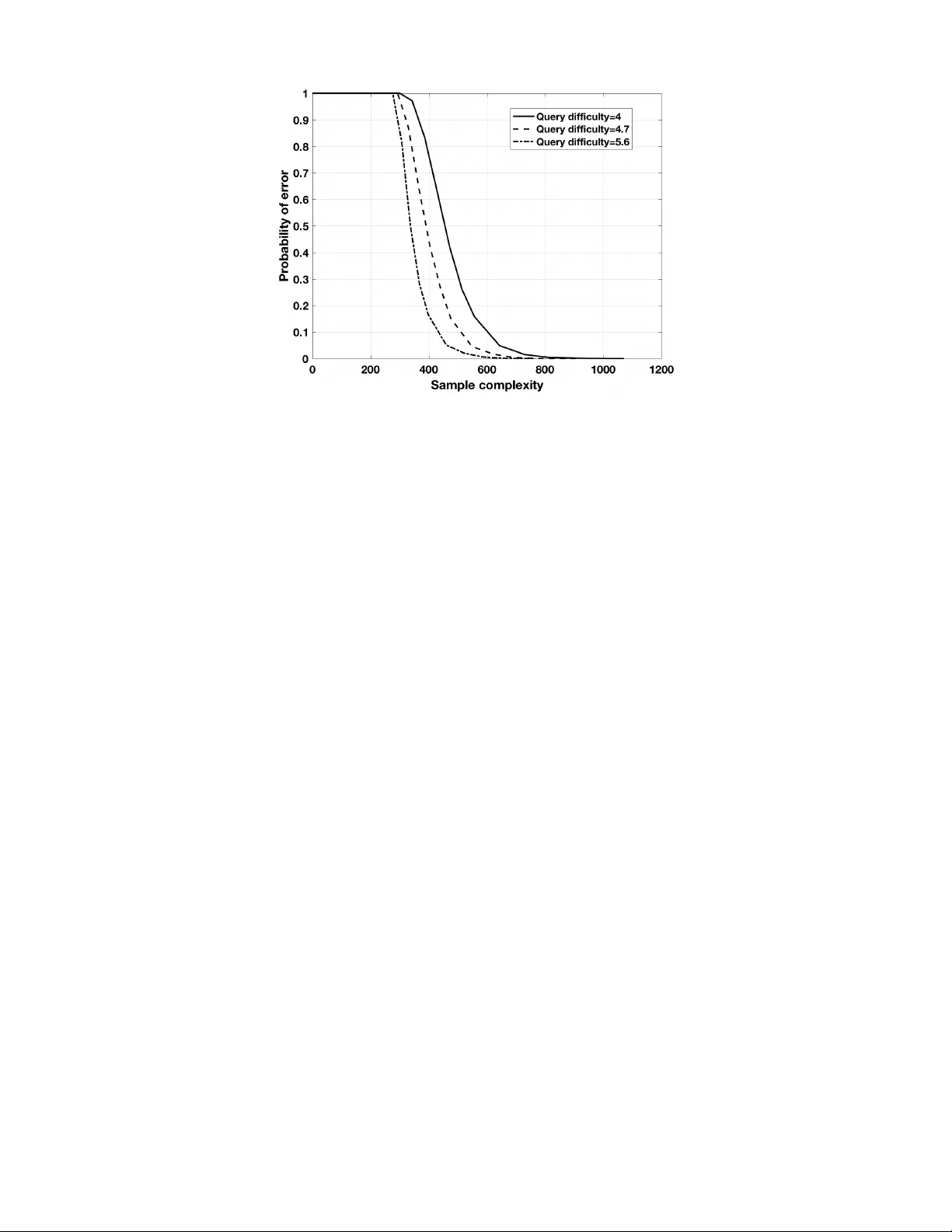
1 Fundamental Limits on Data Acquisition: T rade-of fs between Sample Comple xity and Query Dif ficulty Hye W on Chung ∗ , Ji Oon Lee, and Alfred O. Hero Abstract W e consider query-based data acquisition and the corresponding information recovery problem, where the goal is to recov er k binary variables (information bits) from parity measurements of those variables. The queries and the corresponding parity measurements are designed using the encoding rule of Fountain codes. By using Fountain codes, we can design potentially limitless number of queries, and corresponding parity measurements, and guarantee that the original k information bits can be recov ered with high probability from any sufficiently lar ge set of measurements of size n . In the query design, the av erage number of information bits that is associated with one parity measurement is called query dif ficulty ( ¯ d ) and the minimum number of measurements required to recover the k information bits for a fixed ¯ d is called sample complexity ( n ). W e analyze the fundamental trade-of fs between the query difficulty and the sample complexity , and show that the sample complexity of n = c max { k , ( k log k ) / ¯ d } for some constant c > 0 is necessary and sufficient to recover k information bits with high probability as k → ∞ . Index T erms Sample complexity , query difficulty , Fountain codes, Soliton distribution, crowdsourcing. I . I N T R O D U C T I O N Query-based data acquisition arises in diverse applications including: crowdsourcing [1], [2]; activ e learning [3], [4]; experimental design [5], [6]; and community recov ery or clustering in graphs [7], [8]. In these applications, query-based data acquisition can be modeled as a 20 questions problem [9] between an oracle (or oracles) and a player where the oracle knows the values of information bits that the player aims to recover , while the player designs queries to the oracle and receives answers from the oracle. In this paper , we consider query-based data acquisition with the goal of recovering the v alues of k variables ( x 1 , . . . , x k ) (information bits). When we assume that the v ariables and the answers (measurements) are binary , we can consider a parity check sum as a type of measurement, which corresponds to exclusi ve or (XOR or modulo 2 sum) of some subset of the information bits. Querying parity symbols of the information bits generalizes the 20 questions model of [9], [10]. This generalization is the focus of this paper and has a wide range of applications, in particular to crowdsourcing systems [1]. Consider a crowdsourcing system consisting of a number of workers and a particular task that they are expected to work on. Assume that the task is to classify a collection of k images into two exclusi ve groups, e.g., whether or not an image is suitable for children. A worker (oracle) in the system is giv en a query about some subset of the images and asked to provide a binary answer re garding those images. Assume that the worker can skip the query if the worker is unsure of the answer . The probability that one worker skips a query is unkno wn at the stage of query design and it can be different for each of the work ers in the system, depending on their abilities or ef forts. Therefore, from the query designer’ s point of view , it is natural to assume that only a random subset of the designed queries will be answered by the workers in the crowdsourcing system. The query designer’ s objectiv e is to design queries such that when the receiv ed number of answers exceeds some threshold, regardless of which subset of the answers was collected, the original k binary bits can be recovered with high probability . In this paper we show that Fountain codes [11] are naturally suited to this crowdsourcing query design problem. Fountain codes are a type of forward error correcting codes suitable for binary erasure channels (BEC) with unkno wn erasure probabilities. This type of codes has been the subject of much research for reliable internet packet transmissions when the packets transmitted from the source are randomly lost before they arrive at the destination. Hye W on Chung ∗ (hwchung@kaist.ac.kr) is with the School of Electrical Engineering at KAIST in South Korea. Ji Oon Lee (jioon.lee@kaist.edu) is with the Department of Mathematical Sciences at KAIST in South Korea. Alfred O. Hero (hero@eecs.umich.edu) is with the Department of EECS at the Univ ersity of Michigan. This work was partially supported by National Research Foundation of K orea under grant number 2017R1E1A1A01076340, and by United States Army Research Office under grant W911NF-15-1-0479. 2 For k input symbols ( x 1 , x 2 , . . . , x k ) , Fountain codes produce a potentially limitless number of parity measurements, which are also called output symbols. By using well-designed F ountain codes, one can guarantee that, giv en any set of output symbols of size k (1 + δ ) with small ov erhead δ > 0 , the input symbols can be reco vered with high probability . Examples of Fountain codes are L T -codes [12] and Raptor codes [13]. By using these Fountain codes, we can design potentially limitless number of queries (and corresponding parity measurements) with the desired properties suitable for the crowdsourcing example. Ho wev er, the Fountain code framework must be extended in order to account for the worker’ s limited capacity to answer dif ficult queries. The query difficulty is defined as the average number of input symbols required to compute a single parity measurement. The query difficulty is related to the encoding complexity for one-stage encoding, but it is dif ferent from the encoding complexity when the encoding is done in multiple stages. The query dif ficulty represents the number of input symbols on av erage the worker must kno w to calculate one parity measurement. Depending on the query difficulty , the number of answers (parity measurements) required to recover k input symbols may vary greatly . W e call the minimum number of measurements required to recov er k input symbols the sample complexity . The sample comple xity is a function of the query dif ficulty as well as the number k of input symbols to be recovered. Let us consider two extreme cases. First, consider the case when the query difficulty is equal to 1. More specifically , we assume that each query asks the v alue of only one variable in ( x 1 , x 2 , . . . , x k ) at a time. Since it is not known which of the queries would be answered by the workers at the stage of query design, a set of queries is designed by uniformly and randomly picking one variable in ( x 1 , x 2 , . . . , x k ) at a time. For such querying scenarios, with randomly selected n measurements, in order to recover the k information bits with error probability less than 1 /k u for some constant u > 0 , the required number n of queries scales as k log k . On the other hand, when each query is designed to generate a parity measurement of randomly selected k/ 2 bits at a time, the required number n of measurements is only k + c log k for some constant c > 0 [13]. Therefore, in these two extreme cases, we can observe that when the query difficulty is equal to 1, the sample complexity scales as k log k , whereas for the query dif ficulty of order k the sample complexity scales as k . Then the question is ho w the sample complexity scales as the query difficulty increases from 1 to Θ( k ) . In this paper , we aim to analyze the fundamental trade-offs between the sample complexity and the query dif ficulty in recov ering k information bits. There have been papers that hav e analyzed such trade-offs when it is assumed that the parity measurements in volv e only a fixed number 1 ≤ d ≤ k of input symbols. In [14], the case of pairwise measurements ( d = 2 ) was considered and in [15], a general integer 1 ≤ d ≤ k was considered. Note that there are a total of  k d  possible parity measurements for a fixed d . In both papers, it was assumed that each measurement is independently observed with probability p obs . It was shown that the number n of measurements to recover k input symbols with high probability scales as n = p obs  k d  = c max { k , ( k log k ) /d } for some constant c > 0 . In this paper , we generalize the work in [15] by not fixing the number d but instead allo wing that the number d follows a distrib ution (Ω 0 , Ω 1 , . . . , Ω k ) where Ω d denotes the probability that the v alue d is chosen, where P k d =0 Ω d = 1 . W e consider the average query dif ficulty ¯ d = P k d =0 d Ω d and analyze the sample complexity n as a function of the query dif ficulty ¯ d and the number k of input symbols. By assuming that d follows the prescribed distribution, we can generate potentially limitless parity measurements by using the encoding rule employed by Fountain codes; guaranteeing that for any set of fixed number of measurements it is possible to recover the k input symbols with high probability . This frame work is thus more suitable for the situations where the parity measurements are erased with arbitrary (unknown) probabilities and thus it is required to have the ability to generate potentially limitless number of queries and corresponding parity measurements. For the pre vious framew orks in [14], [15], the maximum number of parity measurements is restricted to  k d  for a fixed d . Our main contribution in this paper is to specify the fundamental trade-offs between the sample complexity ( n ) and the query difficulty ( ¯ d ) in this generalized measurement model. W e sho w that the sample complexity n necessary and sufficient to recover k input symbols with high probability scales as n = c · max  k , ( k log k ) / ¯ d  (1) for some constant c > 0 . Note that for ¯ d = O (log k ) , the sample complexity n is in versely proportional to the query dif ficulty ¯ d . In particular , when query difficulty ¯ d = Θ(1) , the sample complexity scales as k log k , whereas when ¯ d = Θ(log k ) , the sample complexity scales as k . 3 The rest of this paper is organized as follo ws. In Section II, we explain the encoding rule of Fountain codes (ho w to generate potentially limitless number of parity measurements) and state the main problem of this paper . In Section III, we provide the main results, showing the fundamental trade-offs between the sample comple xity and the query difficulty . In Section IV, we prov e the main theorem. More technical details for the proof are presented in Appendices. In Section V, some simulation results are pro vided, which further support our theoretical results. In Section VI, we provide conclusions and discuss possible future research directions. A. Notations W e use the notation ⊕ for XOR of binary variables, i.e., for a, b ∈ { 0 , 1 } , a ⊕ b = 0 iff a = b and a ⊕ b = 1 iff a 6 = b . W e denote by e j the k -dimensional unit vector with its j -th element equal to 1. For a vector x , k x k 1 denotes the number of 1 ’ s in the vector x . F or vectors x and y , the inner product between x and y is denoted by x · y . For two integers α and β , we use the notation α ≡ β to indicate that mo d( α, 2) = mo d( β , 2) . For two vectors x = ( x 1 , x 2 , . . . , x k ) and y = ( y 1 , y 2 , . . . , y k ) , when we write x ≡ y , it means that mo d( x i , 2) = mo d( y i , 2) for all i ∈ { 1 , 2 , . . . , k } . W e use the O ( · ) and Θ( · ) notations to describe the asymptotics of real sequences { a k } and { b k } : a k = O ( b k ) implies that a k ≤ M b k for some positi ve real number M for all k ≥ k 0 ; a k = Θ( b k ) implies that a k ≤ M b k and a k ≥ M 0 b k for some positiv e real numbers M and M 0 for all k ≥ k 0 0 . The logarithmic function log is with base e . I I . M O D E L A N D P RO B L E M S T A T E M E N T Consider a k -dimensional binary random vector x = ( X 1 , X 2 , . . . , X k ) T , which is uniformly and randomly distributed ov er { 0 , 1 } k . W e call X 1 , X 2 , . . . , X k the input symbols. W e aim to learn the v alues of ( X 1 , X 2 , . . . , X k ) by observing a total of n parity measurements of different subsets of those k bits. Consider k -dimensional binary vectors v i = ( v i 1 , v i 2 , . . . , v ik ) , i = 1 , . . . , n . The parity measurement associated with the vector v i is defined by Y i = mo d   k X j =1 v ij X j , 2   = v i 1 X 1 ⊕ · · · ⊕ v ik X k , (2) for i = 1 , . . . , n . W e call such parity measurements ( Y 1 , Y 2 , . . . , Y n ) the output symbols. Each v i ∈ { 0 , 1 } k determines which subset of ( X 1 , X 2 , . . . , X k ) is to be picked in calculating the i -th parity measurement. The process of designing { v i } is called query design or encoding. W e use Fountain codes, also known as erasure rateless codes, for the encoding. Let (Ω 0 , Ω 1 , . . . , Ω k ) be a distribution on { 0 , 1 , . . . , k } where Ω d denotes the probability that the value d is chosen and P k d =0 Ω d = 1 . In the encoding of F ountain codes, each v ector v i is generated independently and randomly by first sampling a weight d ∈ { 0 , 1 , . . . , k } from the distribution (Ω 0 , . . . , Ω k ) and then selecting a k -dimension vector of weight d uniformly at random from all the vectors of { 0 , 1 } k with weight d . Consider an arbitrary set of n output symbols ( Y 1 , . . . , Y n ) generated by the above encoding rule. The relationship between the k input symbols and the n output symbols can be depicted by a bipartite graph with k input nodes on one side and n output nodes on the other side as shown in Fig 1. Denote by ¯ d the av erage degree of the output nodes, ¯ d = k X d =1 d · Ω d . (3) This number ¯ d indicates the average number of input symbols in volved in one parity measurement (output symbol) and is related to the dif ficulty in calculating one parity measurement. W e call this number query dif ficulty . The process of recovering the k input symbols from the n output symbols is called information recov ery or decoding. Denote by ˆ x ( Y k 1 ) the estimate of x gi ven Y n 1 and define the probability of error as P ( k ) e = min ˆ x ( · ) Pr( ˆ x ( Y k 1 ) 6 = x ) . (4) W ith the proper choice of the distribution (Ω 0 , . . . , Ω k ) , the Fountain codes guarantee that P ( k ) e → 0 as k → ∞ with n larger than some threshold. The minimum number of n required to guarantee P ( k ) e → 0 as k → ∞ , minimized ov er all (Ω 0 , . . . , Ω k ) for a fixed k and ¯ d , is called sample comple xity . W e aim to find the fundamental limits on n to guarantee reliable information reco very of k input symbols for a fix ed query difficulty ¯ d . 4 . . . x 1 x 2 x 3 x 4 x 5 x 6 y 1 y 2 y 3 y 4 y 5 y 6 y 7 Input nodes Output nodes . . . y n x k Fig. 1. Bipartite graph between input nodes and output nodes. I I I . M A I N R E S U LT S : F U N DA M E N TA L T R A D E - O FF S B E T W E E N S A M P L E C O M P L E X I T Y A N D Q U E RY D I FFI C U L T Y In this section, we state our main results that the sample complexity n that is necessary and sufficient to make P ( k ) e → 0 as k → ∞ scales in terms of k and ¯ d as n = c · max { k , ( k log k ) / ¯ d } for some constant c > 0 independent of k and ¯ d , when the parity measurements are generated by the encoding rule of Fountain codes as explained in Section II. W e first state the well-kno wn lower bound on the sample complexity n of F ountain codes presented in [13]. Pr oposition 1: T o r eliably r ecover k input symbols with P ( k ) e ≤ 1 /k u for some constant u > 0 fr om parity measur ements g enerated by F ountain codes, it is necessary that n ≥ c l max  k , k log k ¯ d  (5) for some constant c l > 0 . Pr oof: Sho wing the first condition n ≥ c l k is straightforward. Each output symbol Y i = mo d  P k j =1 v ij X j , 2  represents a linear equation of k unknown input symbols ( X 1 , X 2 , . . . , X k ) . Since there are k unknowns, it is necessary to have at least n = k linear equations to solve this linear system reliably . The second condition n ≥ ( c l k log k ) / ¯ d is from a property of random graphs. In the bipartite graph between input nodes and output nodes, we say that an input node is isolated if it is not connected to any of the output nodes. W e analyze the probability that an input node is isolated when the edges are designed by the encoding rule of F ountain codes. The error probability P ( k ) e is bounded below by the probability that an input node is isolated, since when an input node is isolated the decoding error happens. Consider an output node with degree d . The probability that an input node is not connected to this output node of de gree d equals 1 − d/k . Since an output node has de gree d with probability Ω d , the probability that an input node is not connected to an output node equals k X d =0 Ω d (1 − d/k ) = 1 − ¯ d/k . (6) Since there are n output nodes and these output nodes are sampled independently , the probability that an input node is isolated (not connected to any of those output nodes) equals  1 − ¯ d k  n . (7) By the mean value theorem, we can sho w that (1 − ¯ d/k ) n ≥ e − α/ (1 − α/n ) where α = n ¯ d/k . Since the decoding error probability P ( k ) e is lower bounded by the probability that an input node is isolated, to satisfy P ( k ) e ≤ 1 /k u 5 for some constant u > 0 , it is necessary that e − α/ (1 − α/n ) ≤ 1 /k u , which is equi valent to α ≥ log k · u 1 + ( u log k ) /n ≥ log k · u 1 + ( u log k ) /k ≥ log k · u 1 + ( u log 3) / 3 ≥ c l log k (8) for some constant c l > 0 . By plugging in α = n ¯ d/k , we get n ¯ d ≥ c l k log k . (9) The main contribution of this paper is showing that the bound in (5) is indeed achiev able (up to constant scaling) by properly designed Fountain codes for any ¯ d from Θ(1) to Θ(log k ) . W e provide a particular output degree distribution (Ω 0 , Ω 1 , . . . , Ω k ) for which we can control the query difficulty ¯ d from Θ(1) to Θ(log k ) and sho w that it is possible to reliably reco ver k information bits with sample complexity obeying n = c u max  k , k log k ¯ d  (10) for some constant c u > 0 . Therefore, by combining (10) with (5), we conclude that n = c · max { k , ( k log k ) / ¯ d } is necessary and sufficient for reliable recovery of k information bits when ¯ d is the a verage query dif ficulty . Suppose that the la w of Ω d is giv en by an ideal Soliton distrib ution Ω d =      1 D if d = 1 1 d ( d − 1) if 2 ≤ d ≤ D 0 if d > D or d = 0 , (11) for some D ∈ { 2 , 3 , . . . , k } . Here, for simplicity , we assume that k ≥ 3 . Note that the query dif ficulty scales as log D since log( D + 1) < ¯ d = 1 D + D X d =2 1 d − 1 = D X d =1 1 d < log D + 1 . Therefore, as D increases from 2 to k , the query dif ficulty ¯ d scales from log 3 to log k . Theor em 1: F or the Soliton distribution (11) with D ∈ { 2 , 3 , . . . , k } , the k input symbols can be r eliably r ecover ed, i.e., P ( k ) e → 0 as k → ∞ , with sample complexity n = c u · max  k , k log k ¯ d  (12) for some constant c u > 0 . The proof of Theorem 1 will be presented in Section IV. Theorem 1 states that for query difficulty ¯ d = O (log k ) , the sample complexity n to reliably recover k input symbols is inv ersely proportional to the query difficulty ¯ d . When the query difficulty does not increase in k , i.e., ¯ d = Θ(1) , it is necessary and sufficient to hav e n = Θ( k log k ) to reliably recover the k information bits. In this regime, the ratio between k and n con verges to 0 as k → ∞ . On the other hand, when we increase the query dif ficulty to ¯ d = Θ(log k ) , it is enough to hav e n = Θ( k ) samples, which results in a positiv e limit of k /n as k → ∞ . When ¯ d  log k , increasing the query dif ficulty no longer helps in reducing the sample complexity . By using the Soliton distribution (11) and the encoding rule of Fountain codes, we can design potentially limitless number of queries about ( x 1 , x 2 , . . . , x k ) and the corresponding parity measurements. Theorem 1 shows that with any set of measurements of size n no larger than (12), we can reliably recov er the k information bits as k → ∞ . Moreov er , this sample size is optimal up to constants as shown by Proposition 1. Thus, our results provide the optimal query design strategy for reliable information recovery from an arbitrary set of parity measurements, optimal in terms of the sample comple xity (up to constants) for a fixed query difficulty . 6 I V . P RO O F O F T H E O R E M 1 In this section, we prov e Theorem 1 by providing an upper bound on P ( k ) e and sho wing that the sample complexity n suf ficient to make this upper bound conv erge to 0 as k → ∞ is equal to c u · max { k , ( k log k ) / ¯ d } for some constant c u > 0 . Consider P ( k ) e defined in (4). The optimal decoding rule ˆ x ( · ) that minimizes the probability of error is the maximum likelihood (ML) decoding for the uniformly distributed input symbols. Assume that we collect n parity measurements ( Y 1 , . . . , Y n ) each of which equals Y i = mo d  P n j =1 v ij X j , 2  . Consider a matrix A whose i -th row is v i = ( v i 1 , v i 2 , . . . , v ik ) , i.e., A := [ v 1 ; v 2 ; . . . ; v n ] . (13) W e call A a sampling matrix. Giv en ( Y 1 , . . . , Y n ) and the sampling matrix A , the ML decoding rule finds x = ( X 1 , X 2 , . . . , X k ) T ∈ { 0 , 1 } k such that A x ≡ ( Y 1 , Y 2 , . . . , Y n ) T . (14) If there is a unique solution x ∈ { 0 , 1 } k for this linear system, then it is claimed that ˆ x ( Y k 1 ) = x . If there is more than one x satisfying this linear system, then an error is declared. The probability of error is thus equal to P ( k ) e = X x ∈{ 0 , 1 } k 1 2 k Pr( ∃ x 0 6 = x such that A x 0 ≡ A x ) . (15) Due to symmetry , the probabilities Pr( ∃ x 0 6 = x such that A x 0 ≡ A x ) are equal for e very x ∈ { 0 , 1 } k . Thus, we focus on the case where x is the vector of all zeros and consider P ( k ) e = Pr( ∃ x 0 6 = 0 such that A x 0 ≡ 0 ) . (16) By using the union bound, it can be shown that P ( k ) e ≤ X x 0 6 = 0 Pr( A x 0 ≡ 0 ) = k X s =1 X k x 0 k 1 = s Pr( A x 0 ≡ 0 ) = k X s =1  k s  Pr A s X i =1 e i ! ≡ 0 ! (17) where e i is the i -th standard unit vector . The last equality follows from the symmetry of the sampling matrix A . Since all the output samples are generated independently by the identically distributed v i ’ s, each of which has weight d with probability Ω d , P ( k ) e ≤ k X s =1  k s  Pr v 1 · s X i =1 e i ! ≡ 0 !! n = k X s =1  k s  × k X d =1 Ω d Pr v 1 · s X i =1 e i ! ≡ 0      k v 1 k 1 = d !! n ! . (18) W e next analyze Pr v 1 · s X i =1 e i ! ≡ 0      k v 1 k 1 = d ! . (19) Note that v 1 · ( P s i =1 e i ) ≡ 0 if and only if there are ev en number of 1’ s in the first s entries of v 1 . This probability equals Pr v 1 · s X i =1 e i ! ≡ 0      k v T 1 k = d ! = P i ≤ d i is ev en  s i  k − s d − i   k d  . (20) 7 W e next provide an upper bound on (20). Define I d = X i ≤ d i is ev en  s i  k − s d − i  . (21) In the follo wing lemma, we provide an upper bound on I d as a multiple of  k d  . The proof of this lemma is based on that of the similar lemma provided in [15], where the upper bound on I d is stated depending on the regimes of s for a fixed d . W e provide an alternative version where the upper bound on I d depends on the regimes of d for a fixed s . Lemma 1: Consider the case that s ≤ k 2 (i.e., s ≤ k − s ). Define κ ( s ) = k − s + 1 2 s + 1 . (22) 1) F or d ≤ k 2 (or , k − d ≥ d ), when we define α = k − d +1 d , I d ≤ (  1 − 2 s 5 α   k d  , when d < κ ( s ) , 4 5  k d  , when d ≥ κ ( s ) . (23) 2) F or d > k 2 (or , k − d < d ), when we define α 0 = d +1 k − d , I d ≤ (  1 − 2 s 5 α 0   k d  , when d > k − κ ( s ) , 4 5  k d  , when d ≤ k − κ ( s ) . (24) In the case s > k 2 , we can obtain the bounds for I d simply by changing s to k − s . Pr oof: Appendix A. By using Lemma 1 and (20), the upper bound on P ( k ) e in (18) can be further bounded by P ( k ) e ≤ 2 X s ≤ k 2  k s    d κ ( s ) e− 1 X d =1  1 − 2 s 5 α  Ω d + k −d κ ( s ) e X d = d κ ( s ) e 4 5 Ω d + k X d = k −d κ ( s ) e +1  1 − 2 s 5 α 0  Ω d   n = 2 X s ≤ k 2  k s  (1 − Σ s ) n ≤ 2 X s ≤ k 2  k s  e − n Σ s , (25) where we let Σ s = 1 5 k −d κ ( s ) e X d = d κ ( s ) e Ω d + 2 s 5   d κ ( s ) e− 1 X d =1 d Ω d k − d + 1 + k X d = k −d κ ( s ) e +1 ( k − d )Ω d d + 1   . (26) Suppose that the law of Ω d is giv en by a Soliton distribution provided in (11). Here, for simplicity , we assume that D ∈ { 2 , 3 , . . . , k } and k ≥ 3 . For this Soliton distribution, we pro vide an upper bound on  k s  e − n Σ s in (25) for s ≤ k 2 depending on the re gime of d κ ( s ) e with conditions on the sample comple xity n . Lemma 2: W ith the sample comple xity n ≥ c u max  k , k log k ¯ d  (27) for some constant c u > 0 , the term  k s  e − n Σ s is bounded above as follows. 8 Fig. 2. Monte Carlo simulation (5000 runs) of the probability of error P ( k ) e with k = 300 for three different ¯ d ’ s (the query difficulties). The sample complexity is normalized by ( k log k ) / ¯ d . W e can observe the phase transition for P ( k ) e around the normalized sample complexity equal to 1 for all the three query difficulties considered. 1) If d κ ( s ) e > D ,  k s  e − n Σ s < k − s . (28) 2) If 4 ≤ d κ ( s ) e ≤ D  k s  e − n Σ s ≤ ( k − s if s ≤ √ k , 2 − 2 √ k if √ k < s ≤ k / 2 . (29) 3) If d κ ( s ) e ≤ 3 ,  k s  e − n Σ s ≤ 2 k e − k . (30) Pr oof: Appendix B. W e remark that the case 2) does not happen when D ∈ { 2 , 3 } . From Lemma 2, when the sample complexity n satisfies (27) we can further bound P ( k ) e in (25) by P ( k ) e ≤ 2 X s ≤ k 2  k − s + 2 − 2 √ k + 2 k e − k  ≤ c 0  1 k + k 2 − 2 √ k + k 2 k e − k  (31) for some constant c 0 > 0 . Note that this upper bound con ver ges to 0 as k → ∞ . V . S I M U L A T I O N S In this section, we pro vide empirical performance analysis for the probability of error in the recovery of k information bits, as a function of the sample comple xity and query dif ficulty . In Fig. 2, we provide Monte Carlo simulation results for the probability of error P ( k ) e , defined in (4), where the number k of information bits to recov er is fixed as k = 300 . W e plot P ( k ) e in terms of the normalized sample complexity , normalized by ( k log k ) / ¯ d where ¯ d is the query dif ficulty . W e run the simulations for three different query difficulties, ¯ d = 4, 4.7, 5.6. The parity measurements (output symbols) are designed by first sampling d (the number of input symbols required to compute a single parity measurement) from the Soliton distribution (11) and then generating the measurements by the encoding rule of Fountain codes. 9 Fig. 3. Same simulation conditions as in Fig 2 except that the horizontal axis is the un-normalized sample complexity . As the query difficulty increases, the sample complexity to make P ( k ) e close to 0 decreases. This illustrates the trade-of fs between the query dif ficulty and the sample complexity . Observe the phase transition of P ( k ) e around the normalized sample comple xity equal to 1. In Theorem 1, we stated that with sample complexity of c u · max { k , ( k log k ) / ¯ d } for some constant c u > 0 , we can guarantee P ( k ) e → 0 as k → ∞ . The simulation results sho w that c u ≈ 1 is suf ficient to produce a dramatic decrease of P ( k ) e . Since the phase transition occurs in the vicinity of normalized sample complexity equal to 1, the figure demonstrates the trade-offs between the query difficulty and the sample complexity . Specifically , the required number of parity measurements to reliably recover k information bits is in versely proportional to the query dif ficulty when ¯ d = O (log k ) . Note that for the Soliton distrib ution (11), the query dif ficulty is O (log k ) , and thus max { k, ( k log k ) / ¯ d } = Θ(( k log k ) / ¯ d ) . In Fig 3, we show the same simulation with un-normalized sample complexity indexing the horizontal axis. From this plot, we can observe that as the query difficulty increases, the required number of samples to make P ( k ) e close to 0 decreases. V I . C O N C L U S I O N S In this paper , we analyzed the fundamental trade-of fs between query difficulty ¯ d and sample complexity n in a query-based data acquisition system associated with a crowdsourcing task with workers who may be non-responsive to certain queries (channel erasures). W e considered the information recovery of k binary variables ( x 1 , x 2 , . . . , x k ) from parity measurements of subsets of these variables. W e used a query design based on the encoding rules of Fountain codes, with which we can design potentially limitless numbers of queries. W e showed that the proposed query design policy guarantees that the original k information bits can be reco vered with high probability from any set of measurements of size n larger than some threshold. W e obtained necessary and sufficient conditions on sample complexity n ≥ c · max { k , ( k log k ) / ¯ d } . There are se veral interesting future research directions related to this work. One of such directions includes analyzing trade-of fs between query dif ficulty and sample complexity for partial information recov ery problems. In this paper , we considered exact information recov ery , meaning we aimed to recover all the k information bits with high probability . But depending on scenarios, it could be enough to recov er only α k of information bits for α ∈ (0 , 1) . Then, the question is how much this relaxed recov ery condition would help in reducing the sample complexity for a gi ven query dif ficulty ¯ d . Especially , one interesting question might be whether it is possible to recov er αk information bits with only n = Θ( k ) measurements even with the very lo w query difficulty ¯ d = Θ(1) , which does not increase in k . In the exact recovery problem, it was impossible to reliably recov er k input symbols with the sample comple xity n = Θ( k ) when the query difficulty is ¯ d = Θ(1) . With ¯ d = Θ(1) , it w as necessary to hav e at least n = Θ( k log k ) sample complexity for the exact recovery , which makes the ratio k /n goes to 0 as k → ∞ . Therefore, it would be interesting to see whether the sample complexity of n = Θ( k ) is suf ficient for the partial recovery problem e ven with the query difficulty of ¯ d = Θ(1) . 10 Another interesting direction is to apply the proposed query design to real crowdsourcing systems and to analyze the experimental trade-offs between the query difficulty and the sample complexity . Especially , when the collected measurements contain inaccurate answers and the probability that the measurements include inaccurate answers changes depending on the query difficulty , the corresponding sample complexity might be a different function of k and ¯ d . Therefore, it would be interesting to find the query dif ficulty that minimizes the sample complexity in cro wdsourcing systems with random erasures and inaccurate answers, and this direction of research would help guiding the design of sample-efficient crowdsourcing systems. A P P E N D I X A P R O O F O F L E M M A 1 T o prove this lemma, we refer to the similar bound provided in [15]. Lemma 3: Let β = l max n k − d +1 2 d +1 , d +1 2( k − d )+1 om and α = max n k − d +1 d , d +1 k − d o . Then we have X i ≤ d i is odd  s i  k − s d − i  ≥      2 s 5 α  k d  , when s < β , 1 5  k d  , when β ≤ s ≤ k − β , 2( k − s ) 5 α  k d  , when k − β < s. (32) Note that  k d  = X i ≤ d i is odd  s i  k − s d − i  + X i ≤ d i is ev en  s i  k − s d − i  . (33) Therefore, by using Lemma 3, we can find an upper bound on P i ≤ d i is ev en  s i  k − s d − i  as a scaling of  k d  such that I d = X i ≤ d i is ev en  s i  k − s d − i  ≤         1 − 2 s 5 α   k d  , when s < β , 4 5  k d  , when β ≤ s ≤ k − β ,  1 − 2( k − s ) 5 α   k d  , when k − β < s. (34) W e define κ ( s ) = k − s + 1 2 s + 1 . (35) W e first consider the case s ≤ k 2 (i.e., s ≤ k − s ). Since β attains its maximum  k 3  at d = 1 or d = k − 1 , we find that β < k 2 ≤ k − s. Hence, k − β > s and the last case in (34) cannot happen. 1) For d ≤ k 2 (or , k − d ≥ d ), β =  k − d + 1 2 d + 1  , α = k − d + 1 d . Note that k − κ ( s )+1 2 κ ( s )+1 = s . Since k − d +1 2 d +1 is an increasing function of d , if d < κ ( s ) then β > s . Thus, I d ≤ (  1 − 2 s 5 α   k d  , when d < κ ( s ) , 4 5  k d  , when d ≥ κ ( s ) . (36) 2) For d > k 2 (or , k − d < d ), β =  d + 1 2( k − d ) + 1  , α = d + 1 k − d . 11 Proceeding as above, we get I d ≤ (  1 − 2 s 5 α   k d  , when d > k − κ ( s ) , 4 5  k d  , when d ≤ k − κ ( s ) . (37) In the case s > k 2 , we can obtain the bounds for I d simply by changing s to k − s . A P P E N D I X B P R O O F O F L E M M A 2 In this lemma, we prove an upper bound on  k s  e − n Σ s where Σ s = 1 5 k −d κ ( s ) e X d = d κ ( s ) e Ω d + 2 s 5   d κ ( s ) e− 1 X d =1 d Ω d k − d + 1 + k X d = k −d κ ( s ) e +1 ( k − d )Ω d d + 1   . (38) For the Soliton distribution Ω d =      1 D if d = 1 1 d ( d − 1) if 2 ≤ d ≤ D 0 if d > D or d = 0 , we hav e the query dif ficulty log( D + 1) < ¯ d = 1 D + D X d =2 1 d − 1 = D X d =1 1 d < log D + 1 . For simplicity , here we assume that D ≥ 2 . Recall that κ ( s ) = k − s + 1 2 s + 1 , (39) which is a decreasing function of s , and κ ( s ) > 0 for s ≤ k 2 . 1) If d κ ( s ) e > D , Σ s ≥ 2 s 5 d κ ( s ) e− 1 X d =1 d Ω d k − d + 1 > 2 s 5 k D X d =1 d Ω d = 2 s ¯ d 5 k . Thus, if n ¯ d ≥ 5 k log k ,  k s  e − n Σ s < k s exp  − 2 ns ¯ d 5 k  ≤ k s k − 2 s = k − s . 2) If 4 ≤ d κ ( s ) e ≤ D , we first notice that s < k − 2 7 ⇔ κ ( s ) > 3 ⇔ d κ ( s ) e ≥ 4 . (40) Thus s ≤ k − 2 7 and κ ( s ) − 1 = k − 3 s 2 s +1 ≥ 4 k 7(2 s +1) ≥ 4 k 21 s . In this case, Σ s ≥ 2 s 5 d κ ( s ) e− 1 X d =1 d Ω d k − d + 1 > 2 s 5 k d κ ( s ) e− 1 X d =2 1 d − 1 > 2 s 5 k log( d κ ( s ) e − 1) ≥ 2 s 5 k log  4 k 21 s  . 12 Moreov er , since k s ≥ 7 , if n ≥ C k for some suf ficiently lar ge C , ( C ≥ 68 suf fices) n Σ s ≥ 2 C s 5 log  4 k 21 s  ≥ 4 s log  k s  +  2 C 5 − 4  s log 7 + 2 C s 5 log  4 21  ≥ 4 s log  k s  . From Stirling’ s formula, we also ha ve that √ 2 π n n + 1 2 e − n ≤ n ! ≤ en n + 1 2 e − n , hence  k s  ≤ ek k + 1 2 e − k 2 π ( k − s ) k − s + 1 2 e − ( k − s ) s s + 1 2 e − s ≤ √ k 2 p ( k − s ) s · k k ( k − s ) k − s s s ≤  k s  s  1 − s k  s − k ≤  k s  s e s − s 2 k = exp  s log  k s  + s − s 2 k  ≤ exp  2 s log  k s  . Thus, if n ≥ 68 k ,  k s  e − n Σ s ≤ exp  − 2 s log  k s  =  k s  − 2 s . Note that  k s  − 2 s ≤ ( k − s if s ≤ √ k , 2 − 2 √ k if √ k < s ≤ k / 2 . 3) If d κ ( s ) e = 3 , we find from (40) that s ≥ k − 2 7 . Then, by considering the case d = 2 , Σ s ≥ 2 s 5 d κ ( s ) e− 1 X d =1 d Ω d k − d + 1 ≥ 2 s 5( k − 1) ≥ 2( k − 2) 35( k − 1) ≥ 1 35 for k ≥ 3 . Thus, if n ≥ 35 k ,  k s  e − n Σ s ≤ 2 k e − k . 4) If d κ ( s ) e = 1 , 2 , Σ s ≥ 1 5 k −d κ ( s ) e X d = d κ ( s ) e Ω d ≥ Ω 2 5 = 1 10 . Thus, if n ≥ 10 k ,  k s  e − n Σ s ≤ 2 k e − k . 13 R E F E R E N C E S [1] D. R. Karger , S. Oh, and D. Shah, “Budget-optimal task allocation for reliable crowdsourcing systems, ” Operations Research , vol. 62, no. 1, pp. 1–24, 2014. [2] M. S. Bernstein, J. Brandt, R. C. Miller , and D. R. Karger , “Crowds in two seconds: Enabling realtime crowd-po wered interfaces, ” in Pr oceedings of the 24th annual ACM symposium on User interface software and technology . A CM, 2011, pp. 33–42. [3] D. J. MacKay , “Information-based objectiv e functions for active data selection, ” Neural computation , vol. 4, no. 4, pp. 590–604, 1992. [4] B. Settles, “ Activ e learning literature survey , ” University of W isconsin, Madison , vol. 52, no. 55-66, p. 11, 2010. [5] D. V . Lindley , “On a measure of the information provided by an experiment, ” The Annals of Mathematical Statistics , pp. 986–1005, 1956. [6] V . V . Fedorov , Theory of optimal experiments . Elsevier , 1972. [7] E. Abbe and C. Sandon, “Community detection in general stochastic block models: Fundamental limits and efficient algorithms for recov ery , ” in F oundations of Computer Science (FOCS), 2015 IEEE 56th Annual Symposium on . IEEE, 2015, pp. 670–688. [8] B. Hajek, Y . W u, and J. Xu, “Information limits for recov ering a hidden community , ” IEEE T ransactions on Information Theory , 2017. [9] H. W . Chung, B. M. Sadler , L. Zheng, and A. O. Hero, “Unequal error protection querying policies for the noisy 20 questions problem, ” IEEE T ransactions on Information Theory , DOI: 10.1109/TIT .2017.2760634, 2017. [10] T . Tsiligkaridis, B. M. Sadler, and A. O. Hero, “Collaborative 20 questions for target localization, ” IEEE T ransactions on Information Theory , vol. 60, no. 4, pp. 2233–2252, 2014. [11] D. J. MacKay , “Fountain codes, ” IEE Proceedings-Communications , vol. 152, no. 6, pp. 1062–1068, 2005. [12] M. Luby , “L T codes, ” in Pr oceedings. The 43rd Annual IEEE Symposium on F oundations of Computer Science, 2002 . IEEE, 2002, pp. 271–280. [13] A. Shokrollahi, “Raptor codes, ” IEEE T ransactions on Information Theory , vol. 52, no. 6, pp. 2551–2567, 2006. [14] Y . Chen, C. Suh, and A. J. Goldsmith, “Information recovery from pairwise measurements, ” IEEE T ransactions on Information Theory , vol. 62, no. 10, pp. 5881–5905, 2016. [15] K. Ahn, K. Lee, and C. Suh, “Community recov ery in hypergraphs, ” in 2016 54th Annual Allerton Confer ence on Communication, Contr ol, and Computing (Allerton) . IEEE, 2016, pp. 657–663.