Sampling and Recovery of Graph Signals

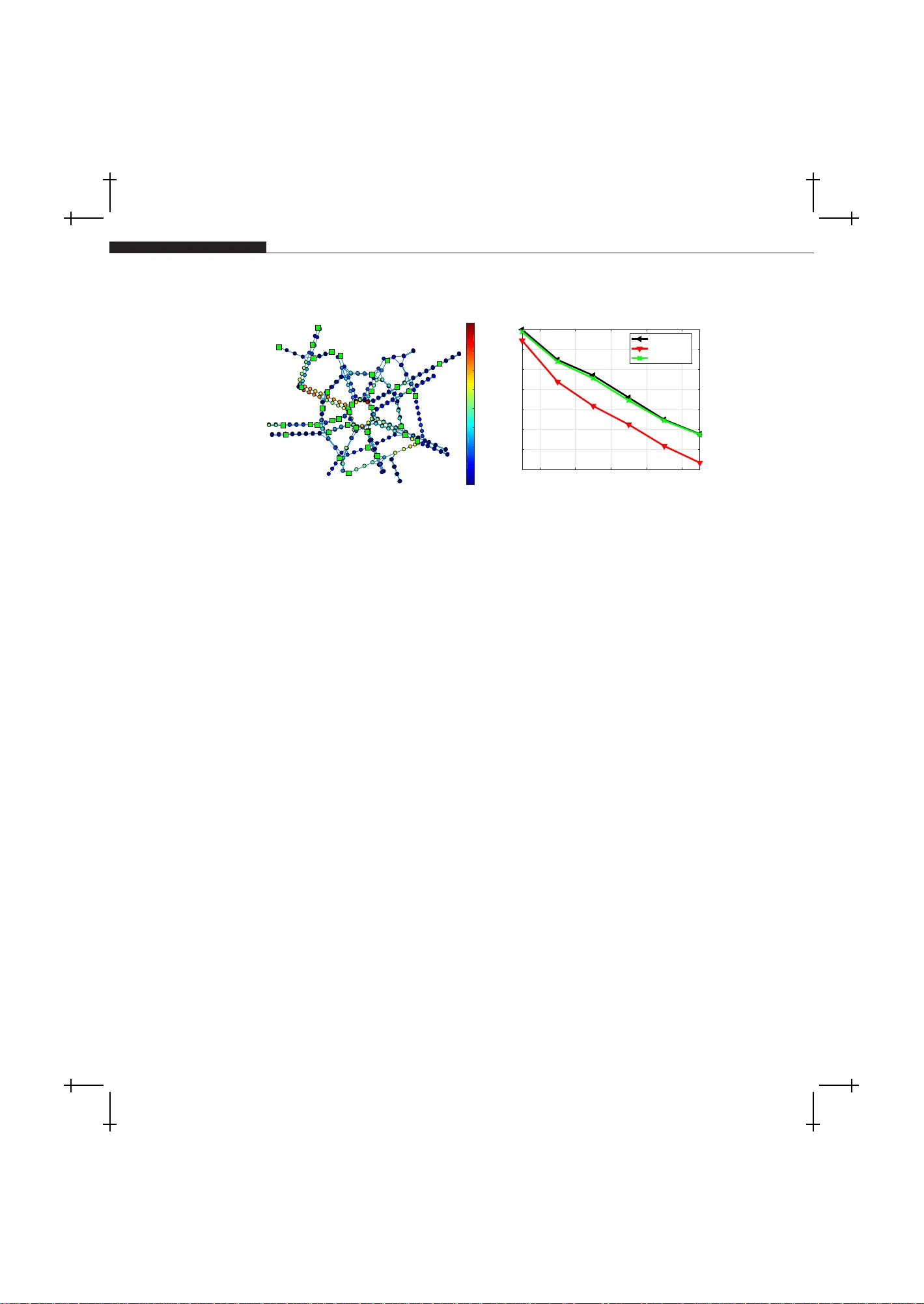
✐ ✐ “Bo ok” — 2 017/12/ 27 — 1:52 — page 1 — #1 ✐ ✐ ✐ ✐ ✐ ✐ Sampling and Recovery of Graph Signals P aolo Di Lo renzo , a, ∗ , Sergio Ba rbarossa, ∗∗ and P aolo Banelli ∗ ∗ University of Perugia, Dep artment of Engine ering, Via G. Dur anti 93, 06125, Perugia, Italy. ∗∗ Sapienza University of R ome, Dep artment of Information Engine ering, Ele ctr onics, and T ele c ommunic ations, via Eudossiana 18, 00184, R ome, Italy. a Corr esp onding: paolo.dilorenzo@unip g.it ABSTRACT The aim of this c hapter is to giv e an o verview o f t h e rece nt adv ances related to sam- pling and recove ry of signals defined o ver graphs. First, w e illustrate the conditions for p erfect recov ery of bandlimited graph signals from samples collected ov er a se- lected set of vertexes. Then, w e describ e some sampling design criteria prop osed in the literature to mitigate the effect of noise and mo del mismatc hing when p erform- ing graph signal reco very . Finally , w e illustrate algorithms and optimal sampling strategies for adaptive recov ery and tracking of dynamic graph signals, where b oth sampling set and signal v alues are allo wed to v ary with time. Numerical sim ulations carried out o ver b oth synthetic and real data illustrate the p oten tial adv antages of graph signal pro cessing metho ds for sampling, interpolation, and trac king of signals observed ov er irregular domains such as, e.g., technologi cal or b iolog ical netw orks. Keyw ords: Graph signal pro cessing, sampling on graphs, interpolation on graph s, adaptation and learning o ver netw orks 1.1 INTRODUCTION In a large num ber of a pplications inv olving senso r , transp ortation, communi- cation, so cial, or biolog ical netw ork s, the obser v ed data can b e mo deled as signals defined ov er g raphs, or graph sig nals for s hort. As a consequence, ov er the la st few years, there was a surg e of in terest in developing nov el ana lysis metho ds for graph signa ls, thus leading to the research field known as gra ph signal pro cessing (GSP), see, e.g., [1, 2]. The g oal of GSP is to ex tend classica l pro cessing to ols to the analy sis of signals defined over an irre gular discrete do- main, re pr esen ted by a gr aph, and one in teresting asp ect is that such metho ds 1 ✐ ✐ “Bo ok” — 2 017/12/ 27 — 1:52 — page 2 — #2 ✐ ✐ ✐ ✐ ✐ ✐ 2 Chapter Title t ypically come to dep end on the graph top olog y , see, e.g., [2, 3, 4, 5, 6 ]. A fundamen tal task in GSP is to infer the v alues of a graph signa l by inter- po lating the samples collected from a known set of vertices. In the GSP liter- ature, this learning task is k nown as interp olation fr om samples , and emerges whenever cost cons tr ain ts limit the n umber of vertices that w e can directly observe. This aris es in several applications such as s emi-super vised learning of categoric al data [7], environment al monitoring [8], and missing v a lue pr edic- tion as in matrix completion pr oblems [9 ]. Int erp olation metho ds on graphs rely on the implicit assumption that no des close to ea c h other ha ve similar v alues, i.e., the graph enco des s imila rit y a mong the v alues observed over the vertices. F or instance, in an item-item gr a ph in a recommendatio n system, a use r would rate tw o similar items with simila r ra ting s [10]. In the s ame wa y , predicting the functions of pr oteins based on a pr otein net work relies on some notion o f clos eness among the no des [11]. In other words, the signa ls of int eres t must be smo oth functions ov er the gra ph. In GSP , the smo othness assumption is typically formalized in terms of (approximate) ba ndlimitedness ov er a graph F ourier basis, and enables rec o very of the signal a fter sampling ov er a selected subset of vertices. A first se mina l con tribution to sampling theo r y in GSP is given by [12], where a sufficient condition for unique rec o very is stated for a given sampling set; the approach was then extended in [1 3, 1 4]. Mos t of the works on g raph sampling theory assume tha t a po rtion o f the gr aph F ourier basis is explic- itly known. F or example, the work in [6 ] pro vides conditions that guarantee unique reco nstruction of signals spanned over a subset of vectors comp osing the gr aph F ourier ba s is, prop osing also a greedy metho d to selec t the sampling set in o rder to minimize the effect of s ample noise in the worst-case. Refere nce [15] exploited a smart partitioning of the gra ph in lo cal-sets, and prop osed it- erative metho ds to reconstruct bandlimited gr aph signal from sa mpled data. The work in [16] creates a conceptual link betw een uncerta in ty principle and sampling of graph s ignals, and pr o pose s several optimality cr iteria (e.g., the mean-squar e error ) to select the sa mpling set in the presence of nois e . An- other v a lid approach is the so-calle d ag g regation sampling [1 7], which inv olves successively shifting a signal using the adja c ency matrix a nd ag gregating the v alues at a given no de. Greedy s ampling stra tegies with prov able p erformance guarantees were prop osed in [1 8] in a Bay esian reco nstruction setting. If the size o f the graph signal is very large as, e.g., in web-scale gra phs [19], complexity b ecomes a crucial issue, such that in many ca ses we cannot ass ume to know or efficiently compute the graph F o urier basis. So me works hav e then prop osed sampling metho ds that do not requir e such previous knowledge. F or instance, the work in [20] pro poses efficient metho ds to sele c t the sampling s et based o n powers of the v a r iation op erator to approximate the bandwidth of the g raph signa l. There a re also a lternative appro ac hes that do no t consider graph s p ectral informatio n and rely only on vertex-domain characteristic, e.g., ✐ ✐ “Bo ok” — 2 017/12/ 27 — 1:52 — page 3 — #3 ✐ ✐ ✐ ✐ ✐ ✐ 1.2 Notati on and Background 3 maximum gr aph cuts [2 1] a nd spanning trees [22]. Fina lly , ther e exist ran- domized sa mpling stra tegies, e.g., [2 3, 24, 2 5]. The work in [23] provides an efficient design o f sampling pr obabilit y distribution ov er the nodes , deriving bo unds on the reconstruction error in the presence of noise and/or approx- imatively bandlimited signals. Reference [24] exploits compressive sa mpling arguments to deriv e random sampling strategies with v ar ia ble densit y , th us also pr opos ing a fast technique to estimate the optimal sampling distribution accurately . Last, the w ork in [2 5] pr o pose s a sampling str ategy tailo r ed for large-s cale da ta ba sed on random walks on g raphs. The sampling strategie s describ ed so far in volve batch methods for sam- pling and r e co very of graph signals . In many applications such a s, e.g., trans- po rtation netw ork s, brain netw o rks, or communication netw o rks, the o bserved graph s ig nals are typically time-v arying. This req uires the developmen t of ef- fective metho ds ca pable to learn and tra c k dynamic gra ph s ig nals fro m a carefully designed, p ossibly time-v arying , sampling set. Some previo us works hav e considered this sp ecific lea rning task, s ee, e.g., [26, 27, 28, 29]. Specif- ically , [26] prop osed an LMS es timation stra tegy enabling a daptiv e learning and tra c king from a limited num ber of s martly sampled obse r v ations. The LMS metho d in [2 6] was then extended to the distributed setting in [27]. The work in [28] prop osed a kernel-based re construction framework to accommo - date time-evolving signals o ver p ossibly time-evolving top ologies, leveraging spatio-temp oral dynamics of the o bserved data. Finally , reference [29] pro- po ses a distributed method for tra c king bandlimited graph signals, ass uming per fect o bs erv ations a nd a fixed sampling stra teg y . In this chapter, we review some o f the rec en t adv ances related to sampling and recov ery of signals defined over gra phs. Due to space limitations, such review will be limited only to some specific contributions. The structure o f the chapter is expla ined in the s e quel. Sec. 1 .2 defines the adopted notation, and reca lls some background on GSP . In Sec. 1.3, we illustra te the co nditions for perfect recov ery of bandlimited graph signa ls from sa mples collected ac- cording to design criter ia propo sed to mitigate the effect of nois e or mo del mismatching. Finally , Sec. 1 .4 illustrates algorithms and optimal sampling strategies for ada ptiv e recovery and tracking of dy namic graph signals , where bo th sa mpling set and signa l v alues are allow ed to v a ry with time. 1.2 NOT A TION AND BA CK GROUND In this par agraph, we fir st introduce the notation tha t we will use throughout the c hapter. Then, we briefly recall some basic notions fr o m GSP that w ill be ins trumen tal for the deriv atio ns and arguments of the following sections. Notation. W e indica te scalars b y normal letters (e.g., a ); vector v ariables ✐ ✐ “Bo ok” — 2 017/12/ 27 — 1:52 — page 4 — #4 ✐ ✐ ✐ ✐ ✐ ✐ 4 Chapter Title with b o ld lowercase letters (e.g., a ) and matrix v aria bles with b old upper c ase letters (e.g., A ). Scalars a i and a ij corres p ond to the i - th entry of a and the ij -th en try of A , re spectively . W e indicate by k a k 2 and k A k 2 the ℓ 2 norm and the s pectral norm of the vector a and matr ix A , resp ectiv ely . If A is rectangular , we denote b y σ i ( A ) the i -th s ing ular v alue of A ; if A is squa re, λ i ( A ) represe nts the i - th eig en v alue of A . The tra ce op erator of matrix A is indicated with T r( A ); diag( a ) is a diago nal matrix having a a s main diagona l; rank( A ) denotes the rank o f matrix A ; det( A ) represents the determinant of A , wher eas pdet ( A ) is the pse udo -determinant of A , i.e., the pr o duct of a ll non-zero eigenv alues of A . The sup e r script H denotes the her mitian op erator, i.e., the conjuga te transp osition of a vector or a matrix , whereas A † denotes the pseudo-inverse of matrix A . E { ·} represents the exp ectation op erator. A set o f ele ments is denoted by a callig raphic letter (e.g., S ), and |S | re pr esen ts the cardinality of set S , i.e., the nu mber of elemen ts of S . The sym b ols ∪ , ∩ , and \ denote union, int ers e ction, and difference among s ets, res pectively . Given a set S , we denote its complemen t set as S c , i.e., V = S ∪ S c and S ∩ S c = ∅ . 1 denotes the vector of all ones, whereas 1 S is the set indicator vector, whose i -th entry is e q ual to one, if i ∈ S , or zer o otherw is e. Bac kground. W e consider a graph G = ( V , E ) consisting o f a set of N no des V = { 1 , 2 , ..., N } , along with a se t of weigh ted edges E = { a ij } i,j ∈V , such that a ij > 0 , if there is a link fro m no de j to no de i , or a ij = 0, otherwise. The adjacency matrix A of a gra ph is the co llection of all the weigh ts a ij , i, j = 1 , . . . , N . The combin ator ial Laplacian matrix is defined as L = diag( 1 T A ) − A . A signal x over a gr a ph G is defined a s a mapping from the vertex set to the s e t of complex num b ers, i.e., x : V → C . The gra ph G is endowed with a graph-shift o pera tor S defined as an N × N ma trix whose entry ( i, j ), denoted with S ij , can be no n-zero only if i = j or the link ( j, i ) ∈ E . The spa rsit y pattern of matrix S captures the loca l structure of G ; c o mmon choices for S are the adjacency matrix [2], the Laplacian [1], and its generalizations [20]. W e assume that S is diagona liz able, i.e., ther e exists an N × N matrix U = [ u 1 , . . . , u N ] and an N × N diagonal ma trix Λ that can b e used to de c ompose S as S = UΛU − 1 . When S is norma l, i.e., when SS H = S H S , matrix U is unitary and U − 1 = U H . Recov ery of a signal from its sampled version is pos sible under the assump- tion that x a dmits a sp arse r epr esentation . The basic idea when addressing the problem of sampling graph signals is to supp ose that S plays a key role in explaining the s ignal o f interest. More sp ecifically , w e assume that x can b e expressed as a linear combination of a subset o f the columns of U , i.e., x = U s (1.1) where s ∈ C N is either exactly or approximately spa rse. In this context, vec- tors { u i } N i =1 are interpreted as the gr aph F ourier basis, and { s i } N i =1 are the ✐ ✐ “Bo ok” — 2 017/12/ 27 — 1:52 — page 5 — #5 ✐ ✐ ✐ ✐ ✐ ✐ 1.2 Notati on and Background 5 corres p onding g raph sig nal frequency co efficien ts, i.e., s = U H x (1.2) takes the role of the Graph F ourie r T ransfor m (GFT) o f signal x . As a n example, in man y cases the gr aph signal exhibits clustering fea tures, i.e., it is a smo oth function over each c luster (e.g., in semi-supe r vised le a rning [7]), but it may v ary ar bitrarily from one clus ter to the other. In such a case, if the columns of U are chosen to r e present clusters, the only nonzer o (or approximately nonzero) entries o f s are the ones ass ocia ted to the clusters. In the ca se of undir e cte d g r aphs, U ma y b e c o mposed fr om the eigen vectors of the Laplacian, which hav e well known clustering prop erties [30]. The lo calization pro perties of graph signals in vertex and frequency do - mains will play an impo rtan t role in the ensuing ar gumen ts. T o intro duce such prop erties, we first define the matrix U F ∈ C N ×|F | , which r epresents the collection of all the columns of U asso ciated with a subset o f frequency indices F ⊆ { 1 , . . . , N } . Then, we introduce the N × N band-limiting op erator B F = U F U H F . (1.3) The ro le of B F is to pro ject a vector x onto the subspace spa nned by the columns of U F . Thus, we say that a vector x is perfectly lo calized ov er the frequency set F (o r F -bandlimited) if B F x = x = U F s F , (1.4) where B F is given in (1.3), and the second equality comes from (1.1) where we have e xploited the s pa rsit y of s , whic h is differen t from zero (and equal to s F ∈ C |F | ) o nly in the frequency supp ort F . Similar ly , giv en a subset of vertices S ⊆ V , we define the N × N v ertex- limiting op erator D S = dia g { 1 S } . (1.5) Thu s, w e s a y that a v ector x is p erfectly loca lized over the subse t S ⊆ V (or S -vertex-limited) if D S x = x , with D S defined a s in (1.5). W e als o denote by B F the set of a ll F -bandlimited signals, and by D S the set of a ll S -vertex- limited sig nals. The oper ators D S and B F are self-a djoin t and idempotent, and repres en t orthogonal pro jector s ont o the sets D S and B F , res pectively . Different ly fro m contin uo us-time signa ls, a graph signal can be per fectly lo cal- ized in b oth vertex and frequency domains. This pr oper t y is formally stated in the following theorem [16, Th. 2.1]. Theorem 1. Ther e is a gr aph signal x p erfe ctly lo c alize d over b oth vertex set S and fr e quency set F (i. e. x ∈ B F ∩ D S ) if and only if the op er ator B F D S B F has an eigenvalue e qual to one; in su ch a c ase, x is the eigenve ctor of B F D S B F asso ciate d to the u nit eigenvalue. ✐ ✐ “Bo ok” — 2 017/12/ 27 — 1:52 — page 6 — #6 ✐ ✐ ✐ ✐ ✐ ✐ 6 Chapter Title Perfect lo calizatio n onto the sets S and F can b e equiv alently e xpressed in terms of the o pera tor D S U F [16], i.e., it holds if and o nly if k D S U F k 2 = k B F D S B F k 2 = 1 . (1.6) In the following section, we will illustrate the theory b ehind sampling a nd recov ery of sig na ls defined ov er gr a phs. 1.3 SAMPLING AND RECO VERY Let us consider the observ ation of an F -bandlimited gra ph signal ov er the sampling set S . The observ ation mo del can b e cast as : y S = P T S x = P T S U F s F , (1.7) where y S ∈ C |S | is the o bserv ation vector ov er the vertex set S , a nd P S ∈ R N ×|S | is a sa mpling matrix whose columns are indicator functions for no des in S , and such that the orthog onal pro jector ov er D S is given by D S = P S P T S [cf. (1.5)]. The pro blem of r ecov er ing a bandlimited graph signal from its samples is then equiv alent to the problem of prop erly selecting the sampling set S , and then r eco ver x fro m y S by in verting the system of equatio ns in (1.7). This appro ac h is kno wn as sele ction sampling and was address ed, for example, in [12], [13], [6 ], a nd [16]. In the s equel, we will first consider the conditio ns for p erfect recovery of bandlimited g raph signa ls. Then, we will illustrate the effect of noise and mo del mismatching on the reconstruc tio n p erformance. Also , since the iden- tification of the sa mpling set S pla ys a key role in the c onditions for signa l recov ery a nd in the reconstruction perfor mance, w e will illus trate o ptimiza- tion stra tegies to design the sampling set. Finally , we will illustrates re sults of num erica l simulations carried out ov er synthetic a nd realistic data. 1.3.1 SAMPLING AND PERFECT RECOVERY OF BANDLIMITED GRAPH S IGNALS W e will no w address the fundamental problem of assess ing the co nditions and the means fo r p erfect recov ery of x fr om y S . T o this aim, we introduce the o pera tor D S c = I − D S , whic h pr o jects on to the complemen t v ertex set S c = V \ S . Starting from (1.7), the necessary and sufficient conditions for per fect r e co very are stated in the following Theo rem [16, Th. 4.1]. Theorem 2 . Any F -b and limite d gr aph signal x c an b e p erfe ctly r e c over e d fr om its samples c ol le cte d over t he vertex s et S if and only if k D S c U F k 2 < 1 , (1.8) ✐ ✐ “Bo ok” — 2 017/12/ 27 — 1:52 — page 7 — #7 ✐ ✐ ✐ ✐ ✐ ✐ 1.3 Sampl ing and Recovery 7 i.e., if ther e ar e no F - b and limite d signals that ar e p erfe ctly lo c alize d on S c . Pr o of. F rom (1.7), a sufficie nt condition for signal r e c o very is the existence of the pseudo-inv erse matrix Q = ( P T S U F ) † = ( U H F D S U F ) − 1 U H F P S . Since U H F D S U F = I − U H F D S c U F , we obtain that Q exists if k U H F D S c U F k 2 = k D S c U F k 2 < 1, i.e., if (1.8) holds true. Co n versely , if k D S c U F k 2 = 1 , there exist bandlimited s ignals that are per fectly lo calized ov er S c [cf. (1.6)]. Thus, if we s ample one o f s uc h signals ov er S , it w o uld b e imp ossible to recover x from those samples. This prov es that condition (1.8) is also necessar y . Theorem 2 a nd its pr oof also suggest the reconstructio n formu la: b x = U F ( P T S U F ) † y S = U F ( U H F D S U F ) − 1 U H F P S y S , (1.9) which g uarantees reconstruction of the bandlimited graph signa l x if co ndition (1.8) holds true, and ha s computational complexity equal to O ( N |F | 2 ). The ab o ve reconstruction formula is also kno wn as co nsisten t re c onstruction [31] since it keeps the observed samples unchanged. Let us consider no w the implications of condition (1.8) o f Theorem 2 on the sampling strategy . T o fulfill (1.8), we nee d to gua rant ee that there exist no signals that ar e p erfectly lo calized ov er the vertex set S c and the freq ue nc y set F . Since, in genera l, w e hav e y S = P T S U F s F + P T S c U F s F , (1.10) we need to g uarantee that P S U F s F 6 = 0 ¯ for any non-trivial vector s F , which requires P T S U F to b e full column rank, i.e., rank( P T S U F ) = rank( U F ) = |F | . (1.11) Of course, a necessary condition to sa tisfy (1.1 1 ) is that |S | ≥ |F | . (1.12) How ever, condition (1.12) is not sufficient, b ecause P T S U F may lo ose ra nk, depe nding on g raph topolo gy and sa mples’ lo cation. As a particular ca se, if the gra ph is no t co nnected, the v ertices can b e lab eled so that the Laplacia n (adjacency) matrix ca n b e written as a blo ck diago nal ma trix, with a num b er of blo c ks equal to the nu mber of connected co mponents. Corresp ondingly , each eig en vector of L can be ex pressed as a vector having all zer o ele ments, except for the ent ries co rresp onding to the connected comp onen t. This implies that, if there are no samples ov er the vertices corres ponding to the non-null en- tries o f the eigenv ec tors with index included in F , P T S U F lo oses rank. More generally , even if the graph is connected, ther e may easily o ccur s itua tions where matrix P T S U F is not rank-defic ie nt, but it is ill-conditioned, dep ending on graph topo logy a nd samples’ lo cation. This case is particula rly dangero us when the tr ue signal is only approximately bandlimited (which is the ca s e for ✐ ✐ “Bo ok” — 2 017/12/ 27 — 1:52 — page 8 — #8 ✐ ✐ ✐ ✐ ✐ ✐ 8 Chapter Title most signals in pr a ctice) or when the samples ar e nois y . In such cases, not all sampling sets of given size are equally go o d, and it beco mes fundamen- tal to understand which is the b est sampling set that achiev es the smallest reconstructio n err o r. Th us, in the sequel, we will first illustrate the effect o f noise and mo del mismatching o n graph sig na l reconstruction, and then we will describ e sampling strategies satisfying several o ptimization c riteria. 1.3.2 THE EFFECT OF NOISE AND MODEL MISMA TCHING Let us co nsider first the r econstruction of bandlimited sig na ls from no is y s am- ples, where the observ a tion mo del is given by: y S = P T S ( x + v ) = P T S U F s F + P T S v , (1.13) where v is a zero- mea n noise vector with cov ar ia nce matrix R v = E { vv H } . T o des ig n an interpolato r in the presence o f noise, we consider the b est linear un biased estimator (BLUE), which is given by [32]: b x = U F  U H F P S  P T S R v P S  − 1 P T S U F  − 1 U H F P S  P T S R v P S  − 1 y S . (1.14) The estimator in (1.14) minimizes the le a st square erro r and, if noise is Gaus - sian in (1.27), it coincides with the minimum v ariance unbiased estimator , which attains the Cr am ´ er-Rao lower bo und. It is immediate to s ee that (1.1 4) is an unbiased estimato r, i.e., E { b x } = x . F urthermo re, the mean square error (MSE) is given by [32]: MSE = E k b x − x k 2 = T r   U H F P S  P T S R v P S  − 1 P T S U F  − 1  . (1.15) As a par ticular case, if nois e is spatially uncorr elated, i.e., R v = diag { r 2 1 , . . . , r 2 N } , and letting u H F ,i be the i -th row of matrix U F , we obtain: MSE = T r n  U H F D S R − 1 v U F  − 1 o = T r    X i ∈S u F ,i u H F ,i /r 2 i ! − 1    . (1.16) This illustrates how, in the prese nce of uncor related noise, the design o f the sampling set should minimize the trace of the in verse of matrix U H F D S R v U F . So far we assumed that the true sig nal x is p erfectly ba ndlimited, i.e., x ∈ B F . How e ver, in most applications, the signals are only approximately bandlimited. In such a case, the r e c o very fo rm ula in (1.9) applied to such signals le a ds to a reconstruction error, which is analyzed ne x t. In gener al, a n approximately bandlimited graph signal can b e ex pressed as x = x F + ∆ x , (1.17) where x F = B F x is the bandlimited comp onent , whereas ∆ x = B F c x rep- ✐ ✐ “Bo ok” — 2 017/12/ 27 — 1:52 — page 9 — #9 ✐ ✐ ✐ ✐ ✐ ✐ 1.3 Sampl ing and Recovery 9 resents the mo del mismatch. S ampling the signal over the v ertex set S and using (1.9) as a recovery for m ula, then an upper b ound (i.e., a w ors t-case) on the reconstruction err o r is given b y [31]: k b x − x k ≤ k ∆ x k cos( θ max ) , (1.18) where θ max represents the maximum angle b etw een the subspaces B F and D S , which is defined as: cos( θ max ) = inf k z k =1 k D S z k 2 sub ject to B F z = z . (1.19) In pa r ticular, fr om (1.19), it is easy to see that cos( θ max ) > 0 if condition (1.8) holds true. Intuitiv ely , the b ound in (1.18) says that, fo r the worst-case error to b e minim um, the sampling and reco nstruction subspac es should be as alig ned as p ossible. Therefore, for appr o ximatively bandlimited sig nals, an optimal sampling set s hould b e selected in or der to maximize the smallest maximum a ng le b etw e e n the subspac e s B F and D S . Interestingly , from (1.19) and (1.3), it appea rs clea r that cos( θ max ) = σ min ( D S U F ) (1.20) Thu s, in the presence of mo del misma tc hing, the design of the sampling set should maximize the minimum sing ular v alue o f matrix D S U F or, eq uiv a - lent ly , the minimum eigenv alue of matrix U H F D S U F . In the next section, we will illustrate the strategie s used to optimize the selection of the sampling set. 1.3.3 SAMPLING STRA TEGIES As pr eviously mentioned, when sampling graph signals, b esides choosing the right num b er of samples, whenev er p o ssible it is also fundamental to hav e a strategy indicating wher e to sample, as the samples’ lo cation plays a key role in the p erformance o f re construction a lgorithms. In principle, in the ideal case (1.7), any sampling set S that satisfies condition (1 .8) enables unique reconstructio n through the interpo la tion formula in (1.9). How ever, in the presence of no ise or mo del mismatc hing, from (1.16) a nd (1.18)-(1.2 0), it is clear that the quality of recons truction is strongly affected b y a careful desig n of the sampling s e t S . Different costs ca n then be defined to measure the reconstructio n error and are based on optimal design of exp erimen ts [33]. F or instance, if we seek for the optimal sampling set S opt of size M , a s the set that minimizes the mean squared error in (1.16), we hav e: S A − opt = arg min |S | = M T r n  U H F D S R − 1 v U F  − 1 o . (1.21) ✐ ✐ “Bo ok” — 2 017/12/ 27 — 1 :52 — page 10 — #10 ✐ ✐ ✐ ✐ ✐ ✐ 10 Chapter Title Algorithm 1 : Greedy selection of graph samples Input D ata : U F , M ; Output D ata : S , the sampling set. F u n ction : initialize S ≡ ∅ while |S | < M s = arg max j f ( S ∪ { j } ); S ← S ∪ { s } ; end This is analogous to the so - called A-optimal design [33], and is equiv alent to the one pro posed in [16]. Similarly , if we a im to design the optimal sampling set of size M to minimize the worst-case reconstruc tio n erro r in the presence of mo del misma tc hing [cf. (1.1 8)-(1.20)], we hav e: S E − opt = arg max |S | = M σ min ( D S U F ) , (1.22) which is e q uiv a len t to the so-ca lled E-optimal design [33]. The a bov e criterion is equiv alent to the one prop osed in [6 ] and, in general, it is use ful to find a stable sampling set that satisfies condition (1.8). T o s elect the o ptimal sampling set, w e should solve one of the problems in (1.21) o r (1.22), which ent ail the sele ction of an M -element subset of V that optimizes the adopted design cr iterion. This is a finite co m binatorial optimizatio n problem (whic h is known to b e NP- hard [34]), who se s olution in general requires a n exhaustive search over all the p ossible combinations. Since the num b er o f p ossible subsets grows facto rially a s |V | increa ses, a br ute force approach quickly beco mes infeasible also for graph signals o f mo dera te dimensions. T o cop e with this issue, in the sequel, we will intro duce lower complexity metho ds based o n: i) greedy approa c hes, and ii) conv ex rela xations. 1.3.3.1 Greedy Sampling In this section, we will c o nsider a numerically efficient , alb eit sub-optimal, greedy algor ithm to tackle the problem of selecting the s a mpling set. The greedy approa c h is describ ed in Algorithm 1. The s imple idea underly ing such metho d is to iter ativ ely add to the sampling s et those vertices of the g raph that lead to the large s t increment of an adopted p erformance metric, i.e., a sp ecific set function f ( S ) : 2 V → R . W e will set f ( S ) = − T r  ( U H F D S R − 1 v U F ) − 1  if we use an A-optimality design as in (1.21), o r f ( S ) = σ min ( D S U F ) if w e con- sider an E-optimality design as in (1.22). In fact, s ince Algor ithm 1 starts from the empty set, when |S | < |F | , matrix U H F D S R − 1 v U F is inevitably r ank defi- cient, and its inv erse do es not exist. In this case, cons idering an A-optimality criterion, we can use f ( S ) = − T r  ( U H F D S R − 1 v U F ) †  , which b ecomes equiv- ✐ ✐ “Bo ok” — 2 017/12/ 27 — 1 :52 — page 11 — #11 ✐ ✐ ✐ ✐ ✐ ✐ 1.3 Sampl ing and Recovery 11 alent to (1.21) when condition (1.8) is s atisfied. In general, the p erfor mance of the g reedy strateg y will b e sub-optimal with resp ect to an exhaustive search pro cedure. Nev ertheless , if the set func- tion f ( S ) satisfies some str uctural pro perties, the greedy Algor ithm 1 can b e prov ed to b e close to optimality . In particular, submo dula rit y plays a similar role in co m binatorial optimiza tion to conv exity in contin uous optimization and shares other features of concav e functions [35]. Definition 1: A set function f : 2 V → R is submo dular if and only if the derived set functions f a : 2 V \{ a } → R f a ( S ) = f ( S ∪ { a } ) − f ( S ) (1.23) are monotone decreasing , i.e., if for all subsets a, A , B ⊆ V it holds that if A ⊆ B ⇒ f a ( A ) ≥ f a ( B ) . Int uitively , submo dularity is a diminishing returns pr oper t y where adding an element to a s maller set giv es a la rger gain tha n adding one to a larg er s et. The maximiza tion of mono tone increasing submo dular functions is still NP - hard, but the greedy heuristic can be used to obtain a solution that is prov ably close to optimality , with a solution having ob jective v alue within 1 − 1 /e of the optimal combinatorial solution [36]. Unfortunately , b oth set functions in (1.2 1) and (1.2 2) are not submo dular functions 1 [37]. Thus, even if the desig n criter ia in (1.21) a nd (1 .22) are useful to minimize the effect of noise [cf. (1.15)] and mo del mismatching [cf. (1.1 8)- (1.20)], resp ectively , we do not have theo retical p erformance guara n tees when applying Algorithm 1 to so lv e s uc h problems. Nevertheless, in the literatur e of ex perimental design, a further design criterio n is often considered as a surrog ate for (1.21) [or (1.22)], which wr ites as: S D − opt = a rg max |S | = M log det  U H F D S R − 1 v U F  = a rg max |S | = M log det X i ∈S u F ,i u H F ,i /r 2 i ! . (1.24) This is analogo us to the so-called D-optimal design [33], and is eq uiv alent to one of the metho ds pro p osed in [16] for gr aph signals sampling. This design strategy aims at maximizing the volume o f the parallelepip ed built with the selected rows { u H F ,i } i ∈S of matrix U F (w eighted by the in verse of the noise v ariances { r 2 i } i ∈S ), and the rationale is to desig n a well s uited basis for the graph signa l tha t w e wan t to e s timate. Interestingly , the set function 1 In terestingly , in a Bay esian recov ery setting [18] , the negativ e of the MSE function was prov ed to b e appro ximatively submo dular. ✐ ✐ “Bo ok” — 2 017/12/ 27 — 1 :52 — page 12 — #12 ✐ ✐ ✐ ✐ ✐ ✐ 12 Chapter Title f ( S ) = log det( U H F D S R − 1 v U F ) is a monotone increa sing s ubmodular function [38]. Thus, in this case, the greedy appro ac h in Alg orithm 1 can b e used to solve (1.24) with prov able p erformance guarantees. In the implementation o f Algorithm 1, when |S | < |F | and matrix U H F D S R − 1 v U F is rank-deficient, we can use f ( S ) = log pdet( U H F D S R − 1 v U F ), which is equiv alent to (1.24) when sampling condition (1.8) on p erfect recovery is s atisfied. 1.3.3.2 Convex Relaxation Another p ossible alg orithmic s olution to pro ble ms lik e (1.21), (1.22), (1.24), is to resor t to conv ex r elaxation techniques, see, e.g., [39, 40, 41]. T o this a im, let us introduce the indicator vector d = { d i } N i =1 , such that the i-th entry is binary and given by d i = 1 if no de i b elongs to the sampling set S , and d i = 0 otherwise. Using the indicato r vector d , w e can build a general s a mpling design problem that c a n b e cast as: min d f ( d ) s.t. 1 T d = M , d ∈ { 0 , 1 } N , (1.25) where f ( d ) = T r  ( U H F diag( d ) R − 1 v U F ) − 1  for the A-optimal design [cf. (1.21)], f ( d ) = − σ min (diag( d ) U F ) for the E-optimal design [cf. ( 1.2 2)], and f ( d ) = − log det( U H F diag( d ) R − 1 v U F ) for the D-o ptima l design [cf. (1.2 4)]. Problem (1.25) has still combinatorial co mplexit y , due to the in teger nature of the optimization v ariable d . Nevertheless, w e can simple r elax the indica tor v aria ble d to b e a real vector b elonging to the hypercub e [0 , 1] N , thus lea ding to the following formulation: min d ∈ [0 , 1] N f ( d ) s.t. 1 T d = M . (1.26) It is now e a sy to c heck that pr o blem (1.26) is conv ex for all ob jective func- tions f ( d ) defined by the desig n criteria in (1.21), (1 .2 2), (1 .24), and its global solution can be found using efficient n umerical metho ds [4 2]. Of co urse, since (1.26) is a relax ed version of (1.2 5), its real so lution d ∗ might need a further selection/thresho lding step in order to generate a v alid integer vector, as re- quired by (1.25). F or instance, a p ossible s olution is to select the M sampling no des a s the ones asso ciated with the M largest entries of d ∗ . Finally , one can also formulate the sampling desig n problem in the opp osite w ay with resp ect to (1.2 5). In pa rticular, we might be in terested in searching for the optimal indicator vector d tha t minimizes the num b er of co lle cted samples , i.e., the ℓ 0 norm of the vector d , under a p erformance require ment o n the function f ( d ), e.g, the MSE in (1.16). This category of design problems takes the name of ✐ ✐ “Bo ok” — 2 017/12/ 27 — 1 :52 — page 13 — #13 ✐ ✐ ✐ ✐ ✐ ✐ 1.3 Sampl ing and Recovery 13 (a) Graph top ology and sampling set 20 40 60 80 100 Number of samples -8 -7 -6 -5 -4 -3 -2 -1 MSE (dB) D-optimality E-optimality Random A-optimality (b) MSE ve rsus num b er of samples Figure 1.1 Sampling and recovery over the IE EE 11 8 Bus graph sparse sensing [40, 41] and, using similar re laxation arg uments as b efore, suc h criteria lead to conv ex optimizatio n problems. In the next section, we will illustrate some n umerical res ults a imed a t assessing the per formance of the descr ib ed sampling and recov ery stra tegies. 1.3.4 NUMERICAL RESUL TS In the sequel, we cons ider the application of the described sampling and recov ery metho ds to tw o rea l graphs: a power netw or k, and a r oad netw o rk. Sampling o v er p ow er grids. The first example inv o lv es the IEEE 118 Bus T est Case, i.e., a p ortion of the American Electric Po wer Sys tem (in the Mid-w estern US) as o f Decem b er 196 2. The graph is comp osed of 1 18 no des (i.e., bus e s ), its top ology (i.e., tra nsmission lines connecting bus es) is depicted in Fig. 1 .1(a) [4 3], and the co lor of each no de enco des the entries of the eigen vector of the Laplacian matrix asso ciated to the second smallest eigenv a lue (these entries highlight the presence of three distinct cluster s in the net work). As illustrated in [44], the dyna mics of the power generators give ris e to smo oth g raph signals, so that the bandlimited assumption is jus- tified, although in approximate se ns e. In our ex ample, we randomly gener ate a lowpass signal with |F | = 1 2 a nd w e ta k e a num b er o f samples equal to |S | = 12. The green squa res corresp ond to the samples selected using the greedy Alg o rithm 1 a nd the A-optimality design in (1.21). It is interesting to see how the metho d distributes sa mples ov er the clus ters, and puts the s a m- ples, within each clus ter, quite fa r apart from each other. Finally , we compar e the r econstruction p erforma nce obtained b y the cons idered greedy sampling strategies [cf. (1.21), (1.22), and (1.24)] and by random sampling. T o this aim we consider gra ph s ignal rec o very , in the pres ence of an uncorr elated, zero ✐ ✐ “Bo ok” — 2 017/12/ 27 — 1 :52 — page 14 — #14 ✐ ✐ ✐ ✐ ✐ ✐ 14 Chapter Title 0 2 4 6 8 10 12 14 16 (a) Graph topology and sampling set 10 20 30 40 50 Bandwidth -16 -15 -14 -13 -12 -11 -10 -9 NMSE (dB) D-optimality E-optimality A-optimality (b) NMSE ve rsus bandwidth Figure 1.2 Sampling and recovery of vehicular flows over road net wo rks mean Gaussia n ra ndom noise with unit v a riance, a nd considering |F | = 20 . Thu s, Fig. 1.1(b) repor ts the MSE in (1.1 6) v ersus the num b er of samples collected ov er the gr aph. As expected, the MSE decrease s as the n umber of samples increa ses. W e can also notice how r andom sa mpling perfo rms quite po or ly , wherea s the A-optimal design (and the D-optimal desig n) outp erforms all other strategies . T raffic flo w prediction o v er road netw orks. The seco nd exa mple consid- ers sa mpling of a p ortion of the roa d netw ork in the neig h b orho od of Mazzini square, which is in the city of Rome, Italy . W e hav e placed landmark s (no des of the graph) over the streets in a r e gular fashion, and c onnected adjacent landmarks on the same la ne and at the junctions, th us obtaining the gra ph top ology depicted in Fig. 1.2(a). The sig nal lying o n the vertices of the graph re present s the flow (num b er of vehicles per unit of time) of ca rs passing through the landma rks during a per io d of 30 seco nds, a nd was obtained using a r ealistic simulator of urban mobility , namely , SUMO [45]. The similarity of v alues of the signal ov er adjacent no des makes the signal to b e s mo oth, but only approximatively bandlimited. In this s ense, there is a mismathcing b e- t ween the observed sig nal and the bandlimited mo del us ed for pr ocess ing. The goal is to infer the traffic situation ov er all the road netw ork from a small num- ber of collected samples. Thus, we cons ider a bandwidth equal to |F | = 30, and we take a n umber of sa mples equal to |S | = 40. The green s quares in Fig. 1.2(a) corres pond to the samples selected using the convex relaxation in (1.26) and the E-optimality design in (1 .22). It is in teresting to see how the metho d distributes a lmost unifor mly the samples ov er the streets and the junctions. Finally , w e compare the reconstruction p erforma nce obtained by the sampling stra tegies bas e d on conv ex relaxation [cf. (1.21), (1.22), and (1.24)] in the presence of mo del mismatching. T o this aim, Fig . 1.2(b) re- ✐ ✐ “Bo ok” — 2 017/12/ 27 — 1 :52 — page 15 — #15 ✐ ✐ ✐ ✐ ✐ ✐ 1.3 Sampl ing and Recovery 15 po rts the normalized MSE (NMSE), i.e., NMSE = k b x − x k 2 / k x k 2 , versus the graph signal ba ndwidth, and selecting |S | = |F | . F rom Fig. 1.1(b), as ex- pec ted, the NMSE decreases if we use a large r bandwidth. F ur ther more, in this case , the E-optimal design o utperforms all o ther strategies, a s expected from (1.18)-(1.20). 1.3.5 ℓ 1 -NORM RECONSTRUCTION OF GRAPH SIGNALS Let us consider now a differe n t obser v ation mo del, where a bandlimited graph signal x ∈ B F is observed everywhere, but a subset of node s S is strongly corrupted by noise, i.e., y = x + D S v , (1.27) where the noise is arbitrary but b ounded, i.e., k v k 1 < ∞ . This model is rele - v ant, for e x ample, in s e nsor netw ork s , where a subset of sensors can b e dam- aged or highly int erfer ed. The problem in this case is whether it is possible to recover the g raph signal x exa ctly , i.e., irresp ective of nois e . Even though this is not a sampling problem, the solution is still related to sampling theory . Clearly , if the s ignal x is bandlimited a nd if the indexes o f the no isy obser - v ations are kno wn, the answer is simple: x ∈ B F can b e p erfectly r ecov er ed from the noisy-free observ atio ns, i.e., by co mpletely discar ding the noisy ob- serv atio ns, if the sampling theorem condition (1.8) ho lds true. But of course, the challenging situatio n o ccurs when the lo cation of the noisy observ ations is not known. In s uc h a case, we may r esort to a n ℓ 1 -norm minimization, by formulating the problem as follows [16]: b x = arg min x ∈B k y − x k 1 . (1.28) W e pr o vide next some theore tical b ounds on the cardinalit y of S and F en- abling per fect recovery of the ba ndlimited g raph signal us ing (1.2 8). T o this purp ose, we recall the following lemma from [1 6]. Lemma 1. L et us define µ := max j ∈F i ∈V | u j ( i ) | , wher e u j ( i ) is the i -th entry of the j -t h ve ctor of t he gr aph F ourier b asis. If for some u nknown S , we have |S | < 1 2 µ 2 |F | , (1.29) then the ℓ 1 -norm r e c onstruction metho d (1.28) r e c overs x ∈ B p erfe ctly, i.e. b x = x , for any arbitr ary noise v pr esent on at most |S | vertic es. An example o f ℓ 1 reconstructio n based on (1.28) is useful to grasp so me int eres ting featur es. W e consider the IEEE 118 bus g raph in Fig . 1.1(a). The signal is as sumed to b e bandlimited, with a sp ectral conten t limited to the first |F | eigenv ectors o f the Laplacian matrix. In Fig. 1.3, we rep ort the b eha vior of ✐ ✐ “Bo ok” — 2 017/12/ 27 — 1 :52 — page 16 — #16 ✐ ✐ ✐ ✐ ✐ ✐ 16 Chapter Title 20 40 60 80 100 Number of noisy samples -100 -90 -80 -70 -60 -50 -40 -30 -20 NMSE (dB) Figure 1.3 ℓ 1 -norm reconstruction: NMSE versus numb er of noisy samples. the NMSE asso ciated to the ℓ 1 -norm estimate in (1.28) , versus the num b er of noisy samples, considering different v alues of bandwidth |F | . As we can notice from Fig. 1.3, for any v a lue of |F | , there exists a threshold v a lue such that, if the num ber of nois y samples is low er than the thresho ld, the re c onstruction o f the signa l is error free. As exp ected, a smaller sig nal bandwidth allows per fect reconstructio n with a la rger num b er of noisy samples. 1.4 AD A PTIVE SAMPLING AND RECO VE RY In this section, w e consider pr o cess ing methods capable to learn and track dynamic graph signals from a ca refully designe d, p ossibly time-v arying , sam- pling set. T o this aim, let us a ssume tha t, at each time n , no isy samples of the signal ar e taken ov er a (randomly) time-v arying subset of vertices, according to the following model: y [ n ] = D S [ n ] ( x + v [ n ]) = D S [ n ] U F s F + D S [ n ] v [ n ] (1.30) where D S [ n ] = diag { d i [ n ] } N i =1 ∈ R N × N [cf. (1.5)], with d i [ n ] denoting a r a n- dom sampling binary co efficient , which is equal to 1 if i ∈ S [ n ], and 0 oth- erwise (i.e., S [ n ] represents the instantane ous , random sampling set at time n ); and v [ n ] ∈ C N is zer o-mean, spatially and temp orally indep endent obse r - v ation noise, with c ov ar ia nce matrix R v = dia g { r 2 1 , . . . , r 2 N } . The estimatio n task co nsists in recov ering the vector x (or, equiv a len tly , its GFT s F ) fr o m the noisy , s treaming, and partial observ ations y [ n ] in (1.30). F ollowing an LMS appr oach [46], from (1.3 0), the optimal e stimate for s F can b e found as the vector that solves the following optimization problem: min s E k D S [ n ] ( y [ n ] − U F s ) k 2 (1.31) ✐ ✐ “Bo ok” — 2 017/12/ 27 — 1 :52 — page 17 — #17 ✐ ✐ ✐ ✐ ✐ ✐ 1.4 Adapt ive Sampling and Recovery 17 Algorithm 2 : LMS on Graphs Start with random b x [0]. Giv en a step-size µ > 0, for n ≥ 0, rep eat: b x [ n + 1] = b x [ n ] + µ B F D S [ n ] ( y [ n ] − b x [ n ]) . where in (1.3 1) w e hav e exploited the fact that D S [ n ] is an idemp oten t matrix for any fixed n [cf. (1.5)]. An LMS-t yp e solution optimizes (1.31) by means of a stochastic steep est-descent pro cedure, relying only on instan taneous in- formation. Thus, letting b x [ n ] be the current estimates of vector x , the LMS algorithm for graph s ignals evolves as illus trated in Algor ithm 2 [26]. In the se q uel, w e illustr a te how the desig n of the sampling strategy affects the reco nstruction ca pabilit y of Algor ithm 2 . T o this aim, let us denote the exp e cte d sampling set b y S = { i = 1 , . . . , N | p i > 0 } , i.e., the set of no des of the g raph that ar e sampled with a probability p i = E { d i [ n ] } strictly greater than zer o. Also , let S c be the co mplemen t set of S . Then, the following r esults illustrates the conditions for adaptive recov ery of gr aph signals [26, 47]. Theorem 3. Any F -b and limite d gr aph signal c an b e re c onstructe d via the adaptive Algorithm 2 if and only if   D S c U F   2 < 1 , (1.32) i.e., if ther e ar e no F - b and limite d signals that ar e p erfe ctly lo c alize d on S c . Different ly from batch sampling and recov ery of graph signals, see, e.g., [12, 13, 6, 16, 17], condition (1.3 2) dep ends on the ex p e cte d sampling s et. In particular , it implies that ther e are no F -bandlimited signals that are p erfectly lo c a lized ov er the set S c . As a co nsequence, the a daptiv e Algo rithm 2 with proba bilistic sampling do es not need to collect a ll the data necessary to reconstruct one- shot the gr a ph signal at each itera tion, but ca n learn acquiring the needed information ov er time. The only impor tan t thing required by c o ndition (1.32) is that a sufficient ly lar ge num b er of no de s is sa mpled in exp e ctation . W e now illustra te the mean- square p erformance o f Algorithm 2. The main results are summarized in the following Theorem [47]. Theorem 4. Assume sp atial and temp or al indep endenc e of the r andom vari- ables ext r acte d by the sampling pr o c ess { d i [ n ] } i,n . Then, for any initial c ondi- tion, Algorithm 2 is me an-squar e err or stable if t he sampling pr ob ability ve ct or p and the step-size µ satisfy (1.32) and 0 < µ < 2 λ min  U H F diag( p ) U F  λ 2 max  U H F diag( p ) U F  . ✐ ✐ “Bo ok” — 2 017/12/ 27 — 1 :52 — page 18 — #18 ✐ ✐ ✐ ✐ ✐ ✐ 18 Chapter Title F u r t hermor e, un der a s mal l step-size assumt pio n, the MSE writes as: MSE = lim n →∞ E k b x [ n ] − x [ n ] k 2 = µ 2 T r h  U H F diag( p ) U F  − 1 U H F diag( p ) R v U F i (1.33) and the c onver genc e r ate α is wel l appr oximate d by α = 1 − 2 µλ min  U H F diag( p ) U F  . (1.34) The results of Theor em 5 are instrumental to devise optimal pro babilistic sampling strategies for Algorithm 2, whic h ar e describ ed in the sequel. 1.4.1 PROBABILI STIC SAMPLING STRA TEGIES W e c o nsider a sampling des ig n that seeks for the pro ba bilit y vector p that minimizes the to tal sampling rate ov er the graph, i.e., 1 T p , while guaranteeing a target p erformance in terms of MSE in (1.33) and of con vergence r ate in (1.34) [47]. Then, the optimization pr oblem c an b e cast a s: min p 1 T p s.t. λ min  U H F diag( p ) U F  ≥ 1 − ¯ α 2 µ , T r h  U H F diag( p ) U F  − 1 U H F diag( p ) R v U F i ≤ 2 γ µ , 0 ≤ p ≤ p max . (1.35) The first constraint imp oses that the co n vergence rate of the alg orithm is larger than a desir ed v alue, i.e., α in (1.34) is smaller than a targ et v alue, say , e.g., ¯ α ∈ (0 , 1). F ur ther more, as illustra ted in [47], the first cons train t on the conv ergence r ate also guarantees adaptive signal rec onstruction, i.e., condition (1.32) holds true. The second co nstraint gua r an tees a ta r get mean- square p erformance, i.e., the MSE in (1.33) must b e less than o r e q ual to a prescrib ed v a lue, say , e.g ., γ > 0. Fina lly , the last constraint limits the probability vector to lie in the box p i ∈ [0 , p max i ], for a ll i , with 0 ≤ p max i ≤ 1 denoting an upp er b ound o n the sampling pro babilit y at each no de that might depe nd on exter nal factors such as, e.g., limited e ne r gy , pro cessing , and/or communication resour ces, no de or communication failure s, etc. Unfortunately , pro ble m (1.35) is no n- con vex, due to the presence of the non-conv ex cons train t o n the MSE. T o handle the non-convexit y o f (1.35), we exploit an upper bound o f the MSE function in (1.33), given b y: MSE( p ) ≤ MSE( p ) , µ 2 T r  U H F diag( p ) R v U F  λ min  U H F diag( p ) U F  , for all p ∈ R N . (1.36) ✐ ✐ “Bo ok” — 2 017/12/ 27 — 1 :52 — page 19 — #19 ✐ ✐ ✐ ✐ ✐ ✐ 1.4 Adapt ive Sampling and Recovery 19 Of course, replacing the MSE function with the b ound (1.36), the s econd constraint in (1.35) is alwa ys satisfied. F urther more, the function in (1.36) has the nic e prop erty to b e pseudo- con vex, since it is the r atio betw een a conv ex a nd a concave function, which are bo th differe ntiable and p ositive for all p satisfying the o ther co nstraint s [48]. Thus, explo iting the uppe r bound (1.36), we can formulate a surrog ate o ptimization pr oblem for the selection of the probability vector p , which can b e c a st as: min p 1 T p sub ject to λ min  U H F diag( p ) U F  ≥ 1 − ¯ α 2 µ , T r  U H F diag( p ) C v U F  λ min  U H F diag( p ) U F  ≤ 2 γ µ , 0 ≤ p ≤ p max . (1.37) Since the sublevel sets of pseudo-conv ex functions are con vex sets [48], it is straightforward to see that the approximated pr o blem (1.37) is con vex, and its global solution can be found using efficient numerical too ls [42]. 1.4.2 DISTRIBUTED ADAPTIVE RECOVERY The implement ation of Algorithm 2 w ould require to co llect a ll the da ta { y i [ n ] } i : d i [ n ]=1 , for all n , in a single pro cessing unit that p erforms the co mpu- tation. In many practica l systems, data are collected in a distributed netw ork, and s ha ring lo cal info r mation with a central pro cessor might b e either unfea - sible or not e fficie nt, owing to the large volume of data , time-v arying netw ork top ology , a nd/or priv acy issues . Motiv ated by these o bserv ations, in this sec- tion w e extend the L MS stra tegy in Algorithm 2 to a distributed setting, where the nodes p erform the r e construction task via online in-net work pro cess ing , only exchanging data b etw een neighbor s defined over a sparse (but connected) communication netw or k, whic h is describ ed by the gra ph G c = ( V , E c ). Pr o- ceeding as in [27] to der iv e distributed solution metho ds for problem (1.3 1), let us int ro duce lo cal copies { s i } N i =1 of the global v aria ble s , and recast problem (1.31) in the following equiv alent form: min { s i } N i =1 N X i =1 E   d i [ n ]  y i [ n ] − u H F ,i s i    2 (1.38) sub ject to s i = s j for all i = 1 , . . . , N , j ∈ N i , where u H F ,i is the i -th row of ma trix U F (suppo sed to b e known at no de i , or c o mputable in distributed fashion, see, e.g., [49]), and N i = { j | a ij > 0 } is ✐ ✐ “Bo ok” — 2 017/12/ 27 — 1 :52 — page 20 — #20 ✐ ✐ ✐ ✐ ✐ ✐ 20 Chapter Title Algorithm 3 : Diffusion LMS on Graphs Start with random s i [0], for a ll i ∈ V . Giv en combination w eights { w ij } i,j , step-sizes µ i > 0 , for each time n ≥ 0 and for each no de i , r epeat: ψ i [ n ] = s i [ n ] + µ i d i [ n ] u F ,i ( y i [ n ] − u H F ,i s i [ n ]) (adaptatio n) s i [ n + 1] = X j ∈ N i w ij ψ j [ n ] (diffusion) (1.39) x i [ n + 1] = u H F ,i s i [ n + 1] (reconstruction) the lo cal neighbo rho o d of no de i . T o solve problem (1.31), we consider an Adapt-Then-Combine (A TC) diffusion strategy [27], and the resulting algo- rithm is rep orted in Algor ithm 3 . The fir st step in (1.39) is an adaptation step, where the intermediate estimate ψ i [ n ] is up dated adopting the current observ a tion taken b y no de i , i.e. y i [ n ]. The seco nd step is a diffusion step where the int ermediate estimates ψ j [ n ], from the (extended) spatial neighbo r - ho od N i = N i S { i } , are com bined through the weigh ting co efficients { w ij } . Several p ossible combination rules hav e b een pr opo sed in the literature, such as the Laplacia n or the Metro polis- Hastings weigh ts, see, e.g . [50], [51], [5 2]. Finally , g iv en the estimate s i [ n ] of the GFT a t no de i and time n , the la st step produces the estimate x i [ n + 1] of the graph signa l v alue at no de i [cf. (1.30)]. Here, we assume tha t graphs G (i.e., the one used for GSP) and G c (i.e., the one descr ibing the communication patter n among no des) might hav e in general distinct topo logies. W e remark that both g raphs pla y an impor- tant role in the prop osed dis tributed pro cessing s trategy (1.39). First, the pro cessing graph determines the structure of the r egression data u F ,i used in the adaptation step of (1.3 9). In fact, { u H F ,i } i are the rows of the matrix U F , whose columns are the eigenvectors of the Laplacian matrix asso ciated with the s et of supp ort fr equencies F . Then, the top ology of the comm unication graph deter mines how information is spread all ov er the net work through the diffusion step in (1.39). This illustrates how, when r e c onstructing graph sig- nals in a dis tr ibuted manner, we hav e to take into acco un t b oth the pr oces s ing and communication asp ects of the problem. 1.4.3 NUMERICAL RESUL TS In this se c tion, we first illustra te the per formance of the pr o babilistic sam- pling metho d in (1.3 7) o ver the IEEE 118 bus gra ph. Then, we co ns ider a n application to dynamic inference of brain a ctivit y . Optimal probabili stic sampl ing. As a first example, let us c onsider an ✐ ✐ “Bo ok” — 2 017/12/ 27 — 1 :52 — page 21 — #21 ✐ ✐ ✐ ✐ ✐ ✐ 1.4 Adapt ive Sampling and Recovery 21 0 20 40 60 80 100 0 0.2 0.4 0.6 0.8 1 Sampling probability 0 20 40 60 80 100 Node index 0 0.002 0.004 0.006 0.008 0.01 Noise power 0 20 40 60 80 100 0 0.2 0.4 0.6 0.8 1 Sampling probability Figure 1.4 Optimal probabilistic sampling over the IEEE1 18 graph. application to the IEEE 118 Bus T est Cas e in Fig. 1 .1(a). The spec tr al con- ten t o f the graph signal is ass umed to b e limited to the first ten eigenvectors of the Lapla cian ma trix of the g r aph. The o bserv ation noise in (1 .3 0) is ze r o- mean, Gaussian, with a diagonal cov ariance matrix R v , w he r e each element is illustrated in Fig. 1 .4 (b ottom). The other parameters are: µ = 0 . 1, a nd γ = 10 − 3 . Then, in Fig. 1.4 (top a nd middle), w e plot the o ptimal pr o babilit y vector obtained s olving (1.37), for t wo different v alues of ¯ α . In all cases, the constraints o n the MSE and co nvergence rate ar e attaine d strictly . F rom Fig. 1.4 (top and middle), we no tice how the method increases the sampling r ate if we req uire a faster conv erge nc e (i.e., a s maller v alue of ¯ α ); it a lso finds a very sparse pr obabilit y vector and usually avoids to a ssign la rge sampling pr o ba- bilities to no des having la rge noise v ariances . In terestingly , with the pr opos ed formulation, spars e s ampling patterns a r e obta ined thanks to the optimization of the sampling probabilities, which are already real n umbers, without re- sorting to any rela xation of co mplex integer optimization problems [cf. (1.25)]. Inference of brain activity . The last example presents test results o n Electro corticog raphy (ECoG) data, ca ptured through exp eriments conducted in an epileps y study [53]. Data w ere collected over a perio d of five days, where the electro des recorded 76 ECo G time serie s , consisting of voltage levels measured in different regions o f the brain. Two tempo r al interv als o f interest were pick e d for a nalysis, na mely , the preictal and icta l interv a ls. In the seq uel, ✐ ✐ “Bo ok” — 2 017/12/ 27 — 1 :52 — page 22 — #22 ✐ ✐ ✐ ✐ ✐ ✐ 22 Chapter Title 0 50 100 150 200 250 300 350 400 Time index -1500 -1000 -500 0 500 1000 1500 2000 ECoG True signal LMS on Graphs Figure 1.5 T rue ECoG and estimate across time. we fo cus on the ictal interv a l. F urther deta ils a bout data acquisitio n and pre- pro cessing are provided in [5 3]. The GFT matrix U F is lear n t from the first 200 s amples of ictal data, using the metho d prop osed in [54], and imp o sing a bandwidth equal to |F | = 30 . In Fig. 1.5, we illustrate the true b ehavior of the ECo G present at an unobserved electro de chosen at rando m, ov er the first 400 sa mples of ictal data, alo ng with estimate carried o ut using Algor ithm 2 (with µ = 1 . 5). The sampling set is fixed over time (i.e., p i = 1 for all i ), and chosen according to the E-optimal desig n in (1.24), selecting 32 samples. As we can notice from Fig. 1.5, the metho d is capable to efficiently infer a nd track the unknown dynamics of ECoG data a t unobse r v ed re g ions of the br ain. 1.5 CONCLUSIONS In this chapter, we hav e reviewed some of the methods r ecen tly prop osed to sample and interpolate signals defined ov er g raphs. First, we hav e recalled the conditions for per fect r ecov er y under a bandlimited ass umption. Second, we hav e illustrated sa mpling strategies, based on greedy metho ds or conv ex relax - ations, aimed a t reducing the effect of no ise or alia sing o n the r ecov er ed signal. Then, we considered ℓ 1 -norm r e construction, which allows per fect recovery of graph sig na ls in the presence of a str ong impulsive noise ov er a limited num- ber of no des. Finally , adaptive metho ds based o n (p ossibly distributed) LMS strategies w ere illustr ated to enable tracking and recov ery o f time-v arying sig- nals ov er gra phs. Sev eral interesting problems need further inv estigatio n, e.g ., sampling and recovery in the pr esence of dire c ted/switc hing top ologies , sam- pling ada ptation in time-v arying scena rios, distr ibuted implemen tations, and the extension o f GSP metho ds to incor por ate m ulti-wa y rela tionships amo ng data, e.g., under the fo rm of hyperg raphs or simplicial complexes. ✐ ✐ “Bo ok” — 2 017/12/ 27 — 1 :52 — page 23 — #23 ✐ ✐ ✐ ✐ ✐ ✐ 1.5 Conclusi ons 23 REFERENCES 1. Shuman DI, Narang SK, F rossard P , Ortega A, V andergheynst P , The emergi ng field of signal processing on graphs: Extending hi gh- di mensional data analysis to netw orks and other i rregular domains. IEEE Signal Pro c Mag 2013; 30(3):83–9 8. 2. Sandryhaila A, Moura JMF, Discrete signal processi ng on graphs. IEEE T ransacions on Signal Pr ocessing 2013; 61:1644–1 656. 3. Sandryhaila A, M oura JM, Discr ete signal pro cessing on graphs: F requency analysis. IEEE T ransactions on Signal Pro cessing 2014; 62(12):3042 –3054. 4. Chen S, Sandryhaila A, Moura JM, Ko v acevic J, Signal r ecov ery on gr aphs: V ari ation minimization. IEEE T ransactions on Signal Pro cessing 2015; 63(17):4609–46 24. 5. Zhu X, Rabbat M , Approximating signals s upported on graphs. In: IEEE In t. Conf. on Acoustics, Sp eec h and Signal Pro cessing, 2012, pp. 3921–3924. 6. Chen S, V arma R, Sandryhaila A , Kov aˇ cevi ´ c J, Discrete signal pro cessing on graphs: Sampling theory . IEEE T ransactions on Signal Pro cessing 2015; 63:6510–6523. 7. Gadde A, Anis A, Ortega A, Active semi- supervised l earning usi ng sampling theory for graph si gnals. In: Proceedings of the 20th A CM SIGKDD i n ternational conference on Kno wledge disco very and data mini ng, ACM, 2014, pp. 492–501. 8. Janssen S, Dumont G, Fierens F, Mensink C, Spat ial interpolation of air pollution measuremen ts using corine land co ver data. At mospheric Env 2008; 42(20):4884–4903 . 9. Cand` es EJ, Rech t B, Exact matrix completion via conv ex optimization. F oundations of Computational mathematics 2009; 9(6):717. 10. Gomez-Urib e CA, Hun t N, The netflix recommender system: Algorithms, business v alue, and innov ation. ACM T rans on Managemen t Inform Systems 2016; 6(4):13. 11. Y amanishi Y, V ert JP , Kanehisa M, Pr otein netw or k i nference from multiple genomic data: a sup ervised approach . Bioinfor m atics 2004; 20(suppl 1):i363–i370. 12. Pesenson IZ, Sampli ng i n Paley-Wiener spaces on combinatorial graphs. T rans of the American Mathematical Society 2008; 360(10):5603–5 627. 13. Narang S, Gadde A, Ortega A, Signal pr ocessing technique s for interpolation in graph structured data. In: IEEE Conf. on Acous., Sp eec h and Sig. Pro c., 2013, pp. 5445–5449. 14. Anis A, Gadd e A, Ortega A, T o wards a sampling theo rem for signals on arbitrar y graphs. In: Acoustics, Speech and Signal Pr ocessing (ICASSP), 2014 IEEE In terna- tional Conference on, IEEE, 2014, pp. 3864–386 8. 15. W ang X, Liu P , Gu Y, Local-set-based graph signal r econ struction. IEEE T rans on Signal Pro c 2015; 63(9):2432–2444 . 16. Tsitsvero M , Barbarossa S, Di Lorenzo P , Si gnals on graphs: Uncertain ty pr inciple and sampling. IEEE T ransactions on Signal Pro cessing 2016; 64(18):4845–48 60. 17. Marques AG, Segarra S, Leus G, Rib eiro A, Sampling of graph signals wi th successive lo cal aggregations. IEEE T ransactions on Signal Pro cessing 2016; 64(7):1832–1843 . 18. Chamon LF, Rib eiro A, Greedy sampling of graph signals. ar X iv:1704012 23 2017; . 19. T rembla y N, Puy G, Gri b onv al R, V andergheynst P , Compressive sp ectral clustering. In: Inte rnational Conference on M ac hi ne Learning, 2016, pp. 1002–1 011. 20. Anis A, Gadde A, O r tega A, Efficient sampling set selec tion for bandlimited graph signals using graph spectral pro xies. IEEE T r ans on Sig Pro c 2016; 64(14):3775–37 89. 21. Narang SK, Ortega A, Lo cal tw o-c hannel cri ticall y sampled filter-banks on graphs. In: Image Pro c., 17th IEEE Int. Conf. on, IEEE, 2010, pp. 333–33 6. ✐ ✐ “Bo ok” — 2 017/12/ 27 — 1 :52 — page 24 — #24 ✐ ✐ ✐ ✐ ✐ ✐ 24 Chapter Title 22. Nguyen HQ , Do MN, Downsampling of signals on graphs via maximum spanning trees. IEEE T rans Signal Pr ocessing 2015; 63(1) :182–191. 23. Chen S, V arma R, Singh A , Kov aˇ ce vi´ c J, Signal reco very on graphs: F undament al l imits of sampli ng strategies. IEEE T rans on Sig and Inf Pro c ov er Net 2016; 2(4):539– 554. 24. Puy G, T r em blay N , Gri bonv al R, V andergheynst P , Random sampling of bandlim ited signals on graphs. Applied and Computational Harmonic Analysis 2016; . 25. N T rembla y P-O A m blard SB, Graph sampling with determinan tal pro cesses. In: Eu- ropean Signal Pro cessing Conference (Eusip co), 2017. 26. Di Lorenzo P , Barbarossa S, Banelli P , Sardellitti S, Adaptive least mean squares esti- mation of graph signals. IEEE T r ans on Sig and Inf Pro c ov er Net 2016; 2(4):555–568. 27. Di Lorenzo P , Banelli P , Bar barossa S, Sardellitti S, Distri buted adaptive learning of graph signals. IEEE T r ansact ions on Signal Pro cessing 2017; 65(16):4193–4208. 28. Romero D, Ioa nnidis VN, Giannakis GB, Ker nel- based reconstruction of space-time functions on dynamic graphs. IEEE J of Sel T opics in Si g Pro c 2017; 11(6):856– 869. 29. W ang X, W ang M, Gu Y, A distributed tracking algorithm for r econstruc tion of graph signals. IEEE Journal of Selected T opics in Signal Pro cessing 2015; 9(4):728–740 . 30. Go dsil C, Royle GF, Algebraic graph the ory , v ol. 207. Springer Science & Business Media, 2013. 31. Eldar YC, Sampling with arbitrar y sampl ing and reconstruction spac es and oblique dual frame vectors. Journal of F ourier Analysis and Appli cations 2003; 9(1):77 –96. 32. Kay SM , F undament als of statistical signal pro cessing. Prentice Hall PTR, 1993. 33. Winer BJ, Brown DR, Michels KM, Statistical pri ncipl es in experimental design, vol. 2. McGraw-Hill New Y ork, 1971. 34. Nemhauser GL, W ols ey LA, In teger and combinato rial optimization. inte rscience s eries in discrete m athe matics and optimization. ed: John Wiley & Sons 1988; . 35. Lov´ asz L, Submo dular functions and con ve xity . In: Mathematical Pr ogramming The State of the Art, Springer, 1983; pp. 235–257. 36. Nemhauser GL, W olsey LA, Fisher ML, An analysis of approximat ions for maximi zing submodular set functions-i. M athemat ical Programming 1978; 14(1):265–294. 37. Summers TH, Cortesi FL, Lygeros J, Correction to on submo dular- ity and con troll abilit y in complex dynamical netw orks Av ail able at: h ttp://wwwutdallasedu/ t ylersummers /papers/TCNS Correctionpdf; . 38. Shamaiah M, Banerjee S, Vik alo H, Greedy sensor selection: Lev eraging submo dularit y . In: Decision and Con trol, 2010 49th IEEE Conf. on, IEEE, 2010, pp. 2572–2 577. 39. Joshi S, Boyd S, Sensor selection via con vex optimization. IEEE T ransactions on Signal Pro cessing 2009; 57(2):451–4 62. 40. Chepuri SP , Leus G, Sparsity-promoting sensor s el ection f or non-linear measurement models. IEEE T ransactions on Signal Pro cessi ng 2015; 63(3):684–69 8. 41. Chepuri SP , Leus G, Sparse sensing f or distributed detect ion. IEEE T ransactions on Signal Pro cessing 2016; 64(6):1446–1460 . 42. Boyd S, V anden berghe L, Con vex optimization. Cambridge university press, 2004. 43. Sun K, Zheng DZ, Lu Q, A simulation study of obdd-based prop er s plitting strategies for pow er systems under consideration of transien t stability . IEEE T ransactions on Po wer Systems 2005; 20(1):389–399. 44. Pasqualet ti F, Zampieri S, Bullo F, Controllability metrics, l imitations and algorithms for complex netw orks. IEEE T rans on Cont rol of Netw ork Systems 2014; 1(1):40 –52. 45. Behrisch M, Bieke r L, Erdmann J, K ra jzewicz D , Sumo–simulation of ur ban m obilit y: ✐ ✐ “Bo ok” — 2 017/12/ 27 — 1 :52 — page 25 — #25 ✐ ✐ ✐ ✐ ✐ ✐ 1.5 Conclusi ons 25 an ov erview. In: Int. Conference on A dv. in System Simulation, ThinkMi nd, 2011. 46. Say ed AH, Adaptive filters. John Wiley & Sons, 2011. 47. Di Lorenzo P , Banelli P , Isufi E, Barbar oss a S, Leus G, Adaptive graph signal pro cess- ing: Algorithms and optimal sampling strategies. arXiv:170903726 2017; . 48. Avriel M , Diewe rt WE, Sc haible S, Zang I, Generalized concavit y . SIAM, 2010. 49. Di Lorenzo P , Ba rbarossa S, Distributed est imation and control of algebraic connectivit y o ver random graphs. IEEE T ransactions on Signal Pro cessing 2014; 62(21):5615–562 8. 50. Barbarossa S, Sardellitti S, Di Lorenzo P , Distributed Detection and Estimation in Wireless Sensor Netw or ks, vol. 2. A cade mic Press Library in Signal Pr ocessing, 2014; pp. 329–408. 51. Xiao L, Boyd S, K i m SJ, Distributed av erage consensus with least-mean-square devia- tion. Journal of Parallel and Di stributed Computing 2007; 67(1):33–46. 52. Cattive lli FS, Say ed AH, Diffusion LM S s tr ategies for distributed estimation. IEEE T r ans on Signal Pro cessing 2010; 58:1035–1048. 53. Kramer MA, Kolaczyk ED, Kir sc h HE, Emergent net work top ol ogy at seizure onset i n h umans. Epilepsy research 2008; 79(2):173–1 86. 54. Gavish M, Donoho DL, Optimal shr ink age of singular v alues. IEEE T rans on Inf Theory 2017; 63(4):2137–2152 .