Improved Regularization Techniques for End-to-End Speech Recognition

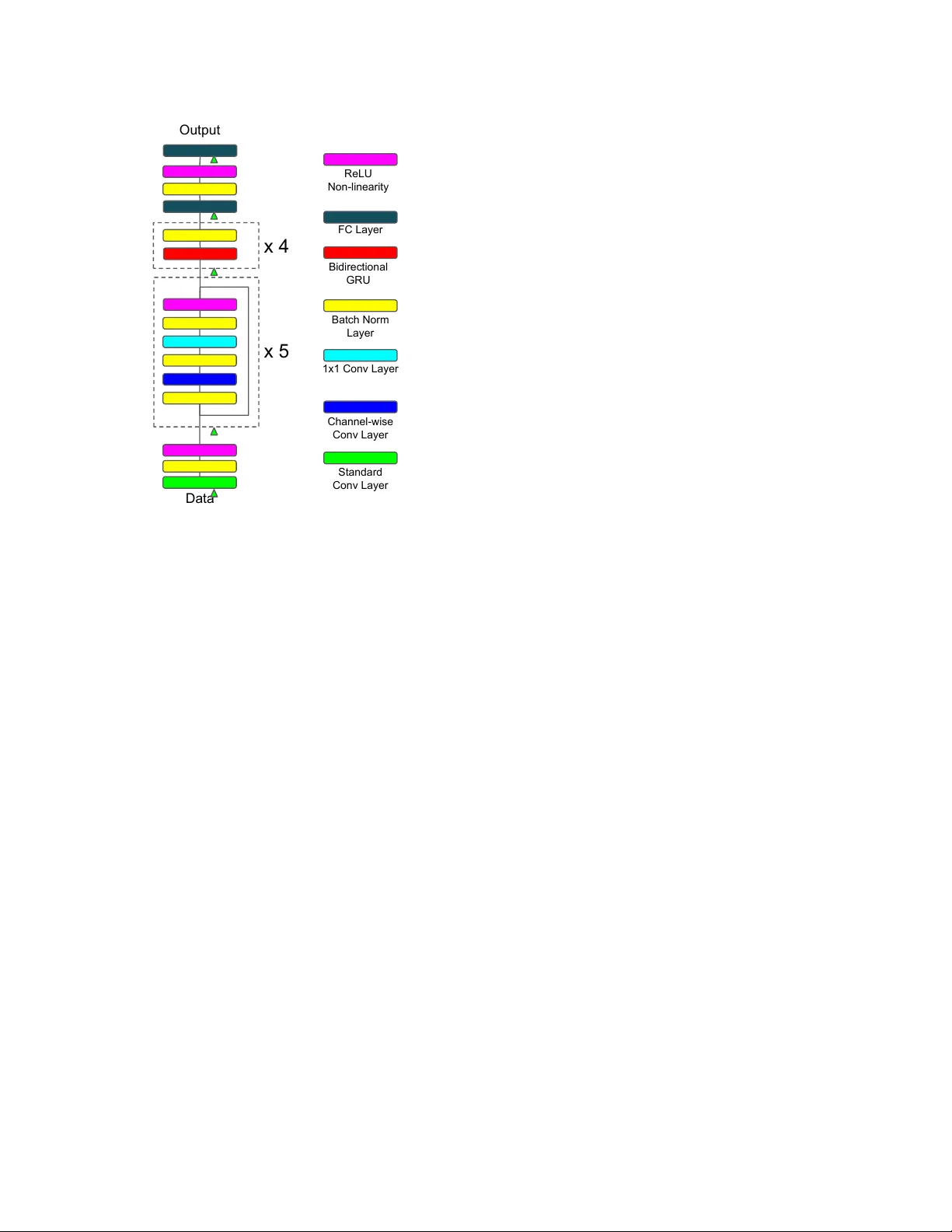
IMPR O VED REGULARIZA TION TECHNIQUES FOR END-TO-END SPEECH RECOGNITION Y ingbo Zhou, Caiming Xiong, Richar d Socher Salesforce Research ABSTRA CT Regularization is important for end-to-end speech models, since the models are highly flexible and easy to ov erfit. Data augmentation and dropout has been important for improv- ing end-to-end models in other domains. Howe v er , they are relativ ely under explored for end-to-end speech models. Therefore, we in vestig ate the effecti veness of both methods for end-to-end trainable, deep speech recognition models. W e augment audio data through random perturbations of tempo, pitch, v olume, temporal alignment, and adding random noise. W e further inv estigate the effect of dropout when applied to the inputs of all layers of the network. W e sho w that the combination of data augmentation and dropout giv e a rela- tiv e performance improvement on both W all Street Journal (WSJ) and LibriSpeech dataset of over 20% . Our model per- formance is also competitive with other end-to-end speech models on both datasets. Index T erms — regularization, data augmentation, deep learning, end-to-end speech recognition, dropout 1. INTR ODUCTION Regularization has proven crucial to improving the general- ization performance of many machine learning models. In particular , regularization is crucial when the model is highly flexible ( e.g. deep neural networks) and likely to overfit on the training data. Data augmentation is an ef ficient and ef- fectiv e w ay of doing regularization that introduces very small (or no) ov erhead during training. It has shown to consistently improv e performance in various pattern recognition tasks [1, 2, 3, 4, 5]. Dropout [6] is another powerful way of doing regularization for training deep neural networks, it intends to reduce the co-adaptation amongst hidden units by randomly zero-ing out inputs to the hidden layer during training. End-to-end speech models often ha ve millions of parame- ters [7, 8, 9, 10, 11]. Ho wev er , data augmentation and dropout hav e not been extensiv ely studied or applied to them. W e in- vestigate the effecti veness of data augmentation and dropout for regularizing end-to-end speech models. In particular , we augment the raw audio data by changing the tempo and pitch independently . The volume and temporal alignment of the au- dio signals are also randomly perturbed, with additional ran- dom noises added. T o further regularize the model, we em- ploy dropout to each input layer of the network. W ith these regularization techniques, we obtained ov er 20% relativ e per- formance on the W all Street Journal (WSJ) dataset and Lib- riSpeech dataset. 2. RELA TED WORK Data augmentation in speech recognition has been applied be- fore. Gales et al. [12] use hidden Markov models to gener- ate synthetic data to enable 1-vs-1 training of SVMs. Fea- ture lev el augmentation has also demonstrated effecti veness [5, 3, 4]. K o et al. [2] performed audio lev el speed pertur- bation that also lead to performance improvements. Back- ground noise is used for augmentation in [8, 9] to improve performance on noisy speech. Apart from adding noise, our data augmentation also modifies the tempo, pitch, volume and temporal alignment of the audio. Dropout has been applied to speech recognition before. It has been applied to acous- tic models in [13, 14, 15] and demonstrated promising per - formance. For end-to-end speech models, Hannun et al. [8] applied dropout to the output layer of the network. Howe ver , to the best of our knowledge, our work is the first to apply it to other layers in end-to-end speech models. 3. MODEL ARCHITECTURE The end-to-end model structure used in this work is very similar to the model architecture of Deep Speech 2 (DS2) [9]. While we hav e made some modifications at the front-end time-frequency con v olution ( i.e. 2-D con volution) layers, the core structure of recurrent layers is the same. The full end-to-end model structure is illustrated in Fig. 1. First, we use depth-wise separable conv olution [16, 17] for all the con volution layers. The performance adv antage of depth-wise separable con volution has been demonstrated in computer vision tasks [17] and is also more computation- ally ef ficient. The depth-wise separable con volution is im- plemented by first con volving over the input channel-wise. It then conv olves with 1 × 1 filters with the desired number of channels. Stride size only influence the channel-wise conv o- lution; the following 1 × 1 con volutions always hav e stride one. Second, we substitute normal con volution layers with Data Output x 5 x 4 Standard Conv Layer Channel-wise Conv Layer 1x1 Conv Layer Batch Norm Layer Bidirectional GRU FC Layer ReLU Non-linearity Fig. 1 . Model architecture of our end-to-end speech model. Different colored blocks represent dif ferent layers as shown on the right, the triangle indicates dropout happens right be- fore the pointed layer . ResNet [18] blocks. The residual connections help the gradi- ent flow during training. They ha ve been employed in speech recognition [11] and achieved promising results. For exam- ple, a w × h depth-wise separable conv olution with n input and m output channels is implemented by first con volving the input channel-wise with its corresponding w × h filters, fol- lowed by standard 1 × 1 con volution with m filters. Our model is composed of one standard con volution layer that has larger filter size, followed by fiv e residual con volu- tion blocks. Con volutional features are then giv en as input to a 4-layer bidirectional recurrent neural network with gated re- current units (GR U) [19]. Finally , two fully connected layers take the last hidden RNN layer as input and output the final per-character prediction. Batch normalization [20] is applied to all layers to facilitate training. 4. PREVENTING O VERFITTING Our model has ov er five million parameters (see sec. 5). This makes regularization important for it to generalize well. In this section we describe our primary methods for prev enting ov erfitting: data augmentation and dropout. 4.1. Data A ugmentation V ocal tract length perturbation (VTLP [5]) is a popular method for doing feature le vel data augmentation in speech. W e choose to do data lev el augmentation ( i.e. augment raw audio) instead of feature level augmentation, because the ab- sence of feature-level dependencies makes it more flexible. K o et al. [2] used data level augmentation and showed that modifying the speed of raw audio approximates the ef fect of VTLP and works better than VTLP . Howe ver , in speed perturbation since the pitch is positi vely correlated with the speed, it is not possible to generate audio with higher pitch but slo wer speed and vice versa. This may not be ideal, since it reduces the variation in the augmented data, which in turn may hurt performance. Therefore, T o get increased variation in our data, we separate the speed perturbation into two inde- pendent components – tempo and pitch. By keeping the pitch and tempo separate, we can cov er a wider range of variations. W e use the tempo and pitch functions from the SoX audio manipulation tool [21]. Generating noisy versions of the data is also a common way to do data augmentation. T o generate such data, we add random white noise to the audio signal. V olume of the audio is also randomly modified to simulate the effect of different recording volumes. T o further distort the audio, it is also ran- domly shifted by a small amount ( i.e. less than 10ms). With a combination of the above approaches, we can synthetically generate a lar ge amount of data that captures different varia- tions. 4.2. Dropout Dropout [6] is a po werful regularizer . It prev ents the co- adaptation of hidden units by randomly zero-ing out a sub- set of inputs for that layer during training. In more detail, let x t i ∈ R d denote the i -th input sample to a network layer at time t , dropout does the follo wing to the input during training z t ij ∼ Bernoulli (1 − p ) j ∈ { 1 , 2 , . . . , d } (1) ˆ x t i = x t i  z t i (2) where p is the dropout probability , z t i = [ z t i 1 , z t i 2 , . . . , z t id ] is the dropout mask for x t i , and  denote elementwise multi- plication. At test time, the input is rescaled by 1 − p so that the expected pre-activ ation stays the same as it was at train- ing time. This setup works well for feed forward networks in practice, ho wever , it hardly finds any success when applied to recurrent neural networks. Gal and Ghahramani [22] proposed a dropout variant that approximates a Bayesian neural network for recurrent net- works. The modification is principled and simple, i.e. instead of randomly drop different dimensions of the input across time, a fixed random mask is used for the input across time. More precisely , we modify the dropout to the input as fol- lows: 1 z ij ∼ Bernoulli (1 − p ) j ∈ { 1 , 2 , . . . , d } (3) ˆ x t i = x t i  z i (4) where z i = [ z i 1 , z i 2 , . . . , z id ] is the dropout mask. Since we are not interested in the Bayesian view of the model, we choose the same rescaling approximation as standard dropout ( i.e. rescale input by 1 − p ) instead of doing Monte Carlo approximation at test time. W e apply the dropout v ariant described in eq. 3 and 4 to inputs of all conv olutional and recurrent layers. Standard dropout is applied on the fully connected layers. 5. EXPERIMENTS T o in vestigate the ef fectiv eness of the proposed techniques, we perform experiments on the W all Street Journal (WSJ) and LibriSpeech [23] datasets. The input to the model is a spec- trogram computed with a 20ms window and 10ms step size. W e normalize each spectrogram to have zero mean and unit variance. In addition, we also normalize each feature to have zero mean and unit v ariance based on the training set statis- tics. No further preprocessing is done after these two steps of normalization. W e denote the size of the conv olution layer by tuple ( C, F , T , SF , ST ) , where C, F , T , SF , and ST denotes number of channels, filter size in frequency dimension, filter size in time dimension, stride in frequency dimension and stride in time dimension respectively . W e ha ve one con volutional layer with size (32,41,11,2,2), and five residual con volution blocks of size (32,7,3,1,1), (32,5,3,1,1), (32,3,3,1,1), (64,3,3,2,1), (64,3,3,1,1) respecti vely . Follo wing the con volutional lay- ers we hav e 4-layers of bidirectional GR U RNNs with 1024 hidden units per direction per layer . Finally we hav e one fully connected hidden layer of size 1024 followed by the output layer . The conv olutional and fully connected layers are initialized uniformly [24]. The recurrent layer weights are initialized with a uniform distrib ution U ( − 1 / 32 , 1 / 32) . The model is trained in an end-to-end fashion to maximize the log-likelihood using connectionist temporal classification [25]. W e use mini-batch stochastic gradient descent with batch size 64, learning rate 0.1, and with Nesterov momen- tum 0.95. The learning rate is reduced by half whenever the validation loss has plateaued, and the model is trained until the v alidation loss stops impro ving. The norm of the gradient is clipped [26] to have a maximum value of 1 . In addition, for all experiments we use l -2 weight decay of 1 e − 5 for all parameters. 1 In [22], the authors also have dropout applied on recurrent connections, we did not employ the recurrent dropout because dropout on the input is an easy drop-in substitution for cuDNN RNN implementation, whereas the recurrent one is not. Switch from cuDNN based RNN implementation will increase the computation time of RNNs by a significant amount, and thus we choose to av oid it. Regularization Methods eval92 Rel. Improv ement Baseline 8.38% – + Noise 7.88% 5.96% + T empo augmentation 7.02% 16.22% + All augmentation 6.63% 20.88% + Dropout 6.50% 22.43% + All regularization 6.42% 23.39% T able 1 . W ord error rate from WSJ dataset. Baseline de- notes model trained only with weight decay; noise denotes model trained with noise augmented data; tempo augmenta- tion denotes model trained with independent tempo and pitch perturbation; all augmentation denotes model trained with all proposed data augmentations; dropout denotes model trained with dropout. 5.1. Effect of individual regularizer T o study the effecti veness of data augmentation and dropout, we perform experiments on both datasets with v arious set- tings. The first set of e xperiments were carried out on the WSJ corpus. W e use the standard si284 set for training, dev93 for validation and eval92 for test ev aluation. W e use the pro- vided language model and report the result in the 20K closed vocab ulary setting with beam search. The beam width is set to 100. Since the training set is relati vely small ( ∼ 80 hours), we performed a more detailed ablation study on this dataset by separating the tempo based augmentation from the one that generates noisy versions of the data. For tempo based data augmentation, the tempo parameter is selected follow- ing a uniform distribution U (0 . 7 , 1 . 3) , and U ( − 500 , 500) for pitch. Since WSJ has relativ ely clean recordings, we k eep the signal to noise ratio between 10 and 15db when adding white noise. The gain is selected from U ( − 20 , 10) and the audio is shifted randomly by 0 to 10ms. Results are sho wn in T able 1. Both approaches improve the performance over the baseline, where none of the additional regularization is applied. Noise augmentation has demonstrated its effecti veness for making the model more robust against noisy inputs. W e show here that adding a small amount of noise also benefits the model on relati vely clean speech samples. T o compare with exist- ing augmentation methods,we trained a model by using speed perturbation. W e use 0.9, 1.0, and 1.1 as the perturb coeffi- cient for speed as suggested in [2]. This results in a WER of 7.21%, which brings 13.96% relativ e performance improve- ment. Our tempo based augmentation is slightly better than the speed augmentation, which may attrib ute to more vari- ations in the augmented data. When the techniques for data augmentation are combined, we ha ve a significant relative im- prov ement of 20% over the baseline (see table 1). Dropout also significantly improv ed the performance ( 22% relativ e improv ement, see table 1). The dropout proba- bilities are set as follows, 0 . 1 for data, 0 . 2 for all con volution (a) (b) Fig. 2 . T raining and validation loss on WSJ dataset, where a) sho ws the learning curve from the baseline model, and b) shows the loss when re gularizations are applied. Regularization test-clean test-other Methods Baseline 7.45% 22.59% + All augmentation 6.31% (15.30%) 18.59% (17.70%) + Dropout 5.87% (21.20%) 17.08% (24.39%) + All regularization 5.67% (23.89%) 15.18% (32.80%) T able 2 . W ord error rate on the Librispeech dataset, num- bers in parenthesis indicate relative performance improve- ment ov er baseline. Notations are the same as in table 1. layers, 0 . 3 for all recurrent and fully connected layers. By combining all regularization, we achiev e a final WER of 6 . 42% . Fig. 2 shows the training curve of baseline and reg- ularized models. It is clear that with regularization, the gap between the v alidation and training loss is narro wed. In addi- tion, the re gularized training also results in a lo wer validation loss. W e also performed experiments on the LibriSpeech dataset. The model is trained using all 960 hours of train- ing data. W e use both dev-clean and dev-other for validation and report results on test-clean and test-other . The provided 4-gram language model is used for final beam search decod- ing. The beam width used in this experiment is also set to 100. The results follow a similar trend as the previous exper - iments. W e achieved relativ e performance improv ement of ov er 22% on test-clean and over 32% on test-other set (see table 2). 5.2. Comparison to other methods In this section, we compare our end-to-end model with other end-to-end speech models. The results from WSJ and Lib- riSpeech (see table 3 and 4) are obtained through beam search decoding with the language model provided with the dataset with beam size 100. T o make a fair comparison on the WSJ corpus, we additionally trained an e xtended trigram model Method Eval 92 Bahdanau et al. [10] 9.30% Grav es and Jaitly [27] 8.20% Miao et al. [7] 7.34% Ours 6.42% Ours (extended 3-gram) 6.26% Amodei et al. [9] 3.60% T able 3 . W ord error rate comparison with other end-to-end methods on WSJ dataset. Method test-clean test-other Collobert et al. [28] 7.20% - ours 5.67% 15.18% Amodei et al. [9] 5.33% 13.25% T able 4 . W ord error rate comparison with other end-to-end methods on LibriSpeech dataset. with the data released with the corpus. Our results on both WSJ and LibriSpeech are competitiv e to e xisting methods. W e would like to note that our model achie ved comparable re- sults with Amodei et al. [9] on LibriSpeech dataset, although our model is only trained only on the provided training set. This demonstrates the effecti veness of the proposed regular - ization methods for training end-to-end speech models. 6. CONCLUSION In this paper, we in vestigate the ef fectiv eness of data augmen- tation and dropout for deep neural network based, end-to-end speech recognition models. F or data augmentation, we inde- pendently v ary the tempo and pitch of the audio so that it is able to generate a large variety of additional data. In addition, we also add noisy versions of the data by changing the gain, shifting the audio, and add random white noise. W e show that, with tempo and noise based augmentation, we are able to achiev e 15–20% relativ e performance improvement on WSJ and LibriSpeech dataset. W e further in vestigate the regular- ization of dropout by applying it to inputs of all layers of the network. Similar to data augmentation, we obtained signif- icant performance improvements. When both regularization techniques are combined, we achie ved ne w state-of-the-art re- sults on both dataset, with 6.26% on WSJ, and 5.67% and 15.18% on test-clean and test-other set from LibriSpeech. 7. REFERENCES [1] A. Krizhevsk y , I. Sutske ver , and G. E. Hinton, “Ima- genet classification with deep con volutional neural net- works, ” in Advances in Neural Information Pr ocessing Systems , 2012, pp. 1106–1114. [2] T . Ko, V . Peddinti, D. Pove y , and S. Khudanpur , “ Au- dio augmentation for speech recognition., ” in INTER- SPEECH , 2015, pp. 3586–3589. [3] X. Cui, V . Goel, and B. Kingsb ury , “Data augmentation for deep neural network acoustic modeling, ” in ICASSP , May 2014, pp. 5582–5586. [4] X. Cui, V . Goel, and B. Kingsb ury , “Data augmentation for deep conv olutional neural network acoustic model- ing, ” in ICASSP , April 2015, pp. 4545–4549. [5] N. Jaitly and G. E Hinton, “V ocal tract length pertur- bation (vtlp) improves speech recognition, ” in ICML W orkshop , 2013, pp. 625–660. [6] Nitish Sri vasta va, Geoffre y Hinton, Ale x Krizhevsk y , Ilya Sutske ver , and Ruslan Salakhutdinov , “Dropout: A simple way to pre vent neural networks from overfit- ting, ” The Journal of Machine Learning Resear ch , vol. 15, no. 1, pp. 1929–1958, 2014. [7] Y Miao, M Gow ayyed, and F Metze, “Eesen: End-to- end speech recognition using deep rnn models and wfst- based decoding, ” in ASR U . IEEE, 2015, pp. 167–174. [8] A. Hannun, C. Case, J. Casper , B. Catanzaro, G. Di- amos, E. Elsen, R. Prenger , S. Satheesh, S. Sengupta, A. Coates, et al., “Deep speech: Scaling up end-to-end speech recognition, ” arXiv pr eprint arXiv:1412.5567 , 2014. [9] D. Amodei, S. Ananthanarayanan, R. Anubhai, J. Bai, E. Battenberg, C. Case, J. Casper , B. Catanzaro, Q. Cheng, G. Chen, et al., “Deep speech 2: End-to-end speech recognition in english and mandarin, ” in ICML , 2016, pp. 173–182. [10] D Bahdanau, J Choro wski, D Serdyuk, P Brakel, and Y Bengio, “End-to-end attention-based large vocabulary speech recognition, ” in ICASSP . IEEE, 2016, pp. 4945– 4949. [11] Y Zhang, W Chan, and N Jaitly , “V ery deep con volu- tional networks for end-to-end speech recognition, ” in ICASSP . IEEE, 2017, pp. 4845–4849. [12] M. JF Gales, A. Ragni, H AlDamarki, and C Gau- tier , “Support vector machines for noise robust asr , ” in ASR U . IEEE, 2009, pp. 205–210. [13] G E Dahl, T N Sainath, and G E Hinton, “Improv- ing deep neural networks for lvcsr using rectified linear units and dropout, ” in ICASSP . IEEE, 2013, pp. 8609– 8613. [14] T N Sainath, B Kingsbury , G Saon, H Soltau, A Mo- hamed, G Dahl, and B Ramabhadran, “Deep con vo- lutional neural networks for large-scale speech tasks, ” Neural Networks , vol. 64, pp. 39–48, 2015. [15] G Saon, HK J K uo, S Rennie, and M Picheny , “The ibm 2015 english conv ersational telephone speech recogni- tion system, ” arXiv pr eprint arXiv:1505.05899 , 2015. [16] L Sifre and S Mallat, “Rotation, scaling and deforma- tion inv ariant scattering for texture discrimination, ” in CVPR , 2013, pp. 1233–1240. [17] F Chollet, “Xception: Deep learning with depth- wise separable con volutions, ” arXiv pr eprint arXiv:1610.02357 , 2016. [18] K He, X Zhang, S Ren, and J Sun, “Deep residual learn- ing for image recognition, ” in CVPR , 2016, pp. 770– 778. [19] K Cho, Bart V an M, D Bahdanau, and Y Bengio, “On the properties of neural machine translation: Encoder- decoder approaches, ” arXiv pr eprint arXiv:1409.1259 , 2014. [20] S Ioffe and C Szegedy , “Batch normalization: Acceler - ating deep netw ork training by reducing internal cov ari- ate shift., ” in ICML , Francis R. Bach and David M. Blei, Eds. 2015, vol. 37 of JMLR Pr oceedings , pp. 448–456, JMLR.org. [21] “Sound exchange, ” http://sox.sourceforge. net . [22] Y Gal and Z Ghahramani, “ A theoretically grounded application of dropout in recurrent neural networks, ” in NIPS , 2016, pp. 1019–1027. [23] V Panayoto v , G Chen, D Pove y , and S Khudanpur , “Lib- rispeech: an asr corpus based on public domain audio books, ” in ICASSP . IEEE, 2015, pp. 5206–5210. [24] K He, X Zhang, S Ren, and J Sun, “Delving deep into rectifiers: Surpassing human-le vel performance on im- agenet classification, ” in Pr oceedings of the IEEE in- ternational confer ence on computer vision , 2015, pp. 1026–1034. [25] A. Grav es, S. Fern ´ andez, F . Gomez, and J. Schmidhuber, “Connectionist temporal classification: labelling unseg- mented sequence data with recurrent neural networks, ” in ICML . A CM, 2006, pp. 369–376. [26] R Pascanu, T Mikolov , and Y Bengio, “On the difficulty of training recurrent neural networks, ” in ICML , 2013, pp. 1310–1318. [27] A Graves and N Jaitly , “T owards end-to-end speech recognition with recurrent neural networks, ” in ICML , 2014, pp. 1764–1772. [28] R Collobert, C Puhrsch, and G Synnaeve, “W av2letter: an end-to-end con vnet-based speech recognition sys- tem, ” arXiv pr eprint arXiv:1609.03193 , 2016.