Improving End-to-End Speech Recognition with Policy Learning

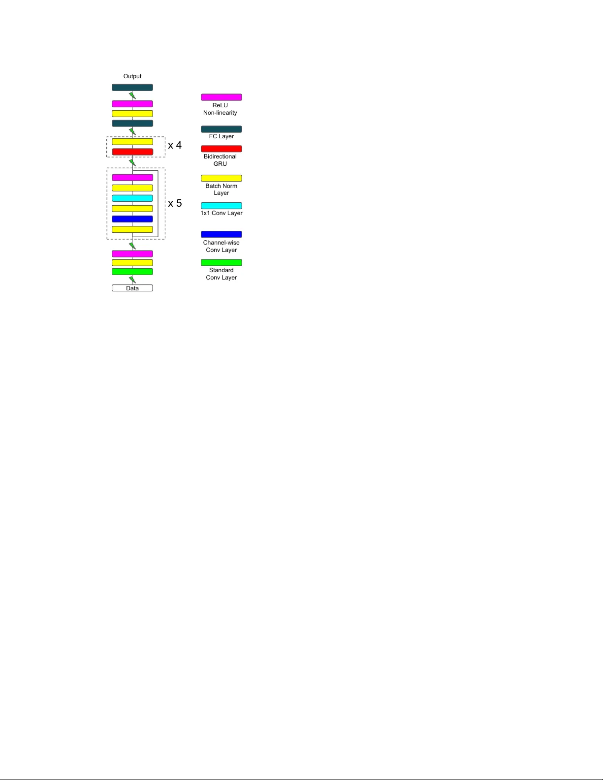
IMPR O VING END-TO-END SPEECH RECOGNITION WITH POLICY LEARNING Y ingbo Zhou, Caiming Xiong, Richar d Socher Salesforce Research ABSTRA CT Connectionist temporal classification (CTC) is widely used for maximum likelihood learning in end-to-end speech recog- nition models. Howe ver , there is usually a disparity between the negativ e maximum likelihood and the performance met- ric used in speech recognition, e .g. , word error rate (WER). This results in a mismatch between the objecti ve function and metric during training. W e show that the above problem can be mitigated by jointly training with maximum likelihood and policy gradient. In particular, with polic y learning we are able to directly optimize on the (otherwise non-differentiable) per- formance metric. W e show that joint training improves rela- tiv e performance by 4% to 13% for our end-to-end model as compared to the same model learned through maximum like- lihood. The model achie ves 5.53% WER on W all Street Jour- nal dataset, and 5.42% and 14.70% on Librispeech test-clean and test-other set, respectiv ely . Index T erms — end-to-end speech recognition, L VCSR, policy gradient, deep neural networks 1. INTR ODUCTION Deep neural networks are the basis for some of the most ac- curate speech recognition systems in research and production [1, 2, 3]. Neural network based acoustic models are com- monly used as a sub-component in a Gaussian mixture model (GMM) and hidden Markov model (HMM) based hybrid sys- tem. Alignment is necessary to train the acoustic model, and a two-stage ( i.e. alignment and frame prediction) training pro- cess is required for a typical hybrid system. A drawback of such setting is that there is a disconnect between the acous- tic model training and the final objective, which makes the system lev el optimization dif ficult. The end-to-end neural network based speech models by- pass this two-stage training process by directly maximizing the likelihood of the data. More recently , the end-to-end mod- els have also shown promising results on various datasets [4, 5, 6, 7]. While the end-to-end models are commonly trained with maximum likelihood, the final performance metric for a speech recognition system is typically w ord error rate (WER) or character error rate (CER). This results a mismatch be- tween the objective that is optimized and the ev aluation met- ric. In an ideal setting the model should be trained to optimize the final metric. Howe ver , since the metrics are commonly discrete and non-differentiable, it is very difficult to optimize them in practice. Lately , reinforcement learning (RL) has shown to be ef- fectiv e on improving performance for problems that hav e non-differentiable metric through policy gradient. Promis- ing results are obtained in machine translation [8, 9], image captioning [8, 10], summarization [8, 11], etc. . In particu- lar , REINFORCE algorithm [12] enables one to estimate the gradient of the expected re ward by sampling from the model. It has also been applied for online speech recognition [13]. Grav es and Jaitly [4] propose expected transcription loss that can be used to optimize on WER. Howe ver , it is more com- putationally e xpensive. For example, for a sequence of length T with vocabulary size K , at least T samples and K metric calculations are required for estimating the loss. W e sho w that jointly training end-to-end models with self critical sequence training (SCST) [10] and maximum likeli- hood improv es performance significantly . SCST is also effi- cient during training, as only one sampling process and two metric calculations are necessary . Our model achie ves 5.53% WER on W all Street Journal dataset, and 5.42% and 14.70% WER on Librispeech test-clean and test-other sets. 2. MODEL STR UCTURE The end-to-end model structure used in this work is very simi- lar to that of Deep Speech 2 (DS2) [6]. It is mainly composed of 1) a stack of con volution layers in the front-end for fea- ture extraction, and 2) a stack of recurrent layers for sequence modeling. The structure of recurrent layers is the same as in DS2, and we illustrate the modifications in con volution layers in this section. W e choose to use time and frequency conv olution ( i.e. 2- D con volution) as the front-end of our model, since it is able to model both the temporal transitions and spectral v ariations in speech utterances. W e use depth-wise separable conv olu- tion [14, 15] for all the con volution layers, due to its computa- tional ef ficiency and performance adv antage [15]. The depth- wise separable conv olution is implemented by first con volv- ing o ver the input channel-wise, and then con volve with 1 × 1 filters with the desired number of output channels. Stride size only influences the channel-wise con volution; the following 1 × 1 con volutions alw ays have stride size of one. More pre- Data Output x 5 x 4 Standard Conv Layer Channel-wise Conv Layer 1x1 Conv Layer Batch Norm Layer Bidirectional GRU FC Layer ReLU Non-linearity Fig. 1 . Model architecture of our end-to-end speech model. Different colored blocks represent different layers as shown on the right, the lightning symbol indicates dropout happens between the two layers. cisely , let x ∈ R F × T × D , c ∈ R W × H × D and w ∈ R D × N denote an input sample, the channel-wise con volution and the 1 × 1 con volution weights respecti vely . The depth-wise sepa- rable conv olution with D input channels and N output chan- nels performs the following operations: s ( i, j, d ) = F − 1 X f =0 T − 1 X t =0 x ( f , t, d ) c ( i − f , j − t, d ) (1) o ( i, j, n ) = D − 1 X k =0 s ( i, j, k ) w ( k , n ) (2) where d ∈ { 1 , . . . , D } and n ∈ { 1 , 2 , . . . , N } , s is the channel-wise con volution result, and o is the result from depth-wise separable conv olution. In addition, we add a residual connection [16] between the input and the layer output for the depth-wise separable con volution to facilitate training. Our model is composed of six con volution layers – one standard con volution layer that has larger filter size, follo wed by five residual con volution blocks [16]. The conv olution fea- tures are then fed to four bidirectional gated recurrent units (GR U) [17] layers, and finally two fully connected layers that make the final per-character prediction. The full end-to-end model structure is illustrated in Fig. 1. 3. MODEL OBJECTIVE 3.1. Maximum Likelihood T raining Connectionist temporal classification (CTC) [18] is a popular method for doing maximum likelihood training on sequence labeling tasks, where the alignment information is not pro- vided in the label. The alignment is not required since CTC marginalizes o ver all possible alignments, and maximizes the likelihood P ( y | x ) . It achie ves this by augmenting the orig- inal label set L to set Ω = L ∪ { blank } with an additional blank symbol. A mapping M is then defined to map a length T sequence of label Ω T to L ≤ T by removing all blanks and repeated symbols along the path. The likelihood can then be recov ered by P ( y 0 | x ) = Y t P ( y 0 t | x ) , y 0 t ∈ Ω T P ( y | x ) = X y 0 ∈M − 1 ( y ) P ( y 0 | x ) where x , y and y 0 denote an input example of length T , the corresponding label of length ≤ T and one of the augmented label with length T . 3.2. Policy Learning The log likelihood reflects the log probability of getting the whole transcription completely correct. What it ignores are the probabilities of the incorrect transcriptions. In other words, all incorrect transcriptions are equally bad, which is clearly not the case. Furthermore, the performance metrics typically aim to reflect the plausibility of incorrect predic- tions. For example, WER penalizes less for transcription that has less edit distance to the ground truth label. This results in a disparity between the optimization objecti ve of the model and the (commonly discrete) e valuation criteria. This mis- match is mainly attrib uted to the inability to directly optimize the criteria. One way to remedy this mismatch is to view the above problem in the policy learning frame work. In this frame work, we can view our model as an agent and the training samples as the envir onment . The parameters of the model θ defines a pol- icy P θ ( y | x ) , the model interacts with the environment by fol- lowing this policy . The agent then performs an action based on its current state , in which case the action is the generated transcription and the state is the model hidden representation of the data. It then observes a r ewar d that is defined from the ev aluation metric calculated on the current sample ( e.g. 1 − WER for the current transcription). The goal of learning is to obtain a policy that minimizes the negati ve expected re- ward: L p ( θ ) = − E y s ∼ P θ ( y | x ) [ r ( y s )] (3) where r ( · ) denotes the re ward function. Gradient of eq. 3 can be obtained through REINFORCE [12] as ∇ θ L p ( θ ) = − E y s ∼ P θ ( y | x ) [ r ( y s ) ∇ θ log P θ ( y s | x )] (4) ≈ − r ( y s ) ∇ θ log P θ ( y s | x ) (5) Eq. 5 shows the Monte Carlo approximation of the gradi- ent with a single example, which is a common practice when training model with stochastic gradient descent. The policy gradient obtained from eq. 5 is often of high variance, and the training can get unstable. T o reduce the variance, Rennie et al. [10] proposed self-critical sequence training (SCST). In SCST , the policy gradient is computed with a baseline , which is the greedy output from the model. Formally , the policy gradient is calculated using ∇ θ L p ( θ ) = − E y s ∼ P θ ( y | x ) [( r ( y s ) − r ( ˆ y )) ∇ θ log P θ ( y s | x )] (6) ≈ − ( r ( y s ) − r ( ˆ y )) ∇ θ log P θ ( y s | x ) (7) where ˆ y is the greedy decoding output from the model for the input sample x . 3.3. Multi-objective Policy Learning A potential problem with policy gradient methods (including SCST) is that the learning can be slo w and unstable at the be- ginning of training. This is because it is unlikely for the model to ha ve reasonable output at that stage, which leads to im- plausible samples with lo w rew ards. Learning will be slo w in case of small learning rate, and unstable otherwise. One way to remedy this problem is to incorporate maximum likelihood objectiv e along with policy gradient, since in maximum like- lihood the probability is e valuated on the ground truth tar gets, and hence will get large gradients when the model output is incorrect. This leads to the following objecti ve for training our end-to-end speech model: L ( θ ) = − log P θ ( y | x ) + λL scst ( θ ) where (8) L scst ( θ ) = − { g ( y s , y ) − g ( ˆ y , y ) } log P θ ( y s | x ) where g ( · , · ) is the re ward function and λ ∈ (0 , + ∞ ) is the coefficient that controls the contribution from SCST . In our case we choose g ( · , y ) = 1 − max(1 , WER ( · , y )) . Training with eq. 8 is also efficient, since both sampling and greedy decoding is cheap. The only place that might be computation- ally more demanding is the rew ard calculation, howe ver , we only need to compute it twice per batch of e xamples, which adds only a minimal ov erhead. 4. EXPERIMENTS W e ev aluate the proposed objective by performing experi - ments on the W all Street Journal (WSJ) and LibriSpeech [19] datasets. The input to the model is a spectrogram computed with a 20ms window and 10ms step size. W e first normalize each spectrogram to hav e zero mean and unit v ariance. In ad- dition, we also normalize each feature to hav e zero mean and unit v ariance based on the training set statistics. No further preprocessing is done after these two steps of normalization. W e denote the size of the con volution layer by the tuple ( C, F , T , SF , ST ) , where C, F , T , SF , and ST denote number of channels, filter size in frequency dimension, filter size in time dimension, stride in frequency dimension and stride in time dimension respecti vely . W e hav e one con volutional layer with size (32,41,11,2,2), and five residual con volution blocks of size (32,7,3,1,1), (32,5,3,1,1), (32,3,3,1,1), (64,3,3,2,1), (64,3,3,1,1) respectiv ely . Follo wing the conv olutional layers we have 4 layers of bidirectional GRU RNNs with 1024 hid- den units per direction per layer . Finally , we ha ve one fully connected hidden layer of size 1024 follo wed by the output layer . Batch normalization [20] is applied to all layers’ pre- activ ations to facilitate training. Dropout [21] is applied to inputs of each layer , and for layers that take sequential input ( i.e. the conv olution and recurrent layers) we use the dropout variant proposed by Gal and Ghahramani [22]. The con vo- lutional and fully connected layers are initialized uniformly following He et al. [23]. The recurrent layer weights are initialized with a uniform distribution U ( − 1 / 32 , 1 / 32) . The model is trained in an end-to-end fashion to minimize the mixed objectiv e as illustrated in eq. 8. W e use mini-batch stochastic gradient descent with batch size 64, learning rate 0.1, and with Nesterov momentum 0.95. The learning rate is reduced by half whene ver the v alidation loss has plateaued. W e set λ = 0 . 1 at the be ginning of training, and increase it to 1 after the model has con ver ged ( i.e. the validation loss stops improving). The gradient is clipped [24] to hav e a maximum ` 2 norm of 1 . For regularization, we use ` 2 weight decay of 10 − 5 for all parameters. Additionally , we apply dropout for inputs of each layer (see Fig. 1). The dropout probabilities are set as 0 . 1 for data, 0 . 2 for all conv olution layers, and 0 . 3 for all recurrent and fully connected layers. Furthermore, we also augment the audio training data through random pertur- bations of tempo, pitch, volume, temporal alignment, along with adding random noise. 4.1. Effect of Policy Learning T o study the ef fectiveness of our multi-objecti ve polic y learn- ing, we perform experiments on both datasets with v arious settings. The first set of experiments was carried out on the WSJ corpus. W e use the standard si284 set for training, dev93 for validation and eval92 for test ev aluation. W e use the pro- vided language model and report the result in the 20K closed vocab ulary setting with beam search. The beam width is set to 100. Results are sho wn in table 1. Both policy gradient methods improve results over baseline. In particular , the use of SCST results in 13.8% relative performance improvement on the eval92 set over the baseline. On LibriSpeech dataset, the model is trained using all 960 Method dev93 ev al92 CER WER CER WER Baseline 4.07% 9.93% 2.59% 6.42% Policy (eq. 5) 3.71% 9.46% 2.31% 5.85% Policy (eq. 7) 3.52% 9.21% 2.10% 5.53% T able 1 . Performance from WSJ dataset. Baseline denotes model trained without CTC only; policy indicates model trained using the multi-objectiv e policy learning. Equation in parenthesis indicates the way used to obtain policy gradient. Dataset Baseline Policy dev-clean CER 1.76% 1.69% WER 5.33% 5.10% test-clean CER 1.87% 1.75% WER 5.67% 5.42% dev-other CER 6.60% 6.26% WER 14.88% 14.26% test-other CER 6.58% 6.25% WER 15.18% 14.70% T able 2 . Performance from LibriSpeech dataset. Policy de- notes model trained with multi-objectiv e shown in eq. 8. Method WER Hannun et al. [25] 14.10 % Bahdanau et al. [7] 9.30% Grav es and Jaitly [4] 8.20% W u et al. [26] 8.20% Miao et al. [5] 7.34% Chorowski and Jaitly [27] 6.70% Human [6] 5.03% Amodei et al. [6]* 3.60% Ours 5.53% Ours (LibriSpeech) 4.67% T able 3 . Comparative results with other end-to-end methods on WSJ eval92 dataset. LibriSpeech denotes model trained using LibriSpeech dataset only , and test on WSJ. Amodei et al. used more training data. hours of training data. Both dev-clean and de v-other are used for validation and results are reported in table 2. The provided 4-gram language model is used for final beam search decod- ing. The beam width is also set to 100 for decoding. Overall, a relativ e ≈ 4% performance improvement over the baseline is observed. Method test-clean test-other Collobert et al. [28] 7.20% - Amodei et al. [6]* 5.33% 13.25% ours 5.42% 14.70% T able 4 . W ord error rate comparison with other end-to-end methods on LibriSpeech dataset. Amodei et al. used more training data. 4.2. Comparison with Other Methods W e also compare our performance with other end-to-end models. Comparati ve results from WSJ and LibriSpeech dataset are illustrated in tables 3 and 4 respectively . Our model achie ved competiti ve performance with other meth- ods on both datasets. In particular, with the help of policy learning we achieved similar results as Amodei et al. [6] on LibriSpeech without using additional data. T o see if the model generalizes, we also tested our LibriSpeech model on the WSJ dataset. The result is significantly better than the model trained on WSJ data (see table 3), which suggests that the end-to-end models benefit more when more data is av ailable. 5. CONCLUSION In this work, we try to close the gap between the maximum likelihood training objecti ve and the final performance metric for end-to-end speech models. W e sho w this gap can be re- duced by using the policy gradient method along with the neg- ativ e log-likelihood. In particular , we apply a multi-objectiv e training with SCST to reduce the expected negati ve reward that is defined by using the final metric. The joint training is computationally efficient. W e sho w that the joint training is effecti ve even with single sample approximation, which im- prov es the relative performance on WSJ and LibriSpeech by 13% and 4% ov er the baseline. 6. REFERENCES [1] G Hinton, L Deng, D Y u, G E Dahl, A Mohamed, N Jaitly , A Senior , V V anhoucke, P Nguyen, T Sainath, et al., “Deep neural networks for acoustic modeling in speech recognition: The shared views of four research groups, ” IEEE Signal Processing Magazine , v ol. 29, no. 6, pp. 82–97, 2012. [2] G Saon, HK J K uo, S Rennie, and M Picheny , “The ibm 2015 english con versational telephone speech recogni- tion system, ” arXiv preprint , 2015. [3] W Xiong, J Droppo, X Huang, F Seide, M Seltzer , A Stolcke, D Y u, and G Zweig, “The microsoft 2016 con versational speech recognition system, ” in Acous- tics, Speech and Signal Processing (ICASSP), 2017 IEEE International Conference on . IEEE, 2017, pp. 5255–5259. [4] A Gra ves and N Jaitly , “T ow ards end-to-end speech recognition with recurrent neural networks, ” in ICML , 2014, pp. 1764–1772. [5] Y Miao, M Gowayyed, and F Metze, “Eesen: End-to- end speech recognition using deep rnn models and wfst- based decoding, ” in ASR U . IEEE, 2015, pp. 167–174. [6] D. Amodei, S. Ananthanarayanan, R. Anubhai, J. Bai, E. Battenberg, C. Case, J. Casper , B. Catanzaro, Q. Cheng, G. Chen, et al., “Deep speech 2: End-to-end speech recognition in english and mandarin, ” in ICML , 2016, pp. 173–182. [7] D Bahdanau, J Chorowski, D Serdyuk, P Brakel, and Y Bengio, “End-to-end attention-based large v ocabulary speech recognition, ” in ICASSP . IEEE, 2016, pp. 4945– 4949. [8] M Ranzato, S Chopra, M Auli, and W Zaremba, “Se- quence le vel training with recurrent neural networks, ” arXiv pr eprint arXiv:1511.06732 , 2015. [9] D Bahdanau, P Brakel, K Xu, A Goyal, R Lo we, J Pineau, A Courville, and Y Bengio, “ An actor- critic algorithm for sequence prediction, ” arXiv pr eprint arXiv:1607.07086 , 2016. [10] S J Rennie, E Marcheret, Y Mroueh, J Ross, and V Goel, “Self-critical sequence training for image captioning, ” arXiv pr eprint arXiv:1612.00563 , 2016. [11] R Paulus, C Xiong, and R Socher , “ A deep reinforced model for abstracti ve summarization, ” arXiv preprint arXiv:1705.04304 , 2017. [12] R J Williams, “Simple statistical gradient-following al- gorithms for connectionist reinforcement learning, ” Ma- chine learning , vol. 8, no. 3-4, pp. 229–256, 1992. [13] Y Luo, C Chiu, N Jaitly , and I Sutske ver , “Learning online alignments with continuous rewards policy gra- dient, ” in ICASSP . IEEE, 2017, pp. 2801–2805. [14] L Sifre and S Mallat, “Rotation, scaling and deforma- tion inv ariant scattering for texture discrimination, ” in CVPR , 2013, pp. 1233–1240. [15] F Chollet, “Xception: Deep learning with depth- wise separable con volutions, ” arXiv pr eprint arXiv:1610.02357 , 2016. [16] K He, X Zhang, S Ren, and J Sun, “Deep residual learn- ing for image recognition, ” in CVPR , 2016, pp. 770– 778. [17] K Cho, Bart V an M, D Bahdanau, and Y Bengio, “On the properties of neural machine translation: Encoder- decoder approaches, ” arXiv pr eprint arXiv:1409.1259 , 2014. [18] A Grav es, S Fern ´ andez, F Gomez, and J Schmidhuber , “Connectionist temporal classification: labelling unseg- mented sequence data with recurrent neural networks, ” in ICML . A CM, 2006, pp. 369–376. [19] V Panayotov , G Chen, D Pove y , and S Khudanpur , “Lib- rispeech: an asr corpus based on public domain audio books, ” in ICASSP . IEEE, 2015, pp. 5206–5210. [20] S Ioffe and C Szegedy , “Batch normalization: Acceler- ating deep netw ork training by reducing internal cov ari- ate shift., ” in ICML , Francis R. Bach and Da vid M. Blei, Eds. 2015, vol. 37 of JMLR Pr oceedings , pp. 448–456, JMLR.org. [21] N Sriv astav a, G Hinton, A Krizhevsky , I Sutskev er , and R Salakhutdinov , “Dropout: A simple way to pre vent neural networks from overfitting, ” The Journal of Ma- chine Learning Researc h , v ol. 15, no. 1, pp. 1929–1958, 2014. [22] Y Gal and Z Ghahramani, “ A theoretically grounded application of dropout in recurrent neural networks, ” in NIPS , 2016, pp. 1019–1027. [23] K He, X Zhang, S Ren, and J Sun, “Delving deep into rectifiers: Surpassing human-lev el performance on im- agenet classification, ” in Pr oceedings of the IEEE in- ternational confer ence on computer vision , 2015, pp. 1026–1034. [24] R Pascanu, T Mikolo v , and Y Bengio, “On the difficulty of training recurrent neural networks, ” in ICML , 2013, pp. 1310–1318. [25] A Hannun, A Maas, D Jurafsk y , and A Ng, “First- pass large vocab ulary continuous speech recognition using bi-directional recurrent dnns, ” arXiv preprint arXiv:1408.2873 , 2014. [26] Y W u, S Zhang, Y Zhang, Y Bengio, and R Salakhutdi- nov , “On multiplicati ve integration with recurrent neural networks, ” in NIPS , 2016, pp. 2856–2864. [27] J Chorowski and N Jaitly , “T ow ards better decoding and language model integration in sequence to sequence models, ” arXiv preprint , 2016. [28] R Collobert, C Puhrsch, and G Synnaev e, “W av2letter: an end-to-end convnet-based speech recognition sys- tem, ” arXiv preprint , 2016.