Identifying the Mislabeled Training Samples of ECG Signals using Machine Learning

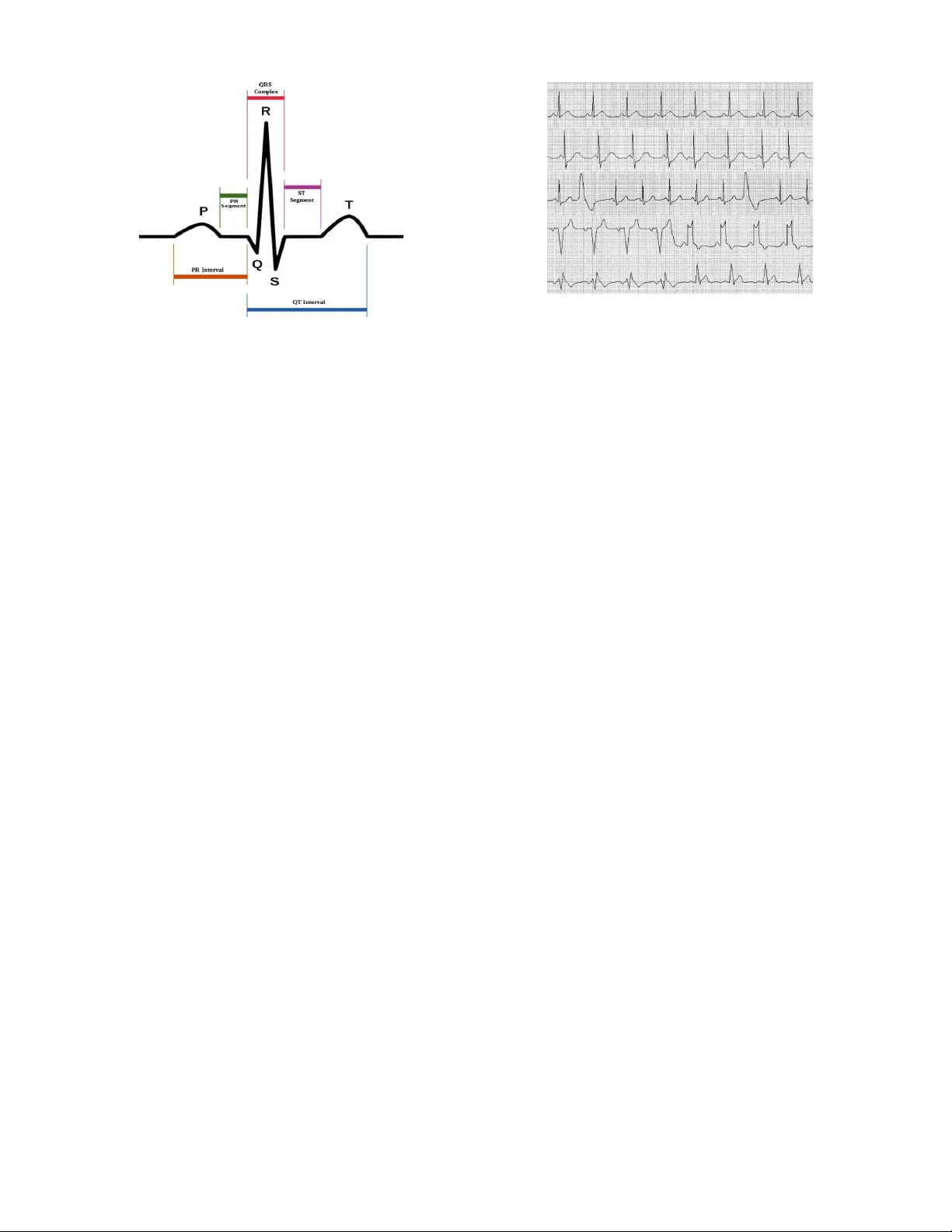
SUBMITTED TO IEEE JOURN AL OF BIOMEDICAL AND HEAL TH INFORMA TICS 1 Identifying the Mislabeled T raining Samples of ECG Signals using Machine Learning Y aoguang Li, W ei Cui Senior Member , IEEE and Cong W ang Senior Member , IEEE Abstract —The classification accuracy of electrocardiogram signal is often affected by diverse factors in which mislabeled training samples issue is one of the most influential problems. In order to mitigate this negative effect, the method of cross validation is introduced to identify the mislabeled samples. The method utilizes the cooperative advantages of different classifiers to act as a filter for the training samples. The filter removes the mislabeled training samples and retains the correctly labeled ones with the help of 10-f old cross validation. Consequently , a new training set is pro vided to the final classifiers to acquire higher classification accuracies. Finally , we numerically show the effectiveness of the proposed method with the MIT -BIH arrhythmia database. Index T erms —ECG signal, mislabeled samples, cross valida- tion, machine learning . I . I N T RO D U C T I O N C ARDIA C disease has become a key issue that threatens human life safety . How to detect heart disease as early as possible is the core of this problem, because cardiac disease is very prone to sudden death, which mak es the detection of heart disease more urgent than treatment. Electrocardiogram (ECG) signal contains a lot of useful information that can be used to diagnose v arious cardiac diseases. Nowadays, ECG is the most effecti ve tool for heart disease detection and the use of machine learning algorithms for automatic detection of ECG signal has become an increasingly significant topic in the rele vant areas [1]–[4]. Moreover , body sensor network- based devices ha ve become widely accepted and novel ECG telemetry systems for cardiac health monitoring applications hav e been proposed [5]–[7]. In order to improve the classi- fication accuracy of ECG signal, most works focus on two aspects, (1) feature selection [8], [9], and (2) robustness of the machine learning classifiers [9], [10]. It is clear that the use of ECG signal features that maximize the distinction between different diseases can significantly improve the classification accuracy such as temporal intervals [8]–[10], morphological features [8], frequency domain features [11], high-order statis- tics [12], wav elet transform coefficients [9], [10], [13]. There are also some studies on discriminant function optimization of different classification algorithms [9], [14]. Ref. [8] shows that linear models achie ve good classification accuracies, neverthe- less, more interests have been attracted to the nonlinear ap- This work is supported by the National Natural Science Foundation of China under Grant 11404113, and the Guangzhou Key Laboratory of Brain Computer Interaction and Applications under Grant 201509010006. Corre- sponding author: W ei Cui. The authors are with the School of Automation Science and Engineering, South China University of T echnology , Guangzhou 510641, China (e-mails: 852934033@qq.com, aucuiwei@scut.edu.cn, wangcong@scut.edu.cn). proaches in the past fe w years. Neural network [10], [11], [15], [16] and support vector machine (SVM) [12], [13], [17] are the most popular algorithms. In addition, some optimization algorithms such as genetic algorithm [18] and particle swarm algorithm [19], [20] are used to optimize the parameters in the classification algorithms to impro ve the classification accuracy . Although these methods mentioned above have been proved to be ef fectiv e in pre vious works, they are based on an essential assumption that the samples used to train the classifier are completely reliable, which can not always be guaranteed in the real world. Many factors may make ECG data less reliable such as medical e xpert diagnosis error , data encoding and com- munication problems. The unreliable issues are distinguished into two types: feature (or attrib ute) noise and class (label) noise. In particular, if the training set has mislabeled samples, the classifier will be deteriorated heavily , and remarkably reduce the actual classification accuracy . Therefore, the au- tomatic analysis of ECG signal with computer technology is still an auxiliary equipment in the cardiac disease diagnosis. In Ref. [21], the mislabeled samples issue is the most promi- nent factor that reduces the classification accuracy of ECG signal. In Ref. [22], it is summarized that with mislabeled samples, the prediction accuracy decreases quickly and the complexity of classifiers increases rapidly . For instance, Ref. [22] and Ref. [23] demonstrate that the model of decision tree (DT) would become more complicated with label noises. In Fig. 1 and Fig. 2, we show the classification accuracies with different label noises levels in Ref. [24] and this manuscript, respectiv ely . Obviously , e ven the four commonly used machine learning algorithms are adopted, the classification accuracies of ECG signal are still deteriorated badly due to the presence of mislabeled samples in the training set. Ref. [25] takes advantage of the Gaussian mixture model to model normal ECG heartbeat and de velops a real-time abnormal ECG heartbeat detection and remov al system. Ref. [24] proposes an optimal subset search algorithm based on the genetic algorithm to achiev e the highest classification accuracy in the test set. It is considered that the training samples outside of the optimal subset are regarded as the mislabeled, which need to be remov ed from the original training set. Even if some of the mislabeled samples are identified correctly by this method, the identification rate is not high enough and the classification result is still unsatisfactory . Besides, the highest label noise level in the original training set considered in Ref. [24] is only 20%. The purpose of this manuscript is to enhance the iden- tification rate of the mislabeled samples and improve the classification accuracy of ECG signal with the cross v alidation SUBMITTED TO IEEE JOURNAL OF BIOMEDICAL AND HEAL TH INFORMA TICS 2 0 5 10 15 20 76 78 80 82 84 86 Label noise level [%] SVM Fig. 1: Classification accurac y with label noise in Ref. [24] 0 10 20 30 40 30 40 50 60 70 80 90 100 Label noise level [%] NB KNN LDA Fig. 2: Classification accurac y with label noise in this paper method. Compared with the pre vious studies, the proposed method can achiev e higher identification rate of mislabeled samples. Moreov er , if the mislabeled samples existed in the training set is less than 20%, the classification accuracy can be increased to the same level as there is no mislabeled sample in the training set with the help of the proposed method. If the proportion of mislabeled samples is 30%, the classification accuracy is slightly lower than the case of no mislabeled sample in the training set. If the proportion meets 40%, the classification accuracy is still much higher than the circumstance without filtering. The rest of the paper is or ganized as follo ws. Section 2 introduces the cross v alidation method and machine learning algorithms briefly . In Section 3, W e summarize the basic procedure of ECG signal processing, including data collec- tion, data preprocessing and feature e xtraction etc. Section 4 presents the experiment results with the MIT -BIH arrhythmia database [26]. Finally , W e conclude our results in Section 5. I I . C RO S S V A L I DA T I O N A N D M AC H I N E L E A R N I N G A L G O R I T H M S A. Cr oss validation Cross validation [27], [28] is a statistical analysis method used to verify the performance of a classifier . Its basic idea is to di vide the original data into two parts. One part serv es as the training set, and the other serves as the validation set. The training set is used to train the classifier , and then the classifier is tested on the v alidation set to ev aluate its performance. There are four main cross validation methods. a. Hold-out method: The original data is randomly di vided into two groups, one as the training set, and the other as the validation set. The training set is used to train the classifier , and then the classifier is tested on the validation set to ev aluate its performance of classification accuracy . Because the way to divide the original data into groups by the hold-out method is random, the final classification accuracy on the validation set has a direct relationship to the result of grouping, which makes the performance ev aluation of the hold-out method not con vincing enough. b . Double cross validation (2-CV): 2-CV divides the data into two equal-sized subsets and performs two rounds of classifier training. In the first round, a subset serves as the training set and the other is used for the v alidation set. In the second round, the training set and the validation set are interchanged to train the classifier again. The two classification accuracies represent the performance of the classifier . But the 2-CV is not commonly used, because the number of samples in the training set is so small that the training set can not represent the distribution of all the data. c. K-fold cross validation (K-CV): The original data is divided into k groups (usually equalized). Each group serves as the validation set for one time with the remaining k − 1 groups as the training set. Then we obtain k models and the corresponding k classification accuracies as the performance of the classifier . The number k is usually larger than three. The K-CV can effecti vely av oid over -learning and under -learning and obtain persuasive results. d. Leave-one-out cross validation (LOO-CV): If there are N samples in the original data, then the LOO-CV is the same as N-CV , which means each sample serves as the validation set and the rest N − 1 samples are the training set. Then we obtain N models and the av erage of the classification accuracies of the N models serves as the performance of the classifier . Compared with the K-CV and the 2-CV , in the LOO- CV , almost all the samples of the original data are used to train the model. So the training set of the LOO-CV can represent the distribution of all the original data and the results of the performance ev aluation are more reliable. Moreov er , there is no random factor to make the experiment unrepeatable in the LOO-CV . But the high computational cost makes the LOO-CV unworkable when the data size is large. In this paper, 10-CV is adopted in view of the maximization of the use of the original training samples and the minimization of computational consumption. B. Machine learning algorithm 1) Support vector machine (SVM): SVM [29]–[31] maps the feature vector x ∈ R d to the high-dimensional feature space φ ( x ) ∈ H , and creates an optimal separation hyperplane that maximizes the interv al between support vectors and the hyperplane. Different SVM classifiers are generated by differ - ent mapping rules. The mapping function φ ( · ) is determined by SUBMITTED TO IEEE JOURNAL OF BIOMEDICAL AND HEAL TH INFORMA TICS 3 the kernel function K ( x i , x j ) , which defines an inner product of H space. The optimization problem of the SVM interval can be written as follows:                  max α N X i =1 α i − 1 2 N X i =1 N X j =1 α i α j · y i y j · K ( x i , x j ) s.t. N X i =1 α i y i = 0 0 6 α i 6 C i = 1 , 2 , . . . , N , (1) and the SVM decision function is f ( x ) = sgn N X i =1 y i α i · K ( x, x i ) + b ! . (2) 2) K-nearest neighbor (KNN): In KNN classification [32]– [35] , the output is a class membership. An object is classified by a majority vote of its k nearest neighbors ( k is a positiv e integer , typically small). If k = 1 , the object is simply assigned to the class of its single nearest neighbor . 3) Naive Bayes (NB): The bayes classification method [36], [37] classifies a certain sample based on its posterior proba- bility calculated by priori probability and data. In bayes classifier , if D is a certain sample with the feature x = ( x 1 , x 2 , . . . , x n ) , its probability of belonging to label y i is: P ( Y = y i | X 1 = x 1 , X 2 = x 2 , . . . , X n = x n ) , ( i = 1 , 2 , . . . , m ) , that is P ( Y = y j | X = x ) = max { P ( Y = y 1 | X = x ) , P ( Y = y 2 | X = x ) , . . . , P ( Y = y m | X = x ) } . (3) Based on the bayesian formula: P ( Y = y j | X = x ) = P ( X = x | Y = y j ) P ( Y = y j ) P ( X = x ) , (4) the key point to obtain the posterior probability is to calculate P ( X = x | Y = y j ) . It is difficult to calculate P ( X = x | Y = y j ) directly . So NB is created with the assumption that the features of the object are independent of each other, that is P ( X = x | Y = y j ) = P ( x 1 | y j ) P ( x 2 | y j ) · · · P ( x n | y j ) . Consequently , the posterior probability of each class can be calculated and the class with the largest posterior probability is just the classification label of the sample. 4) Linear discriminant analysis (LD A): The principle of the LD A [38]–[41] is that the data points (vectors) are projected to the space of lower dimension so that the projected vectors can be easily classified. Thus, the points that belong to the same type are much closer than those belong to different types in the projection space. Suppose that the projection function is y = w T x , we can calculate a. the original center point (mean value) of the class i is m i = i n i X x ∈ D i x, (5) where D i refers to the set of points that belong to class i . b . The center of class i after projection is f m i = w T m i . (6) c. The degree of dispersion (variance) between classes is e S i = X y ∈ Y i ( y − f m i ) 2 . (7) d. The objective optimization function of LD A after pro- jection to w is J ( w ) = | f m 1 − f m 2 | 2 f S 1 2 + f S 2 2 . (8) 5) Decision tree (DT): A DT is a flowchart-like structure in which each internal node represents a “test” on a feature, each branch represents the outcome of the test, and each leaf node represents a class label (decision taken after computing all attributes). The paths from root to leaf represent classification rules. C4.5 is an algorithm used to generate a DT [42]–[44]. C4.5 is an extension of the earlier ID3 algorithm [45]. The DTs generated by C4.5 can be used for classification. Both C4.5 and ID3 use the information entropy to build DTs from a set of training data. C4.5 makes some improvements to ID3. Some of these are handling both continuous and discrete attributes, handling training data with missing attrib ute values, handling attributes with differing costs, and pruning trees after creation. I I I . E C G S I G NA L P R O C E S S I N G ECG is a technique for recording the changes in electrical activity of each cardiac cycle of the heart, which provides diagnostic information about the cardiac condition of a patient. As sho wn in Fig. 3, in a normal ECG cycle, P wa ve is the first upward deflection and represents the electric potential variation of the two atrial depolarization. It has positive polarity and its duration is between 80 ms and 110 ms. The QRS complex wav e, with the duration of 60 ms–100 ms, is the most important part in the ECG signal automatic analysis, and represents the electric potential variation of the two ventricular depolarization. Q wave is the first negati ve wa veform, R wav e is always the first positive deflection that follo ws the Q wave, and S wave is the downward deflection after the R wa ve [46]. T wa ve represents the electric potential v ariation of the two ventricular repolarization, and its direction is the same as the QRS main wav e. W e can detect various cardiac abnormalities with the help of the difference in amplitude and duration of different wa ves. The most distinguishable features of ECG signal are P wav e period and peak, QRS-complex period, R-R interval, R peak, etc. Doctors observe the deviations of P , QRS and T wa ves from the normal signal in terms of interv al and amplitude to find the abnormalities in heart. Since the computer performs faster and more accurate than the human eyes in observing these features. Thus, it is obvious that the use of computers for ECG signal analysis is a better way in cardiac detection and monitoring. Normal sinus rhythm is the cardiac rhythm that be gins with the myocardial contraction of the sinus node. A normal sinus rhythm sho ws the following fi ve characteristics [46]. a. normal P wav e, b . constant P-P and R-R interval, c. constant P wav e configuration in a giv en lead, SUBMITTED TO IEEE JOURNAL OF BIOMEDICAL AND HEAL TH INFORMA TICS 4 Fig. 3: A real time ECG signal [47] d. P-R interval and QRS interval within normal limit, e. heart rate between 60 to 100 beats/min. It is divided into 11 different arrhythmias types in the MIT - BIH arrhythmia database based on the dif ferent situations of abnormality or disturbance [48]: left bundle branch block beat, right bundle branch block beat, aberrated atrial premature beat, premature ventricular contraction, fusion of ventricular and normal beat, nodal premature beat, atrial premature beat, premature or ectopic suprav entricular beat, ventricular escape beat, nodal escape beat ,and paced beat. There are 12 cate- gories in total with the normal beat. Fig. 4 describes sev eral common arrhythmia ECG wave- forms. From top to bottom are normal beat, atrial premature beat, premature ventricular contraction, left bundle branch block beat and right bundle branch block beat, respectiv ely . Atrial premature beats are characterized by an abnormally shaped P wav e. Since the premature beat initiates outside the sinoatrial node, the associated P w ave appears different from those seen in normal sinus rhythm. T ypically , the atrial impulse propagates normally through the atrioventricular node and into the cardiac ventricles, resulting in a normal, narrow QRS complex. In general, premature ventricular contraction has early appearance of QRS complex, with no pre vious P wa ve. The QRS duration is more than 0.12 seconds, with large wa ve deformity . The ST se gment and T wa ve hav e opposite direction to QRS main wave with a complete compensation intermittent. Bundle branch block beats’ QRS duration is more than 0.12 seconds with possible double R wav es (R-r’). Sometimes, we can only find a notch gap between R and r’ in the left bundle branch block beat in lead V5, V6. Howe ver , the QRS w ave of the right bundle branch block beat is like a ’M’ shape. Many ECG wav eforms of different arrhythmias hav e similarities, which leads to the possibility of mislabeling especially with the presence of noise. A. ECG signal pr epr ocessing The amplitude of a normal ECG signal ranges from 10 µV to 4 mV , thus the ECG signal acquisition and processing should be considered as weak signal detection issues. Based on the properties of ECG signal, an important step is to filter out the general noises in the signal and to retain the valuable Fig. 4: Several common arrhythmia ECG wav eforms components of each wa veform. T wo main noises in the ECG signal are baseline w ander and po wer interference. Baseline w ander has the strongest neg ativ e impact on ECG signal. It is a low-frequency signal ranging from 0.05Hz to sev eral Hz. W e filter out the baseline wander effecti vely using the median filtering [49] in this paper . The formula of the median filtering is y ( i ) = Med  x ( i − N ) , · · · , x ( i ) , · · · , x ( i + N )  , (9) where the x ( i ) is the original value, y ( i ) is the ne w one, and N is adjustable. Power interference mainly refers to 50Hz and its high har- monic interference. The human body has antenna effects be- cause of its natural physiological characteristics, ne vertheless the ECG signal collection equipment usually has long wires exposed with antenna effects, which makes power interference the most common noise in human ECG signal [50]. Due to its good time-frequency localization characteristics, wav elet transform has become a popular method in signal denoising. It decomposes the noisy signal into multi-scale, and then the wa velet coefficients that belong to the power interference are remov ed according to the frequenc y ranges of dif ferent kinds of signals. Ultimately , the remaining wavelet coef ficients are utilized to reconstruct the signal. B. ECG signal feature extr action As described in the introduction part, there are different representation types of ECG signal such as temporal intervals, frequency domain features, high-order statistics, and so forth. In order to compare our results with the pre vious work [24], we adopt the same features (1) ECG morphology features, and (2) three ECG temporal features, i.e., the QRS complex duration, the RR interval (the time span between two consecuti ve R points representing the distance between the QRS peaks of the present and previous beats), and the RR interval a veraged ov er the ten last beats. The morphology features are extracted from the segmented ECG cycles. W e define the middle sample of two R-peak samples as M, and a ECG cycle ranges from the previous M of the current R-peak to the next M of the current R-peak. The morphology features are acquired by normalizing the duration of the segmented ECG cycles to the same periodic length according to the procedure reported in [51]. That is, SUBMITTED TO IEEE JOURNAL OF BIOMEDICAL AND HEAL TH INFORMA TICS 5 one of the ECG segments y i = [ y i (1) , y i (2) , · · · , y i ( n ∗ )] can be conv erted into a segment x i = [ x i (1) , x i (2) , · · · , x i ( n )] that holds the same signal morphology , but in different data length (i.e., n ∗ 6 = n ) using the follo wing equation, x i ( j ) = y i ( j ∗ ) + ( y i ( j ∗ + 1) − y i ( j ∗ ))( r j − j ∗ ) , (10) where r j = ( j − 1)( n ∗ − 1) / ( n − 1) + 1 , and j ∗ is the integral part of r j . In this paper , we set n = 300 . Therefore, the v arious lengths of the ECG segments will be compressed or extended into a set of ECG segments with the same periodic length. Consequently , the total number of morphology and temporal features is equal to 303. C. F eatur e normalization and dimensionality r eduction T emporal features and morphology features hav e dif ferent dimensions, which damages the classification results seriously . Data normalization means adjusting values measured on dif- ferent scales to a common scale. In this paper , we use the min-max normalization rule [52] to map the original data to 0–1 by linear transformation x ∗ = x − min max − min , (11) where max and min are the maximum and minimum v alues of the feature dimensions of x , respectiv ely . Finally , due to the high-dimension properties of the features, we use the principal component analysis (PCA) technique [15], [53], [54] to project the features into a lower dimensional feature space. I V . E X P E R I M E N T A. Data description The method proposed for the mislabeled samples identi- fication is tested experimentally on real ECG signals that obtained from the well-known MIT -BIH arrhythmia database. In particular , in order to facilitate the comparison with Ref. [24], the considered beats referred to the following six classes: normal sinus rhythm (N), atrial premature beat (A), ventricular premature beat (V), right b undle branch block (RB), paced beat (P), and left bundle branch block (LB). According to Ref. [24], the beats were selected from the recordings of 20 patients, which corresponded to the following files: 100, 102, 104, 105, 106, 107, 118, 119, 200, 201, 202, 203, 205, 208, 209, 212, 213, 214, 215, and 217. W ith 36328 heart beats in total, there are 24150 N class, 338 A class, 2900 V class, 3689 RB class, 3450 P class and 1801 LB class. All beats are divided into the training set and the test set by the class distribution. There are 1500 N class, 100 A class, 1000 V class, 1000 RB class, 1000 P class, 500 LB class, totally 5100 beats in the training set. The rest of the beats are assigned to the test set. After the data preprocessing, feature extraction, normaliza- tion and reduction, we establish our experiment in the next subsection. B. Experiment setup W e assume that the original ECG recording labels of the MIT -BIH arrhythmia database are totally correct. W e add some label noises with different lev els (5%, 10%, 20%, 30%, 40%) to the training set, namely , changing the label of some training samples artificially . Howe ver , the test set remains unchanged. That means all the operations are on the training set, and the test set is only used to test the effecti veness of the operations on the training set. A noise-free training set is used for comparison. The number of the changed labels of each class is based on its proportion to the overall training set. For example, when label noise is 5%, the number of changed labels of class N equals 1500*5%=75. As sho wn in Fig. 5 and Fig. 6, with noise-free training set, we utilize the cooperative advantages of different classifiers to act as a filter for the training samples. The filter removes the mislabeled training samples and retains the correctly labeled ones with a 10-fold cross validation. Consequently , a new training set is fed to the final classifiers to acquire higher classification accuracy [21]. Then we create classifiers based on three machine learning algorithms, the naive bayes, the k nearest neighbor and the linear discriminant analysis. These classifiers are used to verify the test set and calculate the classification accuracy . Afterwards, with the help of the cross validation, we dig out the mislabeled samples in the training set. The detailed procedures are the following. All the training samples are randomly divided into 10 folds. One fold serves as the validation set and the remaining 9 folds are the sub-training set for each time. Then, the sub-training set is fed to fiv e machine learning algorithms (SVM, C4.5, NB, KNN, LD A) to classify the validation set. The results of the classification are compared with the original label of the validation set samples. According to the comparison results, one can testify whether a certain sample in the validation set is a mislabeled sample or not. The abov e process is repeated 10 times. Each time the selected validation set is different so that all the samples in the training set can be verified. When all the mislabeled samples in the training set have been identified and removed, we get a new training set, retrain classifiers, and finally obtain satisfactory classification accuracies on the test set. In the above procedure, different machine learning classi- fiers may giv e different validation results. So, we design three criterions to solve this problem a. Standard (1): If all fi ve classifiers determine a single sample mislabeled, we re gard it as truly mislabeled. b . Standard (2): If four or more classifiers determine a single sample mislabeled, we reg ard it as truly mislabeled. c. Standard (3): If three or more classifiers determine a sample single mislabeled, we reg ard it as truly mislabeled. Due to the contingency of a single experiment and its possible errors, in order to enhance the reliability of the experiment and improv e the persuasiveness of this method, the experimental process should be repeated se veral times. The identification circumstances of mislabeled samples are shown detailedly in T ables 1-3. T able 1 Detection performance of mislabeled samples with standard (1) SUBMITTED TO IEEE JOURNAL OF BIOMEDICAL AND HEAL TH INFORMA TICS 6 Fig. 5: Illustration of the proposed automatic training sample v alidation framework ECG signal collection ECG signal preprocessing Feature selection Feature normaliz ation 3 classifiers Validati o n set Remove 1-fold Randomly divided into 10 folds Change label Test set Train ing set Principal component analysi s Classificat io n result New training set 5 class ifiers Sub-training set Remain ing 9 folds i-fold, i=1,2,... 10 2-fold 10-fold ... Train Classificat io n result matche s the original label? No Train Yes Fig. 6: Flow chart of the proposed automatic training sample validation frame work Noise lev el ANM INM AINM P D P F A 5% 255 267 227 89% 16 % 10% 510 463 424 83% 7.65% 20% 1020 700 675 66% 2.45% 30% 1530 829 796 52% 2.16% 40% 2040 640 586 29% 2.65% T able 2 Detection performance of mislabeled samples with standard (2) Noise lev el ANM INM AINM P D P F A 5% 255 334 239 93.73% 37% 10% 510 572 474 93% 19.22% 20% 1020 912 825 81% 8.53 % 30% 1530 1344 1216 79% 8.37 % 40% 2040 1435 1207 59% 11.18% T able 3 Detection performance of mislabeled samples with standard (3) Noise lev el ANM INM AINM P D P F A 5% 255 873 251 98.43% 242% 10% 510 1079 504 99% 112.75% 20% 1020 1346 891 87% 44.61% 30% 1530 2050 1401 92% 42.42% 40% 2040 2567 1640 80% 45.44% In T ables 1-3, ANM refers to the number of actual mis- labeled samples, INM refers to the number of identified mislabeled samples, AINM refers to the number of the mislabeled samples that are corrected identified. P D refers to identification accuracy of mislabeled samples, P D = AI N M AN M . (12) P F A refers to identification error rate, P F A = I N M − AI N M AN M . (13) W e conclude that at the same noise level, P D obtains its lowest value in standard (1) and the highest value in standard (3). Standard (1) is a cautious standard, once one of the fi ve classifiers determines a certain sample as correctly labeled, we regard it as the truly correctly labeled. Standard (3) is the most relaxed and gi ves more mislabeled samples. In contrast, P F A obtains its highest value in standard (1) and the lowest value in standard (3). Obviously , there is a trade-of f between P D and P F A , and the two objectiv es optimization is of particularly interest. In combination with these two aspects, standard (2) is the best standard. In Ref. [24], when the label noise are 5%, 10%, 20%, P D are 78.46%, 78.40%, 72.40%, respectiv ely , and P F A are 31.05%, 15.65%, 4.58%, respecti vely . In this paper , with standard (2), P D are 93.73%, 93%, 81%, respectiv ely , and P F A are 37%, 19.22%, 8.53%, respectiv ely . In summary , P D with the proposed method is significantly higher than Ref. [24], with the cost of slightly higher P F A . Besides, with dif ferent standards in the procedure, we can identify the corresponding mislabeled samples and obtain new training sets. Meanwhile, ne w classifiers are updated to improv e the classification accuracies. The details are sho wn in T ables 4-6: T able 4 Classification accuracy obtained by naive bayes classifier on the ECG beats for all the considered training set scenarios SUBMITTED TO IEEE JOURNAL OF BIOMEDICAL AND HEAL TH INFORMA TICS 7 Naiv e bayes Noise lev el NF IF S1 S2 S3 0 73.30% – – – – 5% 71.96% 73.13% 74.67% 75.09% 75.48% 10% 69.33% 73.20% 74.16% 75.53% 75.23% 20% 62.01% 73.04% 71.60% 74.15% 73.87% 30% 51.85% 73.06% 64.95% 72.34% 70.71% 40% 38.77% 72.74% 49.68% 57.87% 54.79% T able 5 Classification accuracy obtained by KNN classifier on the ECG beats for all the considered training set scenarios KNN Noise lev el NF IF S1 S2 S3 0 97.50% – – – – 5% 96.60% 97.29% 97.00% 97.25% 95.22% 10% 94.97% 97.20% 96.91% 96.80% 94.38% 20% 87.84% 97.12% 93.97% 95.53% 94.73% 30% 77.48% 96.96% 86.69% 92.22% 88.81% 40% 64.16% 96.86% 71.20% 78.15% 71.12% T able 6 Classification accuracy obtained by LDA classifier on the ECG beats for all the considered training set scenarios LD A Noise lev el NF IF S1 S2 S3 0 74.50% – – – – 5% 73.88% 74.27% 74.28% 74.38% 73.93% 10% 73.41% 74.35% 74.12% 74.23% 73.35% 20% 71.27% 74.62% 73.27% 73.82% 72.49% 30% 63.78% 74.35% 68.87% 70.95% 67.82% 40% 48.89% 74.40% 55.16% 58.27% 50.12% In T ables 4–6 and Figs. ?? , NF refers to no filtering. IF means ideal filtering (artificially removes all the mislabeled samples from the training set). S1, S2, S3 represent stan- dard (1), standard (2) and standard (3), respectiv ely . Ob viously , the classification accuracies of NB, KNN and LD A reduce remarkably with the increase of the label noise lev el in the training set without filtering. In the case of ideal filtering , the classification accuracies are improved to almost the same lev el as the noise level equals 0. W ith dif ferent standards, the proposed method gets different filtering results. Specifically , the classification accuracies on the test set hav e been signifi- cantly improved. In some individual cases, such as the label noise equals 10%, the accuracy of the proposed method is ev en higher than that of the ideal filtering, because our method can not only filters out the artificially added label noise, but also remov es some undiscovered noise. These noises may come from feature extraction or other processes after ECG denoising. From the experimental results in T ables 4–6, we note that standard (2) has the best classification accuracy on the test set, which is consistent with what we mentioned in Sec.IV(B). As shown in Figs. 6–8, if the mislabeled samples existed in the training set is lower than 20%, the classification accuracy can be increased to the same lev el as there is no mislabeled sample in the training set with the help of the proposed method. If the proportion is 30%, the classification accuracy is slightly lower than that with no mislabeled sample. If the proportion meets 40%, the classification accuracy is still much higher than the circumstances without filtering. V . C O N C L U S I O N In this paper , we in vestigate how to identify and eliminate the mislabeled training samples that are widely existed in 0 10 20 30 40 30 40 50 60 70 80 Label noise level [%] NF IF standard(2) Fig. 7: NB classification accuracy 0 10 20 30 40 60 70 80 90 100 Label noise level [%] NF IF standard(2) Fig. 8: KNN classification accuracy ECG analysis. W e use the cross validation method to improve the identification rate and the classification accurac y of ECG signal. Simulation results demonstrate the effecti veness of our proposed method. The mislabeled samples in the training set directly damage classifiers and their classification accuracy seriously . W e use five different machine learning classifiers to classify the validation set, and to improve the reliability of the mislabeled samples identification. Especially , if the label noise lev el is not higher than 20%, the classification accuracy can be improv ed to the same le vel as there is no mislabeled samples in the training set. It is noted that, the mislabeled noises are randomly added rather from the similarity of dif ferent arrhythmias in the actual ECG waveform. There are also some points needing for improv ement in our further works. For example, the computational load is relativ ely expensi ve due to the large number of classifiers, and also, our method can not be competent for too high noise lev els. Further researches are necessary to address these problems and to make this method 0 10 20 30 40 45 50 55 60 65 70 75 Label noise level [%] NF IF standard(2) Fig. 9: LDA classification accuracy SUBMITTED TO IEEE JOURNAL OF BIOMEDICAL AND HEAL TH INFORMA TICS 8 more practical and ef fective. R E F E R E N C E S [1] A. Batra and V . Jawa, “Classification of arrhythmia using conjunction of machine learning algorithms and ECG diagnostic criteria, ” Int. J. Biol. Biomed. , vol. 1, pp. 1-7, 2016. [2] M. M. Al Rahhal, Y . Bazi, H. AlHichri, N. Alajlan, F . Melgani, and R. R. Y ager , “Deep learning approach for active classification of electrocardiogram signals, ” Inf. Sci. (Ny). , vol. 345, pp. 340-354, 2016. [3] M. Huanhuan and Z. Y ue, “Classification of electrocardiogram signals with deep belief networks, ” Computational Science and Engineer- ing (CSE), 2014 IEEE 17th International Conference on . pp. 7-12, 2014. [4] T . P . Exarchos, C. Papaloukas, D. I. Fotiadis, and L. K. Michalis, “ An association rule mining-based methodology for automated detection of ischemic ECG beats, ” IEEE Tr ans. Biomed. Eng . , v ol. 53, no. 8, pp. 1531-1540, 2006. [5] S. Y . Lee, J. H. Hong, C. H. Hsieh, M. C. Liang, S. Y . C. Chien, and K. H. Lin, “Low-power wireless ECG acquisition and classification system for body sensor networks, ” IEEE Journal of Biomedical and Health Informatics , vol. 19, pp.236-246, 2015. [6] W . Chen, S. B. Oetomo, D. T etteroo, F . V erstee gh, T . Mamagkaki, M. S. Pereira, L. Janssen, and A. van Meurs, “Mimo pillow–an intelligent cushion designed with maternal heart beat vibrations for comforting newborn infants, ” IEEE Journal of Biomedical and Health Informatics , vol. 19, pp.979-985, 2015. [7] L. W ang, G. Z. Y ang, J. Huang, J. Zhang, L. Y u, Z. Nie, and D. R. S. Cumming, “ A wireless biomedical signal interface system-on-chip for body sensor networks”, IEEE T ransactions on Biomedical Circuits and Systems , vol. 4, pp. 112-117, 2010. [8] P . de Chazal, M. ODwyer , and R. Reilly , “ Automatic classification of heartbeats using ECG morphology and heartbeat interval features, ” IEEE T rans. Biomed. Eng. , vol. 51, no. 7, pp. 1196-1206, 2004. [9] O. T . Inan, L. Giov angrandi, and G. T . A. Kov acs, “Robust neural- networkbased classification of premature ventricular contractions using wav elet transform and timing interval features, ” IEEE Tr ans. Biomed. Eng. , vol. 53, no. 12, pp. 2507-2515, 2006. [10] T . Ince, S. Kiranyaz, and M. Gabbouj, “ A generic and robust system for automated patient-specific classification of ecg signals, ” IEEE T rans. Biomed. Eng. , vol. 56, no. 5, pp. 1415-1426, 2009. [11] C. H. Lin, “Frequency-domain features for ECG beat discrimination using gre y relational analysis based classifier , ” Comput. Math. Appl. , vol. 55, no. 4, pp. 680-690, 2008. [12] S. Osowski, L. T . Hoai, and T . Markiewicz, “Support vector machine- based expert system for reliable heartbeat recognition, ” IEEE T rans. Biomed. Eng. , vol. 51, no. 4, pp. 582-589, 2004. [13] A. Daamouche, L. Hamami, N. Alajlan and F . Melgani. “ A wav elet optimization approach for ECG signal classification, ” Biomedical Signal Pr ocessing and Control. , vol. 7, no. 4, pp. 342-349, 2012. [14] J. Fayn, “ A classification tree approach for cardiac ischemia detection using spatiotemporal information from three standard ECG leads, ” IEEE T rans. Biomed. Eng. , vol. 58, no. 1, pp. 95-102, 2011. [15] R. J. Martis, U. R. Acharya and L. C. Min. “ECG beat classification using PCA, LDA, ICA and Discrete W avelet Transform, ” Biomedical Signal Pr ocessing and Contr ol. , vol. 8, no. 5, pp. 437-448, 2013. [16] W . Jiang and S. K ong, “Block-based neural networks for personalized ECG signal classification, ” IEEE Tr ans. Biomed. Eng. , vol. 18, no. 6, pp. 1750-1761, 2007. [17] A. Kampouraki, G. Manis, and C. Nikou, “Heartbeat time series classifi- cation with support v ector machines, ” IEEE T rans. Inf . T echnol. Biomed. , vol. 13, no. 4, pp. 512-518, 2009. [18] J. A. Nasiri, M. Naghibzadeh, H. S. Y azdi, and B. Naghibzadeh, “ECG arrhythmia classification with support vector machines and genetic algorithm, ” in Pr oc. Comput. Model. Simul. , pp. 187-192, 2009. [19] F . Melgani and Y . Bazi, “Classification of electrocardiogram signals with support vector machines and particle swarm optimization, ” IEEE Tr ans. Inf. T echnol. Biomed. , vol. 12, no. 5, pp. 667-677, 2008. [20] M. K or ¨ urek and B. Dogan, “ECG beat classification using particle sw arm optimization and radial basis function neural network, ” Expert Syst. Appl. , vol. 37, no. 12, pp. 7563-7569, 2010. [21] C. E. Brodley and M. A. Friedl, “Identifying mislabeled training data, ” J. Artif. Intell. Res. , vol. 11, pp. 131-167, 1999. [22] B. Fr ´ enay and M. V erleysen, “Classification in the presence of label noise: a survey , ” IEEE T rans. Neural. Netw . Learn. Syst. , vol. 25, no. 5, pp. 845-869, 2014. [23] J. R. Quinlan, “Induction of decision trees, ” Mach. Learn. , v ol. 1, no. 1, pp. 81-106, 1986. [24] E. Pasolli and F . Melgni, “Genetic algorithm-based method for mitigat- ing label noise issue in ECG signal classification, ” Biomedical Signal Pr ocessing and Control. , vol. 19, pp. 130-136, 2015. [25] W . Louis, M. Komeili and D. Hatzinakos, “Real-time heartbeat outlier remov al in electrocardiogram(ECG) biometrie system, ” IEEE Canadian Confer ence on Electrical Computer Engineering. , V ancouver , BC, May . 2016, pp. 1-4. [26] R. Mark and G. Moody , MIT -BIH Arrhythmia Database.(1997).[Online]. A vailable: http://ecg.mit.edu/dbinfo.html. [27] S. Arlot and A. Celisse, “ A survey of cross-v alidation procedures for model selection, ” Statistics Surveys. , vol. 4, pp. 40-79, 2010. [28] Y . Zhang and Y . Y ang, “Cross-validation for selecting a model selection procedure, ” J. Econometrics. , vol. 187, no. 1, pp. 95-112, 2015. [29] S. Theodoridis and K. Koutroumbas, “Pattern Recognition, ” 4th ed. New Y ork: Academic, 2008. [30] N. Cristianini and J. Shawe-T aylor, “ An Introduction to Support V ector Machines, ” Cambridge Univ . Pr ess, 2000 [31] J. A. K. Suykens, “Support vector machines: a nonlinear modelling and control perspecti ve, ” Eur o. J. Control, Special Issue on Fundamental Issues in Control, vol. 7, no. 2-3, pp. 311-327, Aug. 2001. [32] D. Coomans and D. L. Massart, “ Alternative k-nearest neighbour rules in supervised pattern recognition: Part 1. k-nearest neighbour classification by using alternative voting rules, ” Analytica Chimica Acta, vol. 136, pp. 15C 27, 1982. [33] T .M. Cover and P .E. Hart, Nearest Neighbor Pattern Classification, IEEE T rans.Information Theory , vol. 13,pp. 21-27,Jan.1967. [34] M. L. Zhang and Z. H. Zhou, “ML-KNN: A lazy learning approach to multilabel learning, ” P attern Recognit. , vol. 40, no. 7, pp. 2038-2048, 2007. [35] J. K eller , M. Gray , and J. Gi vens, “ A fuzzy k-nearest neighbor algo- rithm, ” IEEE T rans. Syst. Man, Cybern. , vol. SMC-15, pp. 580-585, 1985. [36] S. V iaene, A. Derrig and G. Dedene, “ A case study of applying boosting naiv e bayes to claim fraud diagnosis, ” IEEE Tr ans. Knowl. Data Eng. , vol. 16, no. 5, pp. 612-620, 2004. [37] S. B. Kim, K. S. Han, H. C. Rim, and S. H. Myaeng, “Some effectiv e techniques for naive bayes text classification, ” IEEE Tr ans. Knowl. Data Eng. , vol. 18, no. 11, pp. 1457-1466, 2006. [38] R.A. Fisher, “The Use of Multiple Measures in T axonomic Problems, ” Ann. Eugenics, vol. 7, pp. 179-188, 1936. [39] G. J. McLachlan, “Discriminant Analysis and Statistical Pattern Recog- nition. ” Hoboken, NJ, USA: Wile y , 2004. [40] J. Y e, R. Janardan, and Q. Li, “T wo-dimensional linear discriminant analysis, ” in Advances in Neural Information Processing Systems (NIPS). Cambridge, MA: MIT Press, 2004, pp. 1569-1576. [41] R. Haeb-Umbach and H. Ney , “Linear discriminant analysis for im- proved large vocabulary spech recognition, ” in Pr oc. ICASSP , vol. 1, pp. 13-16, 1992. [42] J.R. Quinlan, “C4.5: Programs for Machine Learning. ” San Mateo, Calif.: Morgan Kaufmann, 1993. [43] J.R. Quinlan, “Improved Use of Continuous Attributes in C4.5, ” J. Artificial Intelligence Researc h, vol. 4, pp. 77-90, 1996. [44] S. Ruggieri, “Ef ficient c4.5, ” IEEE Tr ans. Knowledge and Data Eng. , vol. 14, no. 2, pp. 438-444, 2002. [45] N. R. Pal and S. Chakraborty , “Fuzzy rule extraction from ID3-type decision trees for real data, ” IEEE T rans. Syst, Man, Cybern. B. , vol. 31, pp. 745-754, 2001. [46] T . T abassum, M. Islam, “ An Approach of Cardiac Disease Predic- tion by Analyzing ECG Signal, ” International Confer ence on Electri- cal Engineering and Information Communication T echnology . , Dhaka, Bangladesh, September . 2016, pp. 1-5. [47] http://www .todayifoundout.com/index.php/2011/10/ho w-to-read-an-ekg- electrocardiograph/ [48] X. Qin, Y . Y an, J. Fan and L. W ang, “Real-time electrocardiogram analysis based on multi-kernel extreme learning machine, ” J ournal of Inte gration T echnolo gy . , vol. 4, no. 5, pp. 36-45, 2015. [49] G. W ischermann, “Median filtering of video signals-A po werful alter - nativ e, ” SMPTE J. , pp. 541-546, 1991. [50] J. A. van Alste and T . S. Schilder, “Remov al of base-line wander and power -line interference from the ECG by an efficient FIR filter with a reduced number of taps, ” IEEE T rans. Biomed. Eng. , vol. BME-32, pp. 1052-1060, 1985. [51] J. J. W ei, C. J. Chang, N. K. Shou and G. J. Jan, “ECG data compression using truncated singular value decomposition, ” IEEE T rans. Biomed. Eng. , vol. 5, no. 4, pp. 290-299, 2001. [52] Y . K. Jain and S. K. Bhandare, “Min max normalization based data perturbation method for priv acy protection, ” in International Journal of Computer and Communication T echnology (IJCCT). , vol. 2, pp. 45-50, 2011. [53] S. W old, K. Esbensen, and P . Geladi, Principal component analysis, Chemometr . Intell. Lab. Syst., vol. 2, no. 1C3, pp. 37C52, Aug. 1987. [54] I.T . Jolliffe, “Principal Component Analysis, ” second ed. Springer- V erlag, 2002.