Wireless Energy Beamforming Using Signal Strength Feedback

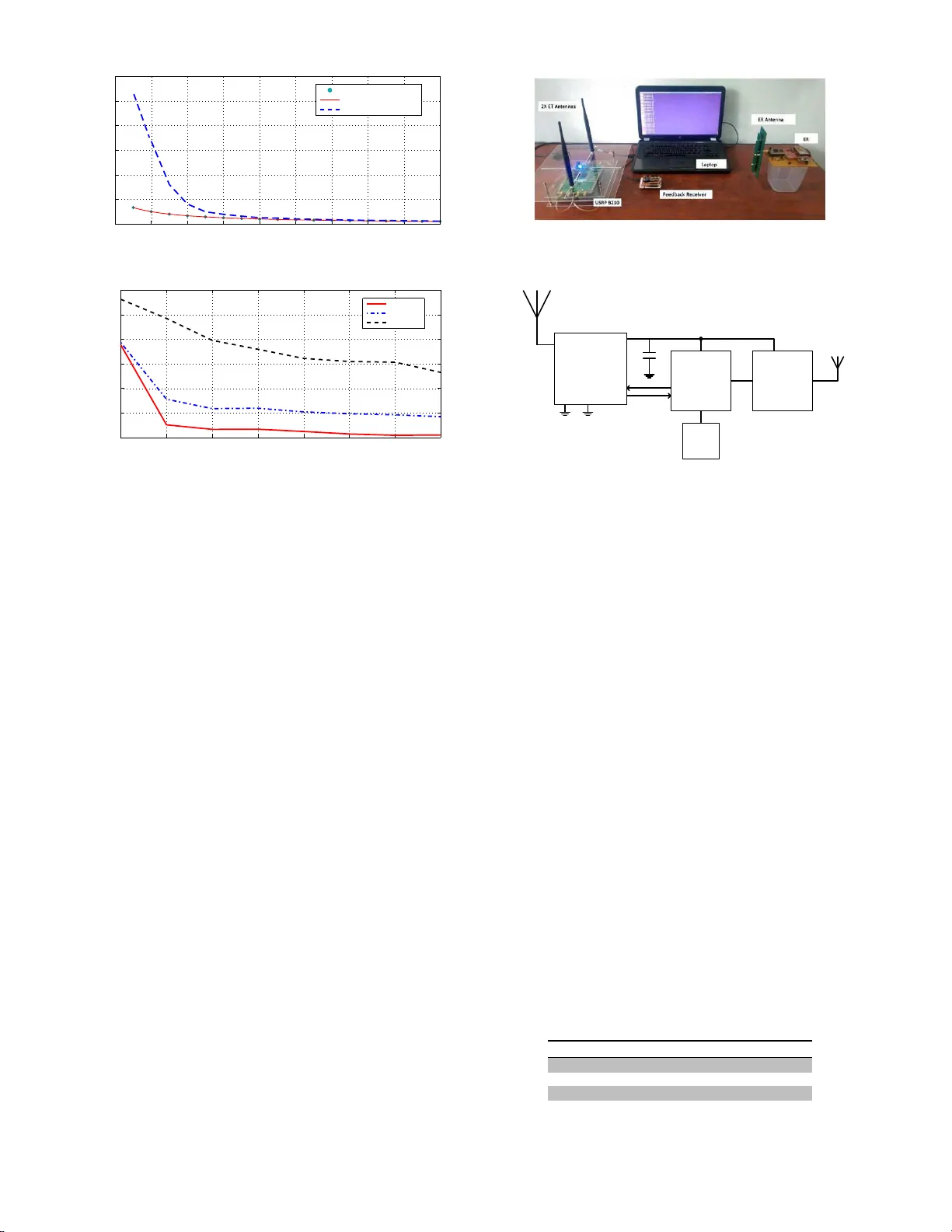
W ireless Ener gy Beamforming using Signal Strength Feedback Samith Abeywickrama Departmen t of Electronic and T elecommunication Engineering, University of Moratuwa, Sri Lanka. Email: samith@ent.mr t.ac.lk Tharaka Samarasinghe Departmen t of Electro n ic an d T elecommunication En gineering , University of Moratu wa, Sri Lan ka. Email: tharak a @ent.mrt.ac.lk Chin Keong Ho Institute for Infoco mm Research , Agency for Science, T ech nology an d Research (A-ST AR), Singap ore Email: hock@i2r .a-star .edu . sg Abstract —Multiple antenna techniques, that allow ener gy beamf orming, hav e been looked upon as a p ossib le candidate fo r increasing the efficiency of the transfer process between the en ergy transmitter (ET) and the energy re ceiver (ER) in wireless en ergy transfer . This paper introduces a n ovel scheme that facilitates ener gy beamfo rmin g by uti l izing Receiv ed Signal Strength Indicator (RSSI) values t o estimate the chann el. Firstly , in the training stage, the ET will transmit sequ entially usin g each beamf orming vector in a codebook, wh i ch is pre-defined using a Cramer -Rao lower bound analysis. The RSSI va l ue corres p onding to each b eamf orming vector is fed b ack to the ET , and these values are used to estimate the channel through a maximum likelihood analysis. The results that are obtained are rema rk ably simple, requires minimal processing, and can be easily implemented. Also, the results are general and hold fo r all well known fading models. The paper also validates th e analytical results numerically , as well as experimentally , and it is shown that the proposed method achieves impressiv e results in wir eless energy transfer . I . I N T RO D U C T I O N W ireless energy transfer (WET) fo cuses on delivering en - ergy to c harge fre e ly located devices, over the air interface, using Electrom a g netic ra diation in the radio freque n cy (RF) bands [2]. When it com es to RF signal enab led WET , incr eas- ing the efficiency of the energy transfe r between the energy transmitter (ET) and the energy receiver (ER) is of paramou nt importan ce. Multiple ante n na tec h niques that also en hance the range between the ET and the ERs have b e en looked up on as a possible solution to add ress this concern [3]. This paper propo ses a novel app roach that incr eases the efficiency of a WET system that utilizes multiple antennas to facilitate the energy tran sfer . T o th is end, multiple antenn as at the E T enab le fo c using the transmitted energy to the ERs via beamfo r ming. However , th e coheren t addition of the signals transm itted fro m th e E T at the ER dep ends on the av ailab ility of chan nel state info rmation (CSI), which necessitates ch annel estimation at the ER in most cases. Th e estimation process inv olves analog to dig ital conv er sion an d baselin e p rocessing which requ ire significant energy [4, 5]. Und er tigh t energy constrain ts and h ardware limitations, such an e stimation proc ess ma y bec ome in feasible at the ER. In th is paper, we propose a mo re energy efficient More comprehensi ve work of this paper is publishe d in IEEE Tran s actions on Signal Processing - [1] method, that allows almo st coheren t addition of the signals transmitted fr om th e ET at th e ER. More over , this is a ch annel learning m ethod that only req uires feedin g back Received Signal Strength Indicator (RSSI) values from the ER to the ET . In most receiv er s, th e RSSI values are in fact already av ailable, and no significant signal pr ocessing is n eeded to o btain them. It should b e noted that the co herent ad dition o f the sign als transmitted from the ET at the ER dep ends directly on the phase of the channels, an d it is interesting that our method focuses on estimatin g the required p hase information by only using magnitud e info r mation a b out the channel. Channel estimation in WET systems normally co n sists o f two stag es. The training stage, wh ere feedback is obtained to estimate the chan nel, and the wireless power beamforming (WPB) stage, where th e actual WET hap pens. Among the existing works that use multiple antennas and sign al strength based ch a n nel estimation, [6] proposes the f ollowing method - ology . In the training stage, firstly , each anten na is individually activ ated, and then , antennas are pairwise activated, in order to ob tain the RSSI values fo r each activ ation. Next, ignorin g the n oise, th ey utilize gathered RSSI values to estimate the channel. In [7], one- bit feed back algorithm [8] is used , a nd in the train ing stage, th e receiver b roadcasts a single b it to the transmitter indicating wh ether the cur rent RSSI is high er or lower than in the pr evious, while the tra nsmitter makes rando m phase perturb ations based on the fe edback of the receiv er . Our proposed schem e is significantly different to [6] and [7 ]. W e focus on a multiple- input-sing le-outpu t (MISO) downlink consisting of two anten nas at the ET and one antenna at the ER. The training stage consists of N time slots. In each of these time slots, the ET will transmit u sing a b eamform ing vector from a pre-d efined codebo ok. Th e E R feeds b ack the analog RSSI value correspon ding to each beamfor ming vecto r , i.e., the ET will rec eiv e N RSSI f eedback values. These N feedback values are utilized to set the beamfo rming vector for the WPB stage. More pr e c isely , fee dback values are utilized to estimate th e phase difference between the two chan nels between the ET and ER, and this difference is cor r ected w h en transmitting in the WPB stage, with the hope of adding the two signals coherently at the ER. Our contr ibutions and the pa per organizatio n can be sum- marized as follows. The system model and the metho dology of obtaining f eedback is explained in Section II. In Sectio n III, we focus on d efining the af orementio ned pre-defin ed cod ebook . T o this en d , we em p loy a Cramer -Rao lower bound (CRLB) analysis, an d define the codebo ok su c h that the estimator of the phase d ifference amon g th e channels achie ves the CRLB, which is the b est perform ance that an unbiased estimator can achieve. In Section IV, we discuss how the feedba ck v a lues can be utilized to set the beamfor m ing vector for the WPB stage, thro ugh a maximu m likelihood analysis. Our analysis takes noise into account unlike [6] , and we p resent the no noise scenario as a spe cial case. The results that we obtain are re m arkably simple, requires min imal pr ocessing, and can be easily implemented at th e ET . Also, the results are g eneral such that th ey will hold for all well known fading models. In Section V, we validate our analytical results numerically . In Section VI, we go on to show that th e prop osed m ethodolo gy can be in fact implemented on hardware. This is not com mon in th e re lated works, an d can be highlighted as another major contribution of this paper . T o this end, we show that, o ur propo sed metho d will ach iev e impressive results giv en how much power can be sav ed at the ER. I t shou ld be also noted that the pro posed methodo lo gy can b e used for any application of beamfor ming wh ere processing capabilities of the receiver are limited. Section VII conclud es the paper . I I . S Y S T E M M O D E L A N D P R O B L E M S E T U P W e consider a MISO channel for WET . An ET consisting of K antenn as d eliv er s energy to an ER c o nsisting of a single anten na, over a wireless med ium. For the clarity of the analysis, and d ue to the direct app lica bility to the experimen tal setup, it is assumed that K = 2 . 1 For this setup, the receiv ed signal at the ER is given by y = h ⊤ x + z , (1) where h =  | h 1 | e j δ 1 | h 2 | e j δ 2  ⊤ is the time-inv ar iant complex random vector having an ar b itrary distribution and repr e sen t- ing the random channel gains b etween the ET an d the ER, x is the 2 -by - 1 vecto r rep resenting the b aseband transmit signal, and z is comp lex ra n dom additive noise. W e assum e a qu a si static block fading ch annel. The baseband transmit signal is defined as x = b s , where s is the tr a n smit symb ol with unit power , and b is the 2 -by- 1 beamformin g vector . For this setup, the harvested en ergy at the ER is given by Q = ξ E  k y k 2  , (2) where ξ denotes the co n version efficiency of the energy har- vester [9], and the expectation is performe d over the random noise. It is n ot hard to see that for a given ξ , the energy transfer is maximized when k y k is maximized, an d this can be a c hieved by an op timal selection of b . In pr a c tice, cha n nel estima tio n is necessary to determine th e op tim al beamfor ming vector b that maximizes th e energy transfer . Howev er, we are particular ly 1 The results in this paper can be easily ex tended to K > 2 scenario by using an approach simila r to the one used in [6 ] for the K > 2 extension. Detail s are skipped due to space limitations. focusing o n applications with tight energy constrain ts at the ER. Thus, such an estimation pr ocess may b ecome infeasible as channel estimation in volves an a log to d igital con version and baseline processing, which require sig nificant energy . Therefo re, we focu s on introd ucing a mo re en ergy efficient method of selecting the beamfor ming vector by only feeding back RSSI values from the ER to the ET . It should b e noted that the feedback is a sin gle analog value, and hence, no significant signal p r ocessing is requ ir ed. In most recei ver circuits, this RSSI value is in fact alread y av ailable. The pr oposed schem e consists of a training stage and a WPB stage. The training stag e c onsists o f N time slots. I n the i th training slot, where i = 1 , . . . , N , the ET uses beamform ing vector b i for wir eless beam forming , and the E R feeds back the analog sign al strength, ba sed on the measured RSSI, for the c orrespon ding transmission. A f ter c ompleting th e trainin g stage, the ET will determ in e th e beamformin g vector q to be used for the WPB stage. Th e ER does not sen d any feed back in this stage, and typically , the WPB stage is lo nger than the training stage to reduce the overhead incu rred in the WPB. W e d efine code book B = [ b 1 . . . b N ] that in c ludes N beamfor ming vectors. Mor eover , b i takes the form of  1 e j θ i  ⊤ , where θ i is the i th element in Θ ( i = 1 , . . . , N ), which is a p redefined set that includes ph ase values between 0 and 2 π . For imp lementation convenience, the cod ebook is predeterm ined and do es not dep end on the sign al streng th feedback , but the WPB vector q is designed based on all the signal strength feedback v alu es. Further , we shall employ estimation theo ry and the conc e pt of th e CRLB in o rder to define B . In the training stage, the pair o f antenn as at the ET is simultaneously activated fo r each e le m ent in B , and the co rrespond ing RSSI value is fed -back throu gh a wireless feedback chann el. T h at is, we have N RSSI values at the ET , and we fo cus on estimating a near optimal b eamform ing vector q based on these RSSI feedb ack values, with a foc u s of comb ining the spatial sign als from the ET coheren tly at the ER. Using (1), and the pro posed meth od o f beamfor m ing, the received signal th at is related to the i th RSSI feedback value can be written as y i = | h 1 | e j δ 1 s + | h 2 | e j δ 2 e j θ i s + z . (3) The cor respond in g i th instantaneou s RSSI value can be ex- pressed as R i =    | h 1 | e j δ 1 s + | h 2 | e j ( δ 2 + θ i ) s    2 + w i =  | h 1 | 2 + | h 2 | 2 +2 | h 1 || h 2 | cos ( θ i − δ 1 + δ 2 )  + w i = α + β cos ( θ i + φ ) + w i , (4) where α = | h 1 | 2 + | h 2 | 2 , β = 2 | h 1 || h 2 | , and φ = δ 2 − δ 1 (the phase dif f erence between h 2 and h 1 ). W e use w i to represent the effect of n oise on R i . Th e noise term w i includes all noise related to the measur ement process, including noise in the channel, circu it, a n tenna matching network and rectifier . Since we are assumin g a block fading model, h can be considered to be unkn own, but n on v ar ying (fixed) du ring the train ing stage an d the subsequen t beamformin g . Ther efore, the r andom n ess in (4) is caused only by the n o ise co m ponen t w i . For tractability , an d without loss of gen erality , we assume w = [ w 1 , . . . , w N ] ⊤ to be an i.i.d . Gaussian ra ndom vector, having zer o mean and v ar iance σ 2 . Also note that the Gaussian distribution lead s to the worst-case CRLB performa nce fo r any estimation problem [10]. From (4), it is easy to show that the RSSI value is maximized (leading to op timal energy tra n sfer in the WPB) when θ i = − φ , i.e. , the optimal beamform in g vector b φ = [1 e − j φ ] ⊤ . Hence, our go al is to estimate the ph ase difference of the two cha n nels, an d we d e note th e estimate using ˆ φ . Also from (4), the RSSI d epends on two more un k nown so-called nuisance parame ters α and β . Hence, the parameter vector is giv en by [ α β φ ] ⊤ . Further , it can be shown that we n e e d at least three RSSI values ( N > 3 ) in order to estimate φ . 2 T o imp lement the p roposed meth od in this paper, we shou ld first define Θ . In the next section, we define Θ by perfo rming a CRLB a n alysis o n the p arameter vector . Then, Θ will b e u sed to d efine the code b ook B . In Section I V, we discuss how the RSSI fe edback values associated to the beamformin g vecto rs in B can be used to estimate φ thro ugh a maximu m likelihood analysis. I I I . C R A M E R - R AO L O W E R B O U N D A N A L Y S I S The CRLB is directly related to the acc uracy of an estima- tion p rocess. More precisely , the CRLB gives a lower bou nd on th e variance of an un biased estimator . T o this e nd, su ppose we wish to estimate th e p arameter vector ϕ = [ α β φ ] ⊤ . The u nbiased estimator of ϕ is deno ted by ˆ ϕ = [ ˆ α ˆ β ˆ φ ] ⊤ , where E { ˆ ϕ } = ϕ . The v aria n ce of the un b iased estimator v ar( ˆ ϕ ) is lower - bound ed by th e CRLB o f ϕ which is denoted by CRLB ϕ , i.e. , v ar ( ˆ ϕ ) > CRLB ϕ . Mo reover , CRLB ϕ is giv en by the in verse of FIM ϕ , which is the Fisher infor mation matrix (FIM) of ϕ . Since no other unb iased estimator of ϕ can ach iev e a v ar ian ce smaller than the CRLB, th e CRLB is the be st perfo rmance that an unbiased estimato r can achie ve. Hence, we select Θ such that the estimator achieves the CRLB, an d hence, the variance is minimized. It shou ld be also noted th at th e Gaussian distrib u tion min imizes/maximizes th e FIM/CRLB [11]. Ther efore, due to the Gaussian assump tion made on th e noise power in (4), we ar e m inimizing the largest or the worst case CRLB. Using (4), th e N -by - 1 vector rep resenting N RSSI ob ser- vations can be written as R = x ϕ + w , (5) where x ϕ is a N -b y - 1 vector of wh ich the i th elem ent takes the for m of α + β cos( θ i + φ ) . Since x ϕ is indepen dent o f w , R in (5) has a multiv a r iate Gau ssian distribution, i.e. , R ∼ N ( x ϕ , C ) , 2 It can be shown that the CRLB is unbounde d if N < 3 rega rdless of the choice of codebook. W e do not provide formal proof details due to space limitat ions. where C = σ 2 I N is the covariance matrix , and I N is the N - by- N identity matrix. W e will specifically focus on φ , which is the main p arameter o f interest, and deri ve the CRLB o f its estimator . Then , we w ill find the set o f values { θ i } N i =1 that will minimize the der i ved CRLB. The CRLB o f φ is fo r mally presented throug h the following lem ma. Lemma 1: The CRLB of parame te r φ is given by CRLB φ = σ 2 N − 1 X i =1 N X j = i +1 h cos( θ i + φ ) − cos( θ j + φ ) i 2 β 2 N − 2 X i =1 N − 1 X j = i +1 N X k = j +1 ∆ i,j,k , where ∆ i,j,k = h sin( θ i − θ j ) + sin( θ j − θ k ) + sin( θ k − θ i ) i 2 . W e will only p r ovide a sketch of the proof due to space limitations. Th e i th row of ∂ x ϕ ∂ ϕ is given by [1 cos( θ i + φ ) − β s in( θ i + φ )] , for i = 1 , . . . , N . By using the FIM of a Gau ssian rand om vector in [1 2], and using the fact that C is indep e ndent of ϕ , th e FIM of R ca n be written as FIM ϕ ( R ) = h ∂ x ϕ ∂ ϕ i ⊤ C h ∂ x ϕ ∂ ϕ i . The CRLB of the i th element in ϕ can be obtained by the i th diagon al element of the inv er se FIM . Theref ore, compu tin g the third diagon al element of the in verse of FIM ϕ ( R ) completes the proof . Since we want to find { θ i } N i =1 that will m inimize the derived CRLB for any given φ , we a vera g e out the effect of φ by considerin g the expec tation over φ . T o this end, we assume φ to be uniform ly d istributed in (0 , 2 π ] . This lead s to the modified Cramer - R ao lower bo und (MCRLB) [13], an d it is formally presen ted throu g h th e following lemma. The proo f is skipped since its trivial. Lemma 2: The MCRLB of param eter φ is gi ven by MCRLB φ = E φ [CRLB φ ] = σ 2 N − 1 X i =1 N X j = i +1 h 1 − cos( θ i − θ j ) i β 2 N − 2 X i =1 N − 1 X j = i +1 N X k = j +1 ∆ i,j,k . (6) Determining the { θ i } N i =1 analytically for a general case is not straightfor ward due to the c omplexity o f (6). There f ore, we will first focu s on the N = 3 ca se, an d derive { θ 1 , θ 2 , θ 3 } that m inimizes the M CRLB. T o this e nd, without any loss of generality , we assume θ 1 to be zer o and θ 2 and θ 3 are set relative to θ 1 . Then, we repeat the process for N = 4 . From these two deriv ations, we can observe a pattern in the MCRLB φ minimizing θ i values, and we define Θ by making u se of this pattern . I n Section V, th rough num erical ev aluation s, we validate the selection of Θ f or arbitrar y values of N . Lemma 3: Let θ 1 = 0 . If N = 3 , MCRLB φ is minimized when Θ = { 0 , 2 π / 3 , 4 π / 3 } , and the corr e sp onding m inimum MCRLB φ is g i ven by 2 σ 2 3 β 2 . If N = 4 , MCRLB φ is m in imized when Θ = { 0 , π / 2 , π, 3 π/ 2 } , and the correspon ding minimum value o f MCRLB φ is giv en by 2 σ 2 4 β 2 . Pr oof: By d ifferentiating (6) with respect to θ 2 and θ 3 , respectively , and by setting θ 1 = 0 , we ob tain two equations consisting o f θ 2 and θ 3 . E quating th e two equatio ns to zero and simultaneously so lving them u nder the co nstraints θ 2 , θ 3 ∈ (0 , 2 π ] and θ 1 6 = θ 2 6 = θ 3 giv es us θ 2 = 2 π / 3 and θ 3 = 4 π / 3 . Evaluating the Hessian matrix at the stationary point (0 , 2 π / 3 , 4 π / 3) shows that the stationary po int is a minimu m. Substituting (0 , 2 π/ 3 , 4 π / 3) in (6) gives us 2 σ 2 / 3 β 2 , which completes the pro of for N = 3 . Following the same lines fo r the N = 4 case comp letes the p roof of the lemma. It is interesting to no te th a t in both cases, the p hase v alue s in Θ are equally spaced over [0 2 π ) . For an examp le, when N = 3 , | θ 1 − θ 2 | = | θ 2 − θ 3 | = | θ 3 − θ 1 | = 2 π / 3 . When N = 4 , the phase d ifference be tween adjacent elements in th e set turn s out to be 2 π / 4 . Also, by o bserving this pattern,we can exp e c t the minimum MCRLB φ for arbitr ary N to take the fo rm of 2 σ 2 N β 2 . T o this end, we will d efine Θ for N elements as follows. Definition 1: Θ is a set of phase values between 0 and 2 π , and it is defin e d to b e Θ = { θ 1 , . . . , θ N } , where θ i = 2( i − 1) π N for i ∈ { 1 , . . . , N } . The intuition behind this de fin ition is that getting RSSI values with the maximu m spatial diversity p rovides us the best estimate. Using th e phase values in Θ , N RSSI feed back values can be o btained. The n ext q uestion is how these N feedback values can be used to estimate the phase difference between the two channels. T h is, qu e stio n is a d dressed in the next section. I V . E S T I M A T I O N O F C H A N N E L P H A S E D I FF E R E N C E φ W e will first look at a simplified scena rio similar to [ 6] by assuming that there is no noise. If there is no noise, we hav e R i = α + β cos ( θ i + φ ) , and we can consider N = 3 and simply calcu late φ by so lv ing three simu ltaneous equatio ns. The resu lt is formally p r esented in the following theo rem an d this value of φ sho uld intu itiv ely give satisfactory resu lts in low n oise en viro nments. The pro of is skipped as it is trivial. Theor em 1: I n a noiseless environment, th e ph ase difference between the two channels is giv en by ˆ φ = tan − 1 λ 1 , 3 sin  θ 1 + θ 2 2  − λ 1 , 2 sin  θ 1 + θ 3 2  λ 1 , 2 cos  θ 1 + θ 3 2  − λ 1 , 3 cos  θ 1 + θ 2 2  ! (7) where λ i,j = R i − R j and i, j ∈ { 1,2,3 } . It should be no ted that φ has an ambigu ity du e to the use of ta n − 1 , an d φ can be either φ or φ − π . The easiest way to resolve this ambiguity is b y ascertaining two furth er RSSI feedb ack values from the ER for the two beamfor ming vectors [1 e − j φ ] ⊤ and [1 e − j ( φ − π ) ] ⊤ and picking the o ne that provides the better energy transfer . Also note that [6] uses a similar approac h , but it req uires four more feedback v alues to resolve the ambig uity as the phase difference is given as a cosine in verse. Now , we will focus on a scen ario with noise. Based on th e assumption that the noise power is i.i.d. Gaussian, estimating φ becomes a classical pa rameter estima tio n problem. A m a x- imum likelihood estimate of φ can be ob tained by findin g the value o f φ that minimizes E , N X i =1 h R i − ( α + β cos ( θ i + φ )) i 2 . Differentiating E with re sp ect to φ , and setting it equal to z e ro giv es us N X i =1 R i sin ( θ i + φ ) = α N X i =1 sin ( θ i + φ )+ β 2 N X i =1 sin [2( θ i + φ )] . (8) It is not h a rd to see that to estimate φ , we hav e to first estimate α and β . These no n -essential parame ters are refer red to as nuisance p a rameters [ 14]. Howe ver, due to the way we have d efined Θ , it is intere stin g to see th a t we can obtain an ML estimate of φ withou t estimating the nuisance par ameters. These ideas are formally presented in the following theo rem. Theor em 2 : For a sample of N i.i.d . RSSI observations, φ can be estimated by ˆ φ = ta n − 1       − N X i =1 R i sin θ i N X i =1 R i cos θ i       , (9) where θ i = 2( i − 1) π N . Pr oof: When θ i = 2( i − 1) π /N , using series o f trigon o- metric fun ctions in [15], we have P N i =1 sin( θ i + φ ) = P N i =1 sin [2( θ i + φ )] = 0 . Th erefore, (8) can be simplified and written as P N i =1 R i sin ( θ i + φ ) = 0 , which is indepen dent o f α and β . Expand ing sin ( θ i + φ ) allows us to obtain (9), which completes the proof . Here, φ ag ain has an ambiguity due to the use of tan − 1 , and it can also be resolved by ascertainin g two m o re f eedback values. No te th at the result in Theorem 2 is easy to calcu late, requires minimal pr ocessing, and can b e easily implemen ted at the ET . Also, the result ho ld s for a ll well kn own fading models. W e should stress that this rather simple expression was possible due to the CRLB analysis perform ed in Section III to defin e Θ . In the next section , we will validate our re su lts using numerica l evaluations. V . N U M E R I C A L E V A L U A T I O N S In L emma 3, we have focused on MCRLB φ , and we have given th e fo r mal proof for th e minimum MCRLB φ , considerin g N = 3 and N = 4 , respe c tively . Then, based on the pattern , we expected that the minimum MCRLB φ = 2 σ 2 N β 2 for arbitrary values of N . Fig. 1 validates this result for arbitrary values of N . For the nu merical ev aluatio n , we have set β = σ = 1 , and we have calculated MCRLB φ accordin g to Lemma 2, while setting the ph ase values accordin g to Θ in Definitio n 1. W e can see that setting the ph a se values accordin g to Definition 1 a llows us to achieve the m inimum MCRLB as the values lie on the 2 /N curve. The figur e also 2 4 6 8 10 12 14 16 18 20 0 1 2 3 4 5 6 N - No of f ee dbac k values MC RLB φ Θ according to Definition 1 2/N curve Ramdomly generated Θ Fig. 1. The behavior of the M CRLB φ with N when β = σ = 1 . 3 4 5 6 7 8 9 10 0 2 4 6 8 10 12 N - No o f fee dback v alues Me a n Absolut e Err or (Degrees) SNR=40dB SNR=20dB SNR=10dB Fig. 2. The behavio r of the Mean Absolute Error (MAE) of ˆ φ for three dif ferent SNR val ues when β = σ = 1 . shows how the a verag e MCRLB φ behaves when the phase values in Θ are cho sen random ly , f or a gi ven N . The av erage MCRLB φ values always lie ab ove th e 2 / N cur ve. Also, it can be seen th at a MCRLB φ value obtained by a ran d omly generated Θ can be achieved b y lower num ber of feedback values when Θ is de fin ed acco rding to Definitio n 1. Th is is vital as we are dealing with a receiver with a tight energy constraint. Also, as expected , we can observe that when N increases, the lower b ound on the variance of ˆ φ decreases. In Theo r em 2, we have presen te d an ML estimate of φ . Fig. 2 illustrates the behavior of the ph ase e stimation er ror with N for d ifferent SNR values. Θ is defin ed accord ing to De finition 1. F o r the higher SNR values, erro r conv erges to zero rap idly than the lower SNR values. It is interesting to note that even when N = 3 , the phase error is no t significantly large. Next, we will further validate o ur results experimentally . V I . E X P E R I M E N TA L V A L I D A T I O N The implementatio n of ou r ER is shown in Fig. 4. W e use Powercast P111 0 power - harvester , which has an operating band ranging fro m 90 2 to 928MHz. P1110 has an analog output ( D OUT ), which provide s an analog voltage lev el co r- respond in g to the RSSI. As the storag e de v ice of our design, we use a lo w leakage 0. 22F super-capacitor . Th e output of P1110 charges the super-capacitor and the super-capacitor powers the micr ocontro ller , the feed b ack transmitter an d the sensors. An Ultra-Low-Po wer MSP430F55 29 microcontro ller is used to read the RSSI v alu es and transmit them v ia the feedback tr ansmitter . When functionin g, the micr ocontro ller and the feedback transmitter ar e on sleep mode , an d after each 500 ms interval, both wake up from sleep in order to read the RSSI and transmit it to the ET . NORDIC nRF24L01 Fig. 3. Experi m ental setup P1110 Microcontroller GND Sensors Feedback D ALK OUT D RF V SET IN OUT Power Receiving Antenna Antenna Super-capacitor MSP430F5529 Transmitter nRF24L01 Fig. 4. The hardware block diagram of E R. single ch ip 2.4GHz transceiver has been used as f eedback transmitter . When the ER op erates in th e activ e mod e (read ing RSSI values and transmitting), it consumes on ly 12.8 µ J/ms and it consumes n egligible energy in sleep mode. The SDR used in our ET is USRP B21 0, which has 2 × 2 MIMO capability . CR YSTEC RF power amplifiers (CRB AMP 100- 6000) are used to amp lify the RF power o utput of the USRP B210. All the r eal-time signal processing task s, chann el phase difference ( φ ) estimation and setting beamfo rming vectors in both trainin g and WPB stag es were p e r formed on a laptop using the GNU Rad io fr amew o rk. W e use 9 1 5Mhz as the beamfor ming frequen cy . The same tran sceiv er chip used in the ER, nRF24L01, is used as the feedb ack receiver at the ET side. For th e experiment, the ET and the ER are 2 meters apart. Using this setup, for N = 3 , Fig. 5 illustrates th e train in g stage and the WPB stage, including ambiguity resolving, and we can see a clear gain by the proposed method . Then, we focused on validating the r esult on phase esti- mation. For this, we changed θ i from 0 to 360 degrees with 1 ◦ resolution, and collected all re spectiv e RSSI values (see Fig. 6). Since it was not practical to collect all the 360 RSSI values using the harvested energy via the f eedback transmitter, we used a wired feedback for this experiment. Fig. 6 shows T ABLE I E X P E R I M E N TA L RE S U LT S N ˆ θ Error | ˆ θ − 79 ◦ | 3 71 ◦ 8 ◦ 4 77 ◦ 2 ◦ 5 78 ◦ 1 ◦ 6 76 ◦ 3 ◦ 0 1 2 3 4 5 0 50 100 150 200 250 300 350 Fe e d bac k n o. RSSI (mV) T raining stage Resolving ambiguity WPB stage WP B Fig. 5. The RSSI v alues corresponding to each stage when ET and ER are 2 m eters apart and N = 3 . 0 50 100 150 200 250 300 350 0 20 40 60 80 100 120 140 160 180 200 θ (Deg rees ) RSSI (m V) RSSI Maximum RSSI RSSI in WPB, N=3 RSSI in WPB, N=4 RSSI in WPB, N=5 79 i Fig. 6. The RSSI value s when θ i is chang ed from 0 ◦ to 360 ◦ with 1 ◦ resoluti on. that the m aximum RSSI occurs when θ i = 79 ◦ . Therefor e, the maximu m energy transfer hap pens at that point. Using the same set of values, we estimated ˆ φ ( Θ de fin ed accord ing to Definition 1) for N = 3 , N = 4 , N = 5 an d N = 6 , respectively . The results are tabulated in T able I. It is not hard to see th at th e e r rors ar e significantly small, a n d they are consistent with the nu merical e valuations as well. Furthe r, by using our prop osed scheme, an d based on th e assumption that the conversion efficiency of the power - harvester is fixed, w e can extend the range of the ER b y 52% on a verage. This has been calc u lated based o n the experimental r esults co n sidering free space loss. V I I . C O N C L U S I O N S This pa p er has propo sed a n ew channel estimation approa ch to be used in a mu ltiple antenna WET system. The ET will transmit using beamformin g vecto r s fro m a codebook , which has b een pr e-defined u sin g a Cramer-Rao lower bo und analysis. RSSI value correspo nding to eac h beamf orming vector is fed back to the ET , and these values h av e been utilized to estimate the cha n nel throug h a m aximum likelihood analysis. T he results th a t have been obtained ar e simple, requires min imal processing, and ca n be e asily implem ented. The p aper has also validated the analytical resu lts numer ically , as well as experim entally . I t has been shown tha t th e results in the paper are more appealing as com pared to existing channel estimation methods in WET , e specially when there is tight energy constrain ts and h a rdware limitations at the ER. It is also im portant to po int ou t th a t alth o ugh ch annel estimation for multiple antenna WET systems has been considered in this paper, the proposed methodolog y can be used for any application o f beamfo rming where pr ocessing capabilities of the receiver are limited. Furthe r an alytical and experim ental results related to the p roposed metho dology will be presented in future work. R E F E R E N C E S [1] S. Abeywickram a, T . Samara singhe, C. K. Ho, and C. Y uen, “Wi reless energy beamf orming using received signal strength in dicator feedback , ” IEEE T rans. Sig nal Pr ocess. , vol. 66, p p. 224–2 35, Jan. 20 18. [2] R. Zhang an d C. K. Ho, “MIM O broa d casting for simul- taneous wireless info rmation and power transfer, ” IEE E T r a ns. W ir eless Co m mu n. , vol. 1 2 , pp . 198 9 – 2 001, M ay 2013. [3] X. Chen, Z. Zhang , H. H. Chen, and H . Zhang, “En- hancing W ir eless In formatio n and Power T ransf e r by Exploiting Multi-Antenn a T echniq u es, ” IEEE Commu n. Mag. , vol. 53, pp. 133–14 1, Apr . 201 5. [4] A. Huhn and H. Sch wetlick, “Channel estimation meth- ods for div er sity and MIMO in LR-WP AN systems, ” in Pr oc. IEEE Intern a tional Confer ence on Consu mer Electr onics , pp. 223 – 224, Jan. 201 0. [5] Q. W an g, D. W u , J. E ilert, and D. Liu, “Cost ana ly sis of chan nel estimation in MIMO-OFDM fo r software defined radio, ” in P r oc. I EEE W ir eless Communications and Networking Confer en ce , p p. 935 – 939, Apr . 2008. [6] S. Lak shmanan, K. Su ndaresan, S. Ran g arajan, a n d R. Si vakumar, “Practical beamf orming based on RSSI measuremen ts using o ff-the-shelf wire less clients, ” in Pr oc. Internet measurement confer e n ce , p p. 410–4 16, Nov . 200 9. [7] F . Quitin, M. U. Rahman, R. Mud u mbai, and R. Mu dum- bai, “Distributed beamforming with so ftware-defined ra- dios: Frequency synch ronization an d digital feedba ck, ” in Pr oc. IEEE Globa l T eleco mmunicatio ns Con fer ence , pp. 4787 – 4792, Dec. 2012. [8] J. Xu and R. Zhang, “E nergy beamform ing with one- bit fee dback, ” IEEE T r an s. Sign al Pr ocess. , vol. 62, pp. 5370–5 381, Oct. 20 14. [9] S. Bi, C. K. Ho, an d R. Zh ang, “Recen t advances in joint wireless en ergy and info rmation transfer, ” in Pr oc. IEEE Information Theory W orkshop , pp. 341 – 34 5, Nov . 201 4. [10] P . Stoica and P . Babu, “The G a ussian data assumption leads to the largest Cramer-Rao boun d , ” IEE E Signa l Pr ocess. Mag. , vol. 28, pp. 132 – 133, May 201 1. [11] S. Park, E. Serped in, and K. Qaraqe, “Gaussian assump - tion: Th e least fa vorable but the mo st useful, ” IEE E Signal Pr o cess. Mag. , vol. 30, pp. 183 – 18 6, Ap r . 201 3. [12] S. Kay , Fu ndamen tals of S tatistical Signa l P r ocessing: Estimation Theory . Prentice- Ha ll, 19 93. [13] T . Pany , N a vigation S ig nal Pr o cessing for GNSS S oftwar e Receivers . Ar tech House, 1 ed., 2010 . [14] J. C. Spall and D. C. Chin, “On system identification with n uisance p arameters, ” in Pr oc. America n Contr ol Confer en ce , p p. 530 – 531, Jul. 1994. [15] I. Gradshteyn a nd I. Ryzhik, T a ble of Integr als, Series, and Pr oducts Seventh Edition . Academic Press, 2007.