Noise Level Estimation for Overcomplete Dictionary Learning Based on Tight Asymptotic Bounds

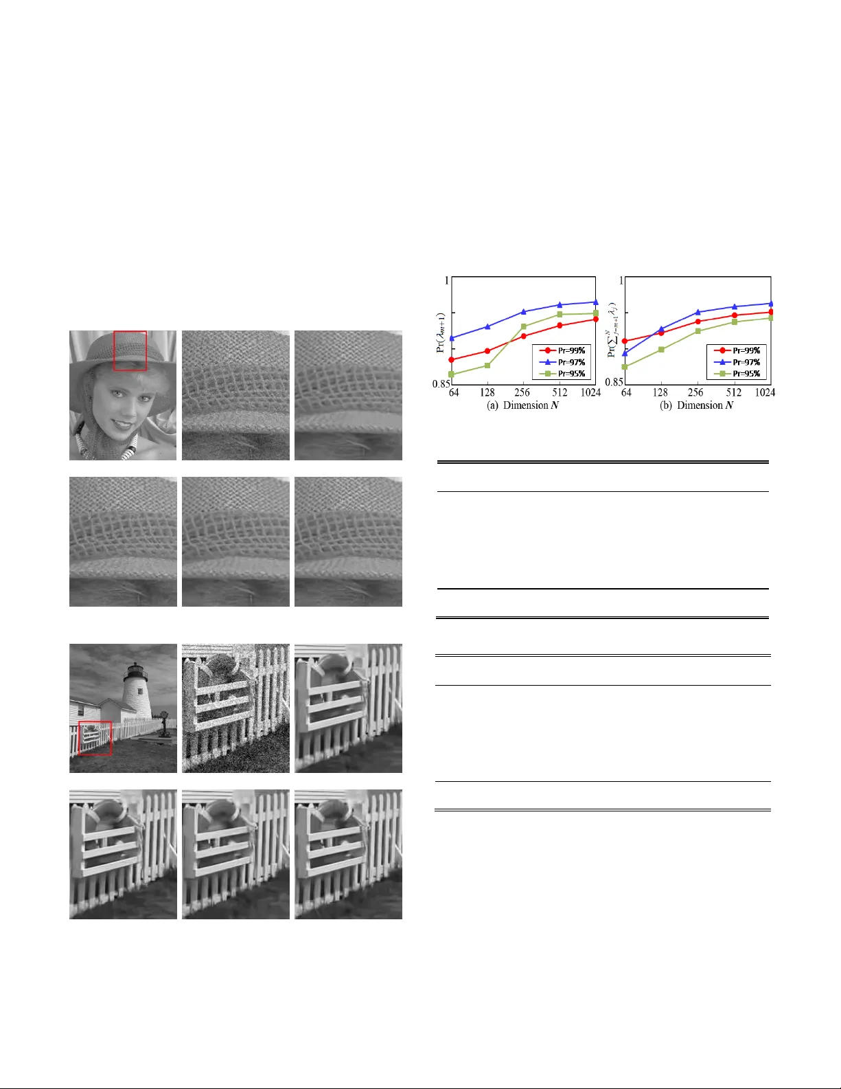
> REPLACE THIS LINE WITH YOUR PAPER IDENTIFICAT ION NUMBER (DOUBLE-CLICK HERE T O EDIT) < 1  Abstract — In this letter, w e address the problem of estimating Gaussian noise level from the trained dictionaries in update stage. We first provide rigorous statistical analysis on the eigenvalue distributions of a sample covariance matrix. Then w e propose an interval-bounded estimato r for noise variance in high dimensional setting. To this end, an effective estimation method for noise level is devised based on the boundness and asymptotic behavior of noise eigenvalue spectrum. The estimation performance of our method has been guaranteed both theoretically and empirically. The analysis and experiment results have demonstrate d that the proposed algorithm can reliably infer true noise levels, and outperforms the relevant existing methods. Index Terms — Dictionary learning, sample covariance matrix , random matrix theory, noise level estimation. I. I NTRODUCTION HE dictionary learning is a matrix factorization problem that amounts to finding the linear com bination of a given signal NM   Y  with only a few atoms selected from columns of the dictionary NK    D  In an overcomplete setti ng, the dictionary matrix D has more columns than rows , KN  and the correspond ing coefficient matrix KM   X  is assumed to be sparse. For most pr actical tasks in the presence of noise, we consider a c ontamination form of the measurement signal ,  Y D X w where the elements of noise w are independent realizations from the Gaussian distrib ution 2 (0 , ) n  N . The basic dictionary learning problem i s formulated as: 2 0 , m in . . F i s t L i   DX Y DX x (1) Therein, L is the maximal number of non-zero elements in the coefficient vector i x . Starting with an initial dictionary, this minimization task can be sol ved by the popular alternating approaches such as the method of optimal directions (MOD) [1] and K -SVD [2]. The dictiona ry trai ning on noisy samples can incorporate the denoising together i nto one it erative process . In general, the residual errors of learning process are determined Manuscript received December XX, 2017; revised XX, 2017; accepted XX, 2017. Date of publication XX, 2017; date of current version XX, 2017. This work was supported by Beijing major scien ce and tech nology projects under Grant Z171100000117008. The associate editor coordinating the review of this manuscript and approving it for publication was Prof. XXXX. R. chen is wi th th e School of Microelectronics, Tianjin University, Tianjin 300072, China (e-mail: rchen@jdl.ac.cn). C. Yang * (Corres ponding author), H. Jia and X. Xie are with National Engineering Laboratory f or Video Technology, Peking University, Beijing 100871, China (e -mail: {csyang, hzji a, donxie}@pku.edu.cn ). Color v ersions of one or more of the figures in this paper are available online at http://ieeexplore.ieee.org. Digital Object Identifier 10 .1109/LSP.2015.2448732 by noise level s [3]. Noise incursion in a trained dictionary can affect t he stability and accuracy of sparse representation [4]. So the performance of dictionary learning highly depends on the estimation accuracy of unknown noise level 2 n  when the noise characteristics of trained dictiona ries are unavailable. The mai n challenge of estimat ing the noise level lies in effectively distinguishing the signal from noise by exploiting sufficient prior information. The most existing methods have been developed to estimate the noise level from image sign als based on specif ic image cha racteristics [5 ]-[8]. Generally, these works assume that a sufficient amount of homogeneous areas or self-similarity patches are contained in natural images . Thus empirical observations, singul ar value decomposition (SVD) or statistical properties can be applied on carefully selected patches. However, it is not suitable for estimating the noise level in dictionary update stage because only few atom s for sparse representation cannot guarantee the usual assumptions. To enable wide r applications and le ss assumptions, more recent methods estimate the noise le vel based on principal c omponent analysis (PCA) [9 ], [10]. These methods underestimat e the noise level since they only take the smallest eigenvalue of block covariance matrix. Although later work [ 11 ] has m ade efforts to tackle these problems by spanning low dimensional subspace, the op timal estimation for true noise variance is still not achieved due to the inaccuracy of subspace segmentation . As for estimating the noise variance techni ques , the scaled m edian absolute deviation of wavel et coefficients has been widely adopted [12]. Leveraging the results from random matrix theory (RMT), the median of sample eigenvalues is also used as an estimator of noise variance [13]. However, these estimators are no longer consiste nt and unbiased when the dictionary matrix has high dim ensional structure. To solve the aforementioned problems, we propose to accurately estim ate noise va riance by using exact eigenvalues of sample covariance matrix. A ti ght asymptotic bound for extreme eigenvalue s is constructed to separate the subspaces between the signal and noise. For traine d dicti onaries with low-sample sizes and high dimensions, a bounded estimator provide s a consistent inference on noise vari ance. The practical usefulness of our method is num erically illustrated. II. T IGHT B OUND FOR N OISE E IGENVALUE D ISTRIBUTION In this section, we analyze the asymptotic al distribution of the ratio of extreme eigenvalues of a sample covariance matrix based on the limiting RTM la w. Then a tight bound is derive d. Noise Level Estimation for Overcomplete Dictionary Learning Based on T ight Asymptotic Bounds Rui Chen , Member, IEEE, Changshui Yang, Huizhu Jia and Xiaodong Xie T > REPLACE THIS LINE WITH YOUR PAPER IDENTIFICAT ION NUMBER (DOUBLE-CLICK HERE T O EDIT) < 2 A. Eigenvalue Subspaces of Sample C ovariance Matrix We consider the sparse approxim ation of each observed sample N i  y  with s prototype atoms selected from learned dictionary D . With respect to the sparse model (1) , we ai m at estimating the noise level 2 n  for an elementary trained dictionary s D containing a subse t of t he atom s 1 {} i s i  d . At each iterative step, the noise level 2 n  goes gradually to zero when updating towards the true dictionary [14]. The known noise variance is helpful to avoid noise incursio n and determine the sample size, the sp arsity degree and even the performance of the true underlying dictionary [15]. To deri ve the relationship between the eigenvalues and noise level, we first construct th e sample covariance m atrix of dictionary s D as follows: T 11 1 1 ( )( ) , 1 S ii ss i i i s s        d d d d d d (2 ) According to (2), the square matrix s  has N dimensions with the sparse condition N s  . Based on the symmetric property, this matrix is decomposed into the product of three matrices: an orthogonal matrix U , a diagonal matrix and a transpose matrix T U , which can be selected by satisfying T  U U I . Here, this transform process is writt en as: T 11 ( ,..., , , ..., ) S m m N       U U = di ag (3) Given 12 ... N       , we exploit the eigenvalue subspaces to enable t he se paration of at oms from no ise. To be m ore specific, we divide the e igenvalues into two sets 12  S S S  by finding the appropriate bound in a spiked population model [16]. M ost structures of an atom lie in low-dimension subspace and thus the le ading eigenvalues in set   1 1 m i i    S are m ainly contributed by atom it self . The re dundant-dimension subspace   2 1 N i im    S is dominated by the noise. Because the atom s contribute very little to this la ter portio n, we take all the eige nvalues of 2 S into consideration to estimate the noise variance while elim inating the influence of trained at oms. Moreover, the random variables   1 N i im   can be considered as the eigenvalues of pure noise covariance matrix  w , wh ose dim ensions are N . B. Asymptotic Bound for Noise Eigenv alues Suppose the sample matrix  w has the form T ( 1 ) s    w HH , where the sample entries of H are independently generated from the distribution 2 (0 , ) n  N . Then the real matrix T  M HH follows a standard Wishart distribution [17 ]. The ordered eigenvalues of M are denoted by m ax m in ( ) ( )       MM . In the high dimensional situation:   0, / N s    as s fixed and N  , the T racy-Widom law gives the limiting distribu tion of the largest eigenvalue of the large random matrix M [18]. Then we have the following asym ptotic expression: 2 TW1 ma x Pr ( ) n z F z          (4) where TW1 () Fz indicates the cumulative distribution function with respect to the Tracy-Widom random variable. In order to improve both t he approximation accuracy and convergence rate, even only with few atom samples, we need choose the suitable centering and s caling param eters ,   [ 19 ]. By the com parison between different values, such param eters are defined as     13 2 1 / 2 1 / 2 1 / 2 1 / 2 1 / 2 1 / 2 11 N N N s s s                      (5) The empirical distribution of the eigenvalues of the large sample matrix converges almost s urely to the Marcenko-Pastur distribution on a finite support [20]. Based on the generalized result in [21], when N  and   0,    , with probability one, we derive limit ing value of the smallest eigenvalue as   2 2 m in 1 n     (6) According to the asymptotic distributions described in the theorems (4) and (6), we further quantify the distribution of the ratio of the maximum eigenvalue to minimum eigenvalue in order to detect the noise eigenvalues. Let 1 T be a detection threshold. Then we find 1 T by the following expression:       2 1 1 1 2 2 2 22 2 11 TW1 max max max min min max 1 11 Pr Pr Pr Pr n n n n T T T N TT NN F s ss                                                            (7) Note that there is no closed-form expression for the function TW 1 F . Fortunately, the values of TW 1 F and the inverse TW1 1 F  can be numerically computed at certain percentile points [16]. For a required detection probability 1  , this leads to   TW 1 2 1 1 1 1 () N T s F        (8) Plugging the definitions of  and  into the Eq. (8), we finally obtain the threshol d           TW 1 2 23 1 1 2 1 1 6 1 6 1 2 1 2 1 2 1 2 1 2 1 2 ( ) 1 N N T F N N s s s s s                 (9) When the detection thresho ld 1 T is known in the given probability, it means that an asym ptotic upper bound can also be obtained for determining the noise eigenvalues of the m atrix  w because the equality m ax m in 1 N m     holds. In general, the noise eige nvalues in the set 2 S surround the true noise variance as it follows the Gaussian distribution. The estimated largest eigenvalue 1 m   should be no less than 2 n  . The known smallest eigenvalue N  is no more than 2 n  by the theoretical analysis [ 11 ]. The locatio n and value of 1 m   in S are obtained by checking the bound 1 1 N m T     with high probability 1  . In addition, 1  cannot be selected as noise eige nvalue 1 m   . > REPLACE THIS LINE WITH YOUR PAPER IDENTIFICAT ION NUMBER (DOUBLE-CLICK HERE T O EDIT) < 3 III. N OISE V ARIANCE E STIMATION A LGORITHM A. Bounded Estimator for Noise Variance Without requiring the knowledge of signal, t he threshold 1 T can provide good detection performance for finite , N s even when the ratio / N s is not too large. Based on this result, more accurate estimation ca n be obtained by a veraging all elements in 2 S . Hence, the maximum likelihood estimator of 2 n  is 2 1 1 ˆ N nj jm Nm      ( 10 ) In the low dimensional setting where N is relatively small compared with s , the estimator 2 ˆ n  is consistent and un biased as s  . It follows asymptotically normal distribution as   4 2 22 2 2 (0, ˆ ), n nn Nm s tt       N ( 11 ) When N is large with respect to the sample size s , the sample covariance matrix shows significant deviations from the underlying population covariance matrix. In this context, the estimator 2 ˆ n  might have a negative bias, which leads to overestimation of true noise variance [ 22 ], [ 23 ]. We investiga te the distribution of another eigenvalue ratio. Namely, the ratio of the maximum eigenvalue to t he trace of the eigenvalues is 11 1 () () 1 tr( ) 1 mm N j jm Nm Nm U            w ( 12 ) According to the result in (4), the ratio U also fo llows a Tracy-Widom distribution as both , Ns  . The denom inator in the definition of U is distributed as an independent 2 2 N n N  random variable, and thus has 22 E( ) ˆ nn   and 24 V ar( ) 2 ( ) ˆ nn N s   . It is easy to show that replacing 2 n  by 2 ˆ n  results in the same limiting distribution in ( 4). Then we have 2 1 TW1 ˆ Pr ( ) mn z F z           ( 13 ) Unfortunately, the asymptotic approximation present in (13) is inaccurate for small and even moderate values of N [24]. This approximation is not a proper distribution function. The simulation observations imply that the major factor contributing to the poor approximation is the asymptotic error caused by the constant  [24]. Therefore, a more accurate estimate for the standard deviation of 2 1 ˆ mn   will provide a significant improvem ent. For finite samples, we have 2 4 4 1 1 22 E , E m m n n                   ( 14 ) Using these asymptotic result s, we get the corrected deviation 22 2 () 2 Ns N s N s          ( 15 ) Note that this formula in (15) has corrected the overestimation in the high dimensional settin g. Thus the better approximation for the probabiliti es of the ratio is 2 1 TW1 ˆ Pr 1 ( ) mn z F z              ( 16 ) The determinati on of the distribution for the ratio U is devoted to the correction of the variance estimator. In order to complete the detection of the large deviations of the initial estimator 2 ˆ n  , we provide a procedure to set the threshold 2 T . Based on the result in (16), an approxim ate expression for the overestimation probabili ty is given by 22 1 2 2 2 TW1 1 ˆ ˆ 11 Pr = Pr 1 ( ) n m n m TT TF                               (17) Hence, for a desired probability level 2  , the above equation can be numerically inverte d to find the decision threshold. After some sim plified manipulations, we obtain TW 1 2 1 2 1 = ( 1 )+ T F       ( 18 ) Asymptotically, t he spike eigenvalue 1 m   converges to the right edge of the support 2 ( 1 ) n Ns   as , N s go to infinity. According to the expression in (18), this function turns out to have a simple approximation 2 1 T   in the high probability case. Then the upper boun d 2 1 m T    for the known 2 ˆ n  yields a bias estimation. Finally, the fo llowing expectation holds true : 21 22 ˆ E 1 m nn T Ns           ( 19 ) By analyzing the statistical result in ( 19), t he correction for 2 1 m T    can be approximated as the better estimator than 2 ˆ n  because this bias-corrected estimator is closer to the true variance under the high dimensional conditions. If 2 ˆ n  can satisfy the requirem ent of no excess of the bound 2 1 m T    , the sample eigenvalues are consistent estim ates of their population counterparts. Hence, the opti mal estimator is given by 21 22 ˆ ˆ m in , 1 m n T Ns             ( 20 ) B. Implementation Based on the construction of two thresholds, we propose the noise estimation m ethod for dictionary learning as follows: Step 1. Compute the eigenvalues   1 N i i   of the sample covariance matrix S  , and order 12 ... N       . Step 2. Set the probability l evels 1  and 2  . Step 3. Compute two thresholds 1 T and 2 T . Step 4. Obtain the location 1 m  of noise eigenvalues and the value of 1 m   by checking whether 1 1 N m T     is true. Step 5. Compute the initial estim ator 2 ˆ n  . Step 6. Compare two estimators in (20) and select the minimum as the optim al estimation of 2 n  . > REPLACE THIS LINE WITH YOUR PAPER IDENTIFICAT ION NUMBER (DOUBLE-CLICK HERE T O EDIT) < 4 IV. N UMERICAL E XP ERIMENTS Th e proposed estimation method is e valuated on the images of size 768 × 512 from Kodak database [7]. The subjective experiment is to compare our method with three state- of -the-art estimation methods by Liu et al . in [8], Pyatykh et al. in [9] and Chen et al. in [ 11 ]. The testi ng im ages including Woman and House are added to the independent white Gaussian noise with deviation level 10 an d 30, resp ectively. W e set the probabilities 12 , 0. 97   and choose 256 N  and 3 s  . In general, a higher noise estimat ion accuracy lea ds to a higher denoisin g quality. We use the K-SVD method t o denoise the images [3]. Figs. (1) and (2) show the results using our method outperform other competitors. M oreover, our peak signal- to -noise ratios (PSNR s) are nearest to true values, 32.03 dB and 27.01 dB, respecti vely. Original image Noisy image (28.14 dB) Liu's (30.32 dB) Pyatykh's (3 3.99 dB) Chen's (3 1.16 dB) Prop osed (31.95 dB) Fig. 1. Denoising results on the Woman image using K- SVD. Original image Nois y image (18.91 dB) Liu's (26.34 dB) Pyatykh's (27. 41 dB) Chen's (26.48 dB) Proposed (26.91 dB) Fig. 2. Denoising results o n the House image using K-SVD. To quantitatively ev aluate the accuracy of noise estim ation, the average of standard deviations, mean square error (MSE), mean absolute difference (MAD) are computed by randomly selecting 1000 image patches from the testing images. Th e results shown in Table I indicate that the proposed method is more accurate and stable. Next, we compare our estimator 2 ˆ   with 2 ˆ n  and other tw o existing e stimators in the literature. The simulated realization of a sam ple covariance matrix is follow ed a Gaussian distribution with different va riances. As presented in Table Ⅱ , the performance of 2 ˆ   is invariably better than other estimators. To test robustness of our method, we further obtain the empirical probabilities of estimated eigenvalues at typical confidence levels. Fig.3 illustrates that two asymptotic bounds can achieve very hi gh success probabilities. Fig. 3. Empirical probabilities o f exact noise eigenvalue estimation. TABLE I E STIMATION R ESULTS OF D IFFERENT M ETHODS (B EST RESULTS HIGHLIGHTED ) n  Liu's [8] Pyatykh's [9] Chen's [11] Proposed 1 2.21 1.26 0.64 1.17 5 7.35 3.82 5.38 5.24 10 13.96 7.16 11.84 10.19 15 16.75 13.93 15.92 15.11 20 20.96 18.74 20.54 19.92 25 26.64 23.26 24.39 25.07 30 32 .34 27 .28 31.95 30.05 MAD 2.03 1.58 0.94 0.13 MSE 3.36 2.57 1.21 0.02 TABLE Ⅱ E STIMATION R ESULTS OF F OUR E STIMATORS (B EST RESULTS HI GHLIGHTED ) n  m edi an ˆ  [23] US ˆ  [13] ˆ n  ˆ   1 1.28 1.94 1. 15 1.04 5 4.59 5.23 6.27 5.12 10 8.67 11.24 9.92 9.92 15 15.27 14.09 16. 08 14.97 20 20.73 19.24 20.97 20.08 25 25.78 25.93 26 .25 25 . 13 30 30.45 30.26 31.19 30.03 MAD 0.61 0.75 0.86 0.07 MSE 0.69 1.63 1.16 0.02 V. C ONCLUSIONS In this letter, we have shown how to infer the noise level from a trained dictionary . The eigen-spaces of the signal and noi se are transformed and separate d well by determining the eigen-spectrum interval. In addition, the developed estimator can ef fectively eliminate the estimation bias of no ise variance in high dimension al context . Our noise estimation technique has low computational complexity. The experimental results have demonstrate d that our method outperforms the relevant existing methods over a wide ran ge of noise level conditions. > REPLACE THIS LINE WITH YOUR PAPER IDENTIFICAT ION NUMBER (DOUBLE-CLICK HERE T O EDIT) < 5 R EFERENCES [1] K. Engan, S. Aase, and J. Husoy , “ Method of opti mal directions for fra me design ,” in Pro c. Int. Con f. Acoust. S peech Signal Pattern Rrocess . (ICASSP) , pp. 2443-2446 , 1999. [2] M. Aharon, M. Elad, and A. Bruckstei n, “ K-SVD: an algorithm design ing overcomplete dictionaries f or sparse r epresentation ,” IEEE Tra ns. Signal Process. , vol. 54, no. 11, pp. 4311 -4322, Nov. 2006. [3] M. Elad, and M. Aharon , “ Image denoising via sparse and redundant representations over learned dictionaries ,” IEEE Trans. Image Process. , vol. 15, no. 12, pp. 3736 -3745, Dec. 200 6. [4] S. Sahoo, and A. Makur, “ Enhancin g image denoising by controlling noise incursion in learned dictionaries ,” IEEE Signal Process. Lett. , vol. 22, no. 8, pp. 1123-1126, Aug . 2015. [5] D. Li, J. Zhou, and Y. Tang , “ Noise level estimation for natural im ages based on scale-invariant kurtosis and piecewise stationarity ,” IEEE Trans. Image Process. , vol. 26, no. 2, pp. 1017 -1030, Feb. 2017. [6] M. Hashemi, and S. Beheshti , “ Adaptive noise variance esti mation in BayesShrink ,” IEEE Signal Process . Lett. , vol. 17, n o. 1, pp. 12-15, Jan. 2010 . [7] C . Tang, X. Yang and G . Zhai , “ Noise estimation of natural im ages vi a statistical analysis and no ise injection ,” I EEE Trans. Circuit Syst. Video Technol. , vol. 25, no. 8, pp. 1283 -1294, Aug. 2015. [8] W. Liu, and W. Lin , “ Additive white gaussian noise level estimation in SVD domain for images ,” IEEE Trans. Imag e Pro cess. , vol. 22, no. 3, pp. 872 -883, Mar. 2013. [9] S. Pyatykh, J. Hesser, an d L. Zhang , “ Image noise lev el estimation by principal component analysis ,” IEEE Trans . Image Process. , vol. 22, no. 2, pp. 687-699, Feb. 2013 . [10] X. Liu, M. Tan aka, and M. Okuto mi , “ Single-image noise lev el estimation for blind denoising ,” IEEE Trans. Image Process. , vol. 22, no. 12, pp. 5226-5237, Dec. 2013 . [11] G. Chen, F. Zhu, an d P. Heng , “ An e fficient statistical method for i mage noise level estimation ,” in Proc. Int. Conf. Computer Vision (ICCV ) , pp . 477 -485, 2015. [12] D. L. Don oho, and I. Joh nstone , “ Ideal spatial adaptation by wavelet shrinkage ,” Biometrika , vo l. 81, pp. 425-455, 1994. [13] M. Ulf arsson, and V. So lo , “ Di mension estimation in n oisy PCA with SURE and rando m matrix theory ,” IE EE Trans. Signal Process. , vol. 56, no. 12, pp. 5804-5816, Dec. 2008 . [14] R. Gribonv al, R. Jen atton, and F. Bach , “ Sparse and spuriou s: dictionary learning with noise and outliers ,” IEEE Trans. Inf. Theory , vol. 61, no. 1 1, pp. 6298-6319 , Nov. 2015 . [15] A. Jung, Y. Eldar, and N. Gortz , “ On the minimax risk of dictionary learning ,” IEEE Trans. Inf. Theory , vol. 62, no. 3, pp. 1501-1515, Mar. 2016 . [16] I. M. Johnstone , “ On the distribution of the largest eigenvalue in principal components analys is ,” The Annals of Statistics , vol. 29, no. 2, pp. 295 -327, Feb. 2001. [17] M. Chiani, “ On the pro bability that all eigenvalues of Gau ssian, Wishart, and double Wishart random matrices lie within an interval ,” IEEE Trans. Inf. Theory , vol. 63, no. 7, pp. 4521 -4531, Apr. 2017. [18] N. E. Karou i, “ A rate of convergence result for th e larg est eigenvalue of complex white Wishart matrices ,” The Annals of Probability , vol. 34, no. 6, pp. 2077-2117 , Nov. 20 06. [19] Z. M. Ma , “ Accuracy o f the Tr acy-Widom li mits for th e extreme eigenvalues in white Wishart matrices ,” Bernoulli , vol. 18, no. 1, pp. 322 -359, Feb. 2012. [20] V. A. Marcenko , and L. A. Pastu r, “ Distribu tion of eigenvalues for some sets of random matri ces ,” Math. USSR-Sbornik , vol. 1, no. 4, pp. 457-483, 1967. [21] Z. Bai and J. Silverstein, Spectral analysis of large dimensional random matrices (Second Edition) . New York , USA: Springer, 2010. [22] S . Kritchman, and B. Nadler , “ Determining the number of components in a f actor model f rom li mited noisy data ,” Chem. Int. Lab. Syst. , vo l. 94, no. 1, pp. 19 -32, Nov. 200 8. [23] D. Passemier, Z. Li, and J. Yao, “ On esti mation of the noise variance in high dimensional probabilistic principal component analysis ,” J. R. S tatist. Soc. B , vol. 79, no. 1, pp. 51-67 , 2017. [24] B. Nadler, “ On the distribution of the ratio of the largest e igenvalue to the trace of a Wishart matrix ,” J. Mu ltivariate Anal. , vol. 102, pp. 363 -371, 2011.