Knowledge-Aided Kaczmarz and LMS Algorithms

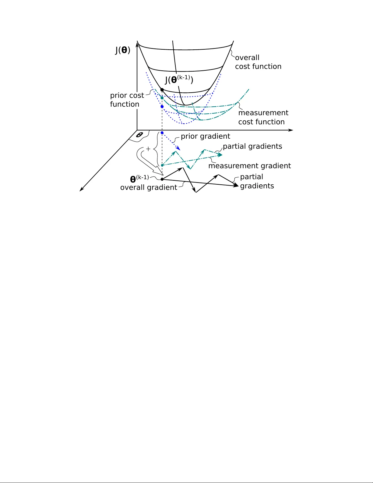
1 Kno wledge-Aided Kaczmarz and LMS Algorithms Michael Lunglmayr*, Oli ver Lang*, and Mario Huemer* Abstract The least mean squares (LMS) filter is often deriv ed via the Wiener filter solution. F or a system identification scenario, such a deri vation mak es it hard to incorporate prior information on the system’ s impulse response. W e present an alternativ e way based on the maximum a posteriori solution, which allows dev eloping a Knowledge-Aided Kaczmarz algorithm. Based on this Knowledge-Aided Kaczmarz we formulate a Knowledge-Aided LMS filter . Both algorithms allow incorporating the prior mean and cov ariance matrix on the parameter to be estimated. The algorithms use this prior information in addition to the measurement information in the gradient for the iterative update of their estimates. W e analyze the con vergence of the algorithms and show simulation results on their performance. As expected, reliable prior information allows improving the performance of the algorithms for low signal-to-noise (SNR) scenarios. The results sho w that the presented algorithms can nearly achiev e the optimal maximum a posteriori (MAP) performance. Index T erms Iterativ e Algorithms, Kaczmarz Algorithm, LMS, MAP , Bayesian estimation, Knowledge-Aided Estimation I . I N T RO D U C T I O N Kno wledge-Aided estimation algorithms hav e a long tradition in digital signal processing, with research areas ranging from generalized Bayesian estimation [1,2] ov er positioning and tar get tracking [3,4] to direction of arriv al estimation [5]–[7]. Ho wev er , to the best of our knowledge, there is no knowledge-aided least mean squares (LMS) filter described in literature, allowing to incorporate prior information on the filter coefficients to be estimated. *Institute of Signal Processing, Johannes Kepler Uni versity Linz, Austria, e-mail: (see www .jku.at/isp/). 2 For the LMS filter , a standard way for deri vation is based on the W iener filter solution [8]– [12]. The W iener filter can be seen as a Bayesian estimator utilizing statistical information on its input x [ k ] , as well as statistical information on the relation of its input to a desired output signal y [ k ] . Its aim is to minimize the mean square error (MSE) between the filter output and the desired output signal, leading to the famous W iener solution [13,14], for the optimal filter coef ficients θ opt : θ opt = R − 1 x x r x y (1) with R x x as the autocorrelation matrix of the input and r x y as the cross-correlation v ector between the input of the W iener filter and the desired output signal. An LMS adaptiv e filter can be seen as a method implicitly approximating R x x and r x y using instantaneous estimates [11]. A prominent applications scenario for adaptiv e filters is system identification [15]. Here the aim is not to optimally estimate the output of the filter but to optimally estimate an unkno wn system with impulse response θ . When considering this scenario, a W iener filter approach makes it hard to incorporate prior kno wledge on θ . As an alternati ve that allows to incorporate such a prior knowledge, we suggest the follo wing way to deriv e the LMS filter . W e first start with a batch based approach and develop a Knowledge-Aided Kaczmarz algorithm. Then we extend the Kaczmarz algorithm to an LMS filter . This e xtension can be easily done due to the arithmetic similarity of the Kaczmarz algorithm and the LMS filter when using the Kaczmarz algorithm with a con volution matrix. Emphasizing its versatility , the presented approach is based on a general linear model that has a widespread application potential: y = H θ + n . (2) The dimensions of H are m × p , of θ are p × 1 and of n and y are m × 1 , respecti vely . The ro ws of H will be denoted as h T i and the elements of y and n as y i as well as n i , ∀ i = 1 , . . . , m , respecti vely . In the general case, H will be an arbitrary system or observ ation matrix, which we assume to ha ve full rank. F or the case of an LMS filter , H will be a con volution matrix with potentially an unlimited number of rows. The vector y is the measurement vector . The parameter vector θ is assumed to be a Gaussian random variable with mean ¯ θ and cov ariance matrix C θθ . These statistics of θ will be used as prior information in the estimation algorithms described belo w . The noise vector n is assumed to be Gaussian as well, with zero mean and 3 cov ariance matrix C nn . In the following deriv ation, we will assume that C nn is a diagonal matrix. W e furthermore assume that C θθ is positi ve definite, which can always be ensured by adding a scaled identity matrix σ I , using a small positive scaling factor σ . This work can someho w be seen as being related to the approach in [16]. There, prior information is used on the model to incorporate systems with missing data. Different to that, we incorporate prior knowledge on the parameter vector to be estimated. Another connection might be drawn to [17], where the author uses a different cost function as we do, incorporating pre vious estimates of the LMS algorithm. Its applications as well as the resulting algorithms are dif ferent to our approach. Another dif ferent approach is used in the Generalized Sidelobe Canceler version of the LMS. There the input signal is altered by a so-called Blocking Matrix to improv e the estimation performance [18]. I I . K N O W L E D G E - A I D E D K AC Z M A R Z A L G O R I T H M In this section, we will deri ve the Kno wledge-Aided Kaczmarz algorithm incorporating the prior information on θ . The idea is to dev elop an iterativ e steepest descent approach similar to Approximate Least Squares (ALS) [19] or the Kaczmarz algorithm [20]. For this, we start with a maximum a posterior (MAP) approach. The deriv ation of the MAP estimator for the model in (2) results in an estimator of the same form as the linear minimum mean square error (LMMSE) estimator [21]. This naturally allows using our algorithms for other use cases of the LMMSE estimator as well. The Knowledge-Aided Kaczmarz algorithm de veloped in this chapter can be seen as an iterativ e v ariant of the batch LMMSE estimator , while the Knowledge-Aided LMS dev eloped below can be seen as an LMS v ariant of an LMMSE estimator using a con volution matrix. A. Derivation via the MAP solution The posterior probability can be calculated as p ( θ | y ) = p ( y | θ ) p ( θ )/ p ( y ) ∝ p ( y | θ ) p ( θ ) . (3) The MAP estimate is the vector ˆ θ MAP = arg max θ p ( y | θ ) p ( θ ) . (4) 4 Here we use ˆ θ to represent an estimate of a true parameter vector θ T . T aking the logarithm and omitting the Gaussian scaling factors giv es: ˆ θ MAP = arg max θ log p ( y | θ ) p ( θ ) (5) = arg max θ − ( y − H θ ) T C − 1 nn ( y − H θ ) − ( θ − ¯ θ ) T C − 1 θθ ( θ − ¯ θ ) (6) Multiplying the cost function with − 1 leads to the optimization problem ˆ θ MAP = arg min θ J ( θ ) (7) with J ( θ ) = ( y − H θ ) T C − 1 nn ( y − H θ ) + ( θ − ¯ θ ) T C − 1 θθ ( θ − ¯ θ ) . This cost function can be split into two parts, a first part ( y − H θ ) T C − 1 nn ( y − H θ ) that we will call measur ement cost function and a second part ( θ − ¯ θ ) C − 1 θθ ( θ − ¯ θ ) that we will call prior cost function . Calculating the partial deriv ativ e of J ( θ ) results in ∇( θ ) = ∂ J ( θ ) ∂ θ = 2 H T C − 1 nn ( H θ − y ) + 2 C − 1 θθ ( θ − ¯ θ ) . (8) This gradient can be used to formulate a steepest descent approach as ˆ θ ( k ) = ˆ θ ( k − 1 ) − µ ∇( ˆ θ ( k − 1 ) ) (9) = ˆ θ ( k − 1 ) − µ  H T C − 1 nn ( H ˆ θ ( k − 1 ) − y ) + C − 1 θθ ( ˆ θ ( k − 1 ) − ¯ θ )  , (10) with the step width µ . F or simplicity , we omitted the factor two of the gradient and assumed that this factor is already included in the step width. An iteration can be formulated via a sum of partial gradients h i w i ( h i T ˆ θ ( k − 1 ) − y i ) + a i C − 1 θθ ( ˆ θ ( k − 1 ) − ¯ θ ) : ˆ θ ( k ) = ˆ θ ( k − 1 ) − µ m Õ i = 1  h i w i ( h i T ˆ θ ( k − 1 ) − y i ) + a i C − 1 θθ ( ˆ θ ( k − 1 ) − ¯ θ )  , (11) with w i as the ( i , i ) t h element of C − 1 nn . The v alues a i are used to bring the gradient of the prior cost function inside the sum, requiring that Í m i = 1 a i = 1 . W e will furthermore assume that a i > 0 , ∀ i = 1 , . . . , m . One ob vious way of fulfilling this condition on the a i v alues is by setting a i = 1 / m , ∀ i = 1 , . . . , m . The cost function as well as its gradients are schematically depicted in Fig. 1. As one can see in this figure, the gradient of the prior cost function redirects the gradient 5 partial gradients θ (k-1) θ J( θ (k-1) ) J( θ ) ^ prior cost funct ion measur ement cost fun ction overall gradient overall cost fun ction prior gra dient partial gr adients measur ement gr adient + Fig. 1: Cost functions and gradients. of the measurement cost function. This allows utilizing the prior information in the gradient based algorithm, improving its performance, as we will show below . The abov e formulation easily allows to use simplifications as done in the ALS [19] or the Kaczmarz algorithm [20], by using only one of the partial gradients per iteration and cyclically re-using the partial gradients after m iterations: ˆ θ ( k ) = ˆ θ ( k − 1 ) − µ k  h k q w k q ( h k q T ˆ θ ( k − 1 ) − y k q ) + a k q C − 1 θθ ( ˆ θ ( k − 1 ) − ¯ θ )  . (12) Here, k q = (( k − 1 ) mod m ) + 1 , represents this cyclic re-use. µ k is the (not necessarily constant) step width used in iteration k . W e will describe ho w to select this step width in more detail in the next section. When using a k q = 1 / m , ∀ k q = 1 , . . . , m , one can see a Bayesian-like characteristic in the partial gradients. The prior information is scaled by one over the number of samples: the more data is collected, the less important the prior information becomes. W e call the iterati ve approach using (12): Knowledge-Aided Kaczmarz . 6 B. Con verg ence of Knowledge-Aided Kaczmarz Using the iteration (12) of Kno wledge-Aided Kaczmarz one can analyze the ev olution of the error e ( k ) = ˆ θ ( k ) − θ T comparing an estimate ˆ θ ( k ) at iteration k to the true parameter vector θ T . Inserting this error in (12) and using y k q = h T k q θ T + n k q gi ves e ( k ) = M k q e ( k − 1 ) + µ k h k q w k q n k q + µ k a k q C − 1 θθ ( θ T − ¯ θ ) , with M k q =  I − µ k  h k q w k q h T k q + a k q C − 1 θθ   . The matrix P k q =  h k q w k q h T k q + a k q C − 1 θθ  consists of a sum of a symmetric and positive semidefinite matrix and a symmetric and positiv e definite matrix. The matrix h k q w k q h T k q has p − 1 eigen values that are zero and one eigen value that is equal to w k q k h k q k 2 2 , corresponding to the eigen vector h k q . C θθ is a cov ariance matrix that we assumed to be positi ve definite, as described in the introduction of this paper . For such a sum of matrices one can easily find limits on its eigen values. For this we define the sequence λ i ( A ) , ∀ i = 1 , . . . , p , as the eigen values of a p × p matrix A in descending order , i.e. λ 1 ( A ) being the largest eigen value, do wn to λ p ( A ) being the smallest eigen v alue. For two symmetric p × p matrices A and B it holds that the maximum eigen value of the sum of matrices, λ 1 ( A + B ) is smaller or equal than the sum of the maximum eigen v alues of the matrices [22]: λ 1 ( A + B ) ≤ λ 1 ( A ) + λ 1 ( B ) . (13) Because we assumed C θθ to be positiv e definite and due to W eyl’ s inequality [22,23] λ i ( A ) + λ p ( B ) ≤ λ i ( A + B ) ≤ λ i ( A ) + λ 1 ( B ) , (14) ∀ i = 1 , . . . , p , it immediately follo ws that the smallest eigen value of P k q must be larger than zero. The aforementioned relations on the eigenv alues can be used to define an interval for µ k limiting the eigen values of M k q . Using 0 < µ k ≤ 1 w k q | | h k q | | 2 2 + a k q λ 1 ( C − 1 θθ ) (15) ensures that all eigen v alues of µ k P k q are smaller or equal than one and lar ger than zero. Consequently , all eigen values of M k q are smaller than one and larger or equal to zero for all k q = 1 , . . . , p . When partitioning (13) into e ( k ) = k Ö i = 1 M i q e ( 0 ) + ∆ k + k − 1 Õ i = 1 ©  « k Ö j = i + 1 M j q ª ® ¬ ∆ i , (16) 7 with ∆ k = µ k  h k q w k q n k q + a k q C − 1 θθ ( θ − ¯ θ )  , we can analyze the error ev olution for k → ∞ . W e denote this error as e (∞) . The initial error vector e ( 0 ) is caused by the start vector θ ( 0 ) of the Kaczmarz iterations. When choosing µ k according to (15), the first product Î k i = 1 M i q e ( 0 ) con ver ges to the zero vector because all eigen values of ev ery M i q are smaller than one, as long as µ is within the bounds of 15. Additionally there are the noise and bias dependent residual terms ∆ k . Because ∆ k is linear in µ , the error e (∞) can be made arbitrary small by selecting a small enough (but lar ger than zero) v alue of µ . Ho we ver , when analyzing the expected value of e (∞) av eraged over n as well as ov er θ one can see that this expected v alue is zero: E n , θ ( e (∞) ) = E n , θ ( ∆ k ) + k − 1 Õ i = 1 ©  « k Ö j = i + 1 M j q ª ® ¬ E n , θ ( ∆ i ) = 0 (17) This sho ws that the Knowledge-Aided Kaczmarz conv erges in the mean. Using the limits on µ k as described abov e, we formulate the follo wing Algorithm 1 that we used for the simulation results presented below . In the beginning, the algorithm uses the upper limits of the interv al in (15) as step widths. For a practical implementation, one would typically pre-calculate these m v alues and store them in a memory . From the iteration where the instantaneous error v k dif fers less than v t h to the error m iterations before, the step width is linearly reduced down to zero with ever y following iteration. For simplicity , v k and v k − m are only compared at iterations when the first ro w of H and the first measurement value from y are used. Such a step width reduction typically leads to a very good performance for Kaczmarz-like algorithms [24]. As pointed out above, for the model (2) the MAP solution is identical to the LMMSE solution. This means LMMSE algorithms, such as the sequential LMMSE [21], could also be used. Ho we ver when analyzing the complexity of LMMSE approaches, e.g. as done in [25], one can see that the complexity of such approaches is typically O ( p 3 ) . For the Kno wledge-Aided Kaczmarz algorithm, the complexity per iteration depends on the matrix C θθ . If C θθ is a full matrix, the comple xity per iteration is O ( p 2 ) , if C θθ is a diagonal matrix, Knowledge-Aided Kaczmarz only has linear complexity per iteration. 8 Algorithm 1 Knowledge-Aided Kaczmarz 1: precalculate C − 1 θθ , λ 1 ( C − 1 θθ ) 2: ˆ θ ( 0 ) ← 0 , v k ← 0 , v k − m ← { largest av ailable number } 3: ReduceMu ← False 4: for k = 1 , . . . , N do 5: v k ← y k q − h T k q ˆ θ ( k − 1 ) 6: if ReduceMu then 7: µ k ← µ k − 1 − µ r 8: else 9: µ k ← 1 w k q | | h k q | | 2 2 + a k q λ 1 ( C − 1 θθ ) 10: if k q = 1 then 11: if | v k − v k − m | < v t h then 12: ReduceMu ← T rue 13: µ k ← 1 max i = 1 , . . ., m ( w i | | h i | | 2 2 + a k q λ 1 ( C − 1 θθ )) 14: µ r = µ k /( N − k + 1 ) 15: end if 16: v k − m ← v k 17: end if 18: end if 19: ˆ θ ( k ) ← ˆ θ ( k − 1 ) + µ k  h k q w k q v k + a k q C − 1 θθ ( ˆ θ ( k − 1 ) − ¯ θ )  20: end for I I I . K N O W L E D G E - A I D E D L M S F I LT E R The Kno wledge-Aided Kaczmarz algorithm can be easily extended to a Knowledge-Aided LMS filter . F or an LMS filter , H has the structure of a con volution matrix, and its number of ro ws m is potentially unlimited. This typically prev ents cyclic re-using of the rows of H as well as the measurement v alues. Equation (11) then potentially requires an infinite series Í ∞ i = 1 a i = 1 . Using the same notation as abov e, the memory of the adaptiv e filter no w becomes the v ector h k and the estimated filter coefficients are ˆ θ ( k ) , resulting in the Knowledge-Aided LMS update equation: ˆ θ ( k ) = ˆ θ ( k − 1 ) − µ k  h k w k ( h k T ˆ θ ( k − 1 ) − y k ) + a k C − 1 θθ ( ˆ θ ( k − 1 ) − ¯ θ )  . Using similar arguments as for the Knowledge-Aided Kaczmarz algorithm, one can see that this algorithm con ver ges in the mean as well. This allows formulating an algorithm similar 9 to Algorithm 1 with the exception that no cyclic re-use of rows is performed because for an LMS filter typically the number of rows of the con volution matrix H is equal to the number of iterations. For simplicity , we also omitted the step-width reduction logic, line 6–18 of Algorithm 1, for the LMS filter and reduced µ k at e very iteration by mulitipling it with ( N − k + 1 )/ N . I V . S I M U L A T I O N R E S U L T S In this section, we show simulation results for the Knowledge-Aided Kaczmarz algorithm as well as for the Kno wledge-Aided LMS filter . For the shown simulations, we alw ays used C θθ = 0 . 1 I and a zero mean vector of the parameter that was to be estimated. For the Kno wledge- Aided Kaczmarz algorithm, we show simulation results for H matrices of dimension 50 × 5 using 500 algorithm iterations. The entries of H have been selected uniformly at random from [ 0 , 1 ] . The obtained results have been av eraged over 100000 simulations. Fig. 2a sho ws the av eraged error norm (over all simulations) at e very iteration of the Knowledge-Aided Kaczmarz algorithm for an SNR= 0 dB. W e also included the simulated MSE performance of the least squares (LS) solution as performance bound for the Kaczmarz algorithm (using the same step width reduction strategy as in Alg. 1) as well as the MSE of the MAP solution as performance bound for the Kno wledge-Aided Kaczmarz algorithm. For the step width reduction of Algorithm 1, v t h was set to 10 − 4 in all Kaczmarz simulations. As one can see from this figure, the Kno wledge-Aided Kaczmarz algorithm is able to utilize the prior information, significantly reducing the final error . Due to the step width reduction, the Kno wledge-Aided Kaczmarz is able to come close to the MAP performance e ven with as little as 500 iterations. Fig. 2b sho ws the final simulated MSE over dif ferent SNR values. As one can see in this picture, the Knowledge Aided Kaczmarz algorithm comes close to the MAP solution for all SNR v alues. As expected, the prior information significantly increases the performance especially at low SNR values. Fig. 4 shows the simulation results for the Kno wledge-Aided LMS filter . Here, we again used 50 measurement values, resulting in m = 50 iterations for the LMS filters. W e estimated a system impulse response of length 5 in a system identification scenario. The input of the LMS filters as well as the unknown systems hav e been selected uniformly at random from [ 0 , 1 ] . W e used a i = 1 / m , ∀ i = 1 , . . . , m , for these simulations. Fig. 3a sho ws the simulated MSE ov er the iterations k for SNR= − 2 dB. As one can see, the prior information significantly improves the performance of the Knowledge-Aided LMS filter as well. Fig. 3b sho ws simulated MSE 10 (a) Performance ov er iterations at SNR = 0 dB. 0 50 100 150 200 250 300 350 400 450 500 10 − 1 10 0 Iteration k avg. ( | | ˆ θ ( k ) − θ | | 2 2 ) Kaczmarz Knowledge-Aided Kaczmarz LS MAP (b) Performance ov er SNR. − 10 − 8 − 6 − 4 − 2 0 2 4 6 8 10 10 − 2 10 − 1 10 0 10 1 SNR avg. ( | | ˆ θ ( 500 ) − θ | | 2 2 ) Kaczmarz Knowledge-Aided Kaczmarz LS MAP Fig. 2: Simulated MSE of Knowledge-Aided Kaczmarz results after 50 iterations of the LMS filter as well as the Knowledge-Aided LMS filter ov er dif ferent SNR values. Again, as expected, the major gains are at low SNR values, if reliable prior information is present. Fig. 3a also allo ws to describe the performance of the Kno wledge-Aided LMS from another point of vie w: is able to achie ve a fix ed performance le vel with a lo wer number of measurements than the con ventional LMS filter . 11 (a) Performance ov er iterations at SNR = − 2 dB. 0 5 10 15 20 25 30 35 40 45 50 10 − 1 10 0 Iteration k avg. ( | | ˆ θ ( k ) − θ | | 2 2 ) LMS filter Knowledge-Aided LMS filter LS MAP (b) Performance ov er SNR. − 10 − 8 − 6 − 4 − 2 0 2 4 6 8 10 10 − 1 10 0 10 1 SNR avg. ( | | ˆ θ ( 50 ) − θ | | 2 2 ) LMS filter Knowledge-Aided LMS filter LS MAP Fig. 3: Simulated MSE of Knowledge-Aided LMS filter . V . C O N C L U S I O N W e presented Knowledge-Aided Kaczmarz and Kno wledge-Aided LMS algorithms that easily allo w utilizing prior information to improv e the performance of the algorithms. W e deriv ed the algorithms via the maximum a posteriori solution. Their con vergence behavior was analyzed, and it was shown that both algorithms con verge in the mean. For low SNR scenarios, the Knowledge- Aided algorithms significantly outperform the standard algorithms. The simulations furthermore sho w that the Knowledge-Aided algorithms are able to achie ve a performance close to the MAP 12 performance. R E F E R E N C E S [1] O. Besson, N. Dobigeon, and J. Y . T ourneret, “Joint Bayesian Estimation of Close Subspaces from Noisy Measurements, ” In IEEE Signal Pr ocessing Letters , V ol. 21, No. 2, pp. 168–171, Feb 2014. [2] A. Amini, U. S. Kamilov , E. Bostan, and M. Unser , “Bayesian Estimation for Continuous-Time Sparse Stochastic Processes, ” In IEEE T ransactions on Signal Processing , V ol. 61, No. 4, pp. 907–920, Feb 2013. [3] J. G. Garcia, P . A. Roncagliolo, and C. H. Mura vchik, “ A Bayesian T echnique for Real and Inte ger Parameters Estimation in Linear Models and Its Application to GNSS High Precision Positioning, ” In IEEE T ransactions on Signal Pr ocessing , V ol. 64, No. 4, pp. 923–933, Feb 2016. [4] A. T urlapaty and Y . Jin, “Bayesian Sequential Parameter Estimation by Cognitive Radar W ith Multiantenna Arrays, ” In IEEE T ransactions on Signal Processing , V ol. 63, No. 4, pp. 974–987, Feb 2015. [5] S. F . B. Pinto and R. C. d. Lamare, “T wo-Step Knowledge-Aided Iterativ e ESPRIT Algorithm, ” In WSA 2017; 21th International ITG W orkshop on Smart Antennas , pp. 1–5, March 2017. [6] Z. Y ang, R. C. de Lamare, X. Li, and H. W ang, “Knowledge-Aided ST AP Using Low Rank and Geometry Properties, ” In International J ournal of Antennas and Pr opagation , pp. 1–14, Aug 2014. [7] X. Zhu, J. Li, and P . Stoica, “Knowledge-aided adaptive beamforming, ” In IET Signal Pr ocessing , V ol. 2, No. 4, pp. 335–345, December 2008. [8] B. W idrow , J. M. McCool, M. G. Larimore, and C. R. Johnson, “Stationary and nonstationary learning characteristics of the LMS adapti ve filter, ” In Proceedings of the IEEE , V ol. 64, No. 8, pp. 1151–1162, Aug 1976. [9] L. Horowitz and K. Senne, “Performance advantage of complex LMS for controlling narrow-band adaptiv e arrays, ” In IEEE T ransactions on Acoustics, Speech, and Signal Pr ocessing , V ol. 29, No. 3, pp. 722–736, Jun 1981. [10] A. Feuer and E. W einstein, “Conv ergence analysis of LMS filters with uncorrelated Gaussian data, ” In IEEE T ransactions on Acoustics, Speec h, and Signal Pr ocessing , V ol. 33, No. 1, pp. 222–230, Feb 1985. [11] S. Haykin, Adaptive F ilter Theory , 4th ed. Upper Saddle Ri ver , NJ: Prentice Hall, 2002. [12] M. Rupp, “The LMS algorithm under arbitrary linearly filtered processes, ” In 19th European Signal Processing Conference , pp. 126–130, Aug 2011. [13] N. W iener , Extrapolation, Interpolation, and Smoothing of Stationary T ime Series . New Y ork NY : W iley , 1949. [14] R. G. Brown and P . Y . C. Hwang, Intr oduction to Random Signals and Applied Kalman F iltering. W ith MATLAB exer cises and solutions , 3rd ed. Ne w Y ork NY : Wile y , 1996. [15] D. G. Manolakis, V . K. Ingle, and S. M. Kogon, Statistical and Adaptive Signal Processing . Norwood, MA: AR TECH HOUSE, 2005. [16] A. Ma and D. Needell, “ Adapted Stochastic Gradient Descent for Linear Systems with Missing Data, ” No. 12, p. 20p, Feb 2017. [Online]. A v ailable: https://arxiv .or g/abs/1702.07098 [17] G. Deng, “Partial update and sparse adaptiv e filters, ” In IET Signal Pr ocessing , V ol. 1, No. 1, pp. 9–17, March 2007. [18] R. K. Miranda, J. P . C. da Costa, and F . Antreich, “High accuracy and low complexity adaptiv e Generalized Sidelobe Cancelers for colored noise scenarios, ” In Digital Signal Pr ocessing , V ol. 34, pp. 48–55, 2014. [19] M. Lunglmayr , C. Unterrieder, and M. Huemer , “ Approximate Least Squares, ” In IEEE International Conference on Acoustics, Speech and Signal Pr ocessing (ICASSP) , pp. 4678–4682, May 2014. 13 [20] S. Kaczmarz, “Przyblizone rozwiazywanie uklad ´ ow r ´ ownan linio wych. – Angen ¨ aherte Aufl ¨ osung von Systemen linearer Gleichungen. ” In Bulletin International de l’Acad ´ emie P olonaise des Sciences et des Lettr es. Classe des Sciences Math ´ ematiques et Natur elles. S ´ erie A, Sciences Math ´ ematiques , V ol. 35, pp. 355–357, 1937. [21] S. M. Kay , Fundamentals of Statistical Signal Pr ocessing: Estimation Theory . Prentice Hall, 1997. [22] T . T ao, T opics in r andom matrix theory . American Mathematical Society , 1997. [23] H. W eyl, “Das asymptotische V erteilungsgesetz der Eigenwerte linearer partieller Dif ferentialgleichungen (mit einer Anwendung auf die Theorie der Hohlraumstrahlung), ” In Mathematische Annalen 71 , No. 4, pp. 441–479, 1912. [24] M. Lunglmayr and M. Huemer, “Parameter Optimization for Step-Adaptive Approximate Least Squares, ” In Computer Aided Systems Theory – EUR OCAST 2015: 15th International Conference , Las P almas de Gran Canaria, Spain, F ebruary 8-13, 2015, Re vised Selected P apers , pp. 521–528, 2015. [25] M. Huemer , A. Onic, and C. Hofbauer, “Classical and Bayesian Linear Data Estimators for Unique W ord OFDM, ” In IEEE T ransactions on Signal Processing , V ol. 59, No. 12, pp. 6073–6085, Dec 2011.