Spectrum Sensing under Spectrum Misuse Behaviors: A Multi-Hypothesis Test Perspective

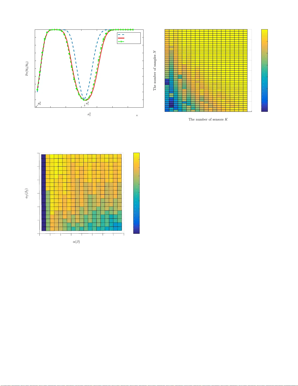
1 Spectrum Sensing under Spectrum Misuse Beha viors: A Multi-Hypothesis T est Perspecti v e Linyuan Zhang, Guoru Ding, Senior Member , IEEE , Qihui W u, Senior Member , IEEE , and Zhu Han, F ellow , IEEE Abstract —Spectrum misuse behaviors, brought either by il- legitimate access or by rogue po wer emission, endanger the legitimate communication and deteriorate the spectrum usage en vironment. In this paper , our aim is to detect whether the spec- trum band is occupied, and if it is occupied, r ecognize whether the misuse behavior exists. One vital challenge is that the legitimate spectrum exploitation and misuse beha viors probabilistically co- exist and the illegitimate user (IU) may act in an intermittent and fast-changing manner , which brings about much uncertainty for spectrum sensing . T o tackle it, we firstly f ormulate the spectrum sensing problems under illegitimate access and rogue power emission as a unif orm ternary hypothesis test. Then, we develop a novel test criterion, named the generalized multi-hypothesis Neyman-Pearson (GMNP) criterion. F ollowing the criterion, we derive two test rules based on the generalized likelihood ratio test (GLRT) and the Rao test, respectively , whose asymptotic performances are analyzed and an upper bound is also given. Furthermore, a cooperative spectrum sensing scheme is designed based on the global GMNP criterion to further impro ve the detection performances. In addition, extensive simulations are pro vided to verify the proposed schemes’ performance under various parameter configurations. I . I N T RO D U C T I O N A. Backgr ound and Motivation Due to the explosiv e growth of wireless devices and ser- vices, the scarceness of spectrum resources has become more and more serious. Dynamic spectrum sharing has been well recognized as a promising approach to impro ve the spectrum utilization and reliev e the spectrum shortage [1]–[3]. Howe ver , it may put the future at risk brought by various attacks [4], [5], among which spectrum misuse behaviors have recei ved increasingly wide attention. Generally , spectrum misuse be- haviors refer to the manner of exploiting spectrum that violates This work is supported by the National Natural Science Foundation of China (Grant No. 61501510 and No. 61631020), Natural Science Foundation of Jiangsu Province (Grant No. BK20150717), Natural Science Foundation for Distinguished Y oung Scholars of Jiangsu Province under Grant (No. BK20160034), and in part by US NSF CNS-1717454, CNS-1731424, CNS- 1702850, CNS-1646607, ECCS-1547201, CMMI-1434789, CNS-1443917, and ECCS-1405121. L. Zhang and G. Ding are with the College of Communications Engineering, Army Engineering University of PLA, Nanjing 210007, China (e-mail: zhanglinyuan5@163.com, dr.guoru.ding@ieee.or g). G. Ding is also with the National Mobile Communications Research Laboratory , Southeast Uni versity , Nanjing 210018, China. Q. Wu is with the Department of Electronics and Information Engineering, Nanjing University of Aeronautics and Astronautics, Nanjing 210007, China (email: wuqihui2014@sina.com). Z. Han is with the Univ ersity of Houston, Houston, TX 77004 USA (e- mail:zhan2@uh.edu), and also with the Department of Computer Science and Engineering, Kyung Hee University , Seoul, South Korea. L i c e n s e d u s e r I l l e g a l u s e r F u s i o n c e n t e r S e n s o r s L e g i t i m a t e u s e r ( LU ) I l l e g i t i m a t e u s e r ( IU ) F u s i o n c e n t e r ( FC ) S e n s o r s LU FC LU / IU FC IU S e n s o r s S e n s o r s . . . . . . (a) Illegitimate access L i c e n s e d u s e r I l l e g a l u s e r F u s i o n c e n t e r S e n s o r s L e g i t i m a t e u s e r ( LU ) I l l e g i t i m a t e u s e r ( IU ) F u s i o n c e n t e r ( FC ) S e n s o r s LU FC LU / IU FC IU S e n s o r s S e n s o r s . . . . . . (b) Rogue po wer emission Fig. 1: Spectrum misuse behaviors and a distrib uted detection framew ork. Dotted lines denote the received signal of sensors due to the probabilistic emission behaviors of the IU and the legitimate user (LU), while the solid lines denote that sensors report decisions to the fusion center (FC). the spectrum regulations. As illustrated in Fig. 1, two typical spectrum misuse behaviors are as follows: • Ille gitimate access launched by external attackers, just as shown in Fig. 1 (a). One example is the primary user emulation (PUE) attack [6]–[9] that launches the denial of service (DoS) attack, where the illegitimate user emulates the characteristics of the primary user’ s signal when the sensors conduct spectrum sensing in order to prev ent the secondary users from accessing the idle spectrum [10]–[13]. Another example is the fake or rogue access point (AP) that disguises as an authorized AP by spoofing the authorized AP’ s medium access control (MA C) address in order to lure users to connect to them [14] [15]. In addition, the illegitimate access can be done indirectly through launching data falsification attacks in the cooperative spectrum sensing [16] [17], where the global decisions are misled and as a result, collisions between secondary users and the primary user increase and attackers illegitimately access the idle channel [18], [19]. • Rogue power emission taken by internal attackers, just as shown in Fig. 1 (b). In some cases, a selfish attack er may break the upper bound of the transmit power constraint for a higher data rate [20] [21]. Similarly , some malicious attackers may intentionally apply for spectrum exploita- tion with a large coverage, quoting a high transmit power , but in fact they work with a low transmit power , which decreases the spectrum ef ficiency of spatial reuse [22]. The internal attackers have obtained the authorization of the usage of the spectrum, and as a result, this kind of 2 misuse behaviors is stealthier . These spectrum misuse behaviors lead to serious inter- ference with the legitimate communication and disordered spectrum usage environment, which poses a fundamental re- quirement on the detection of these misuse behaviors. B. Related W ork Spectrum misuse behaviors pose direct influences on the channel states, while spectrum sensing plays a vital role in obtaining the real-time channel states. Further , considering the high feasibility , spectrum sensing based methods hav e been exploited in the detection of spectrum misuse behaviors [12], [20], [23]–[25]. Specifically , the detection problem of the illegitimate access is formulated as a statistical significance test between the normal usage and the abnormal one in [25], where the normal usage is defined as being no more than one transmitter working in each portion (e.g., channel) of the spectrum. But, it can’t find out the case that only the IU works. T o tackle this problem, [12] introduces the spectrum policy maker to obtain the factual state of the LU, based on which the detection is divided into two cases, i.e., when the LU isn’ t working and when the LU is working. Especially , when the existence of the IU taking illegitimate access is prior known, an optimal combining scheme is proposed for cooperati ve spectrum sensing (CSS) in [23]. Differently , considering the assumption that no more than one user, either the LU or the IU, works on a spectrum band of interest during one slot, [24] proposes a fingerprints-power -belief based noncentral detection algorithm through making power estimation and calculating the compatibility in a distributed manner . On the other side, fe w works hav e been done for the rogue power emission problem. In [20], crowdsourced enforcement, where a crowd of mobile users collaterally make detection, is exploited to find out the spectrum misuse behavior and the related characteristics, e.g., the signal strength, are analyzed. In fact, one basic but vital problem is that the detectors gen- erally hav e no ground truth of either the legitimate exploitation or misuse beha viors. Hence, in this paper , we focus on two new features about the sensing model: • F r om binary-hypothesis to multi-hypothesis : W e not only identify whether the spectrum band is occupied or not, b ut also ha ve to mak e clear whether the band, if occupied, is occupied legitimately or illegitimately . Due to lack of the ground truth about the LU’ s behaviors, the traditionally binary-hypothesis test model is inaccurate to characterize the ne w problem any more. Hence, considering the prob- abilistic coexistence of the IU and the LU, it is essential to formulate the detection problem as a multi-hypothesis test problem. • F r om simple hypothesis to composite hypothesis : From the perspectiv e of protecting itself from being detected, the IU may behav e in an intermittent and fast-changing manner . As a result, it is hard to obtain the accurate parameters of the IU, such as the transmit po wer and channel gains, which means that the composite hypothe- ses with a family of distributions are needed to formulate the behaviors instead of simple ones with a single distri- bution. T o the best of the authors’ knowledge, there is no work considering the detection of spectrum misuse behaviors as a multi-hypothesis test consisting of simple hypotheses and composite hypotheses, though multiple hypotheses and com- posite hypotheses have been separately considered in current work about spectrum sensing. In [26], the case that the licensed user works on more than one discrete transmit power levels is considered and a multi-hypothesis test is made to detect the existence of the signal and recognize the power levels based on the maximum a posterior rule. Further , for the same multi-power -level case, a sequential detection is studied based on the modified Neyman-Pearson (NP) rule in [27]. As the transmit power lev els are deterministic and known for the sensors, all hypotheses are simple. Ho wev er , when some key parameters are unknown, the hypothesis becomes composite. In [28], a two-sided parameter testing problem is analyzed, where the user’ s transmitting power and the position are unknown, and a generalized Rao test is deriv ed for the binary hypothesis test consisting of a simple hypothesis and a composite one. Nevertheless, this paper formulates a different multiple hypothesis test, which consists of composite hypotheses and simple ones, and the problem is complex and hard to obtain an optimal scheme. C. Contributions In this paper , a distributed detection framew ork is built, where e very sensor makes spectrum sensing and local deci- sion, and based on the decisions recei ved from the sensors, the FC makes data fusion and global decision, just as shown in Fig. 1. Our aim is to detect whether the channel is occupied, and if it is occupied, recognize whether the IU exists. The main contributions are summarized as follows: • W e firstly formulate the spectrum sensing problem under illegitimate access and rogue power emission as multi- hypothesis tests, respectively , where the states without the IU are modeled as simple hypotheses and the states with the IU are modeled as composite ones due to the unknown characteristics about the IU, and gi ve a uniform model for the two cases, i.e., a ternary hypothesis test, through certain transformation to facilitate the analysis and processing. • W e propose a generalized multi-hypothesis Neyman- Pearson (GMNP) criterion and deri ve the test rule. Specif- ically , in the GMNP criterion, the detection probability about spectrum misuse behaviors is maximized under two constraints about the detection probabilities of states without the IU. Following the criterion, two test rules are deriv ed based on the GLR T and the Rao test, respectively . In particular , due to the multi-hypothesis characteristic, the overlapping problem of decision regions is analyzed and the solution is given. T o ev aluate the proposed schemes, the asymptotic performance is deriv ed and an upper bound of the detection performance is also giv en. • W e design a cooperativ e spectrum sensing (CSS) scheme for the ternary hypothesis test based on the global GMNP 3 T ABLE I: Ke y notations and symbols used in this paper . Symbol Definition LU The legitimate user I U The illegitimate user Pr( · ) the probability of certain ev ent F ( · ) the probability distribution function of certain parameter p ( · ) the probability density function of certain parameter H i the hypothesis H i , i ∈ { 0 , 1 , 2 } R i the corresponding decision region of H i N the number of samples K the number of sensors test criterion. Due to the unkno wn detection performance when the IU exists, the criterion is further transformed, based on which a data fusion-based CSS algorithm is dev eloped. • W e present in-depth simulations to verify the detection performance versus the unknown parameter , the number of sensors, and the number of samples in two scenarios: sensing with one single sensor and sensing with multiple sensors. Notably , the proposed method can handle with both ille- gitimate access and rogue power control from the perspective of spectrum sensing. Considering that current works focus on either the ille gitimate access or rogue power control, our work shows high efficiency . D. Or ganization and Notation The rest of this paper is organized as follows. The system model under spectrum misuse behaviors is formulated in Section II. Section III formulates the GMNP criterion, derives the test rule, and gives an upper bound of the detection performance. Cooperative spectrum sensing is analyzed in Section IV . Simulation is giv en in Section V , followed by the conclusion in Section VI. The proofs of all theorems are gi ven in the appendix. T o facilitate the reading, the key notations are summarized in T able I. I I . S Y S T E M M O D E L U N D E R S P E C T R U M M I S U S E B E H A V I O R S A. Pr oblem F ormulation Con ventionally , to detect whether a LU is transmitting signals in a given spectrum band, a binary hypotheses test is carried out between the null hypothesis L 0 (the LU is absent) and the alternative hypothesis L 1 (the LU is present) [30]: L 0 : y L ( t ) = n ( t ) , L 1 : y L ( t ) = p P s s ( t ) + n ( t ) , (1) where y L ( t ) is the receiv ed signal of a sensor in time slot t , s ( t ) is the signal transmitted by the LU, P s is the receiv ed power that is related with the transmit power and the path loss and inv ariable during the observation time, and n ( t ) is the additiv e Gaussian white noise with the variance σ 2 n . Further , to facilitate the analysis, in the following, s ( t ) is assumed to be an independent and identically distributed (i.i.d.) random process with zero mean and unit variance, i.e., s ( t ) ∼ N (0 , 1) [23] [31]. Here, P s and σ 2 n are assumed to be prior known, and it is considered from two aspects: it is wise for the LU to provide some information (such as the transmit power and statistical channel state) to assist sensors of well finding out the mis-behav ed IU [12]; considering the LU’ s regularity compared with the IU’ s burstiness, it is feasible to estimate the received power P s of the LU and the noise σ 2 n ov er a long observation. Hence, in L 1 , y L ( t ) ∼ N (0 , P s + σ 2 n ) . Over a sensing slot T , the sensor obtains N samples, y = ( y 0 , y 1 , ..., y N ) , based on which the test is done. Next, we analyze two cases of spectrum misuse behaviors, illegitimate access and rogue power control, respectiv ely . 1) Ille gitimate access: In this case, the IU is an unau- thorized user taking illegitimate access, and another binary hypotheses test about the IU can be modeled as follows: I 0 : y I ( t ) = 0 , if no IU exists; I 1 : y I ( t ) = p P x x ( t ) , if an IU exists. (2) where y I ( t ) is the illegitimate component in the receiv ed signal, and x ( t ) is the signal transmitted by the IU with the received power P x . As the IU always imitates the signal characteristics of the LU to hide itself from being detected, x ( t ) is also assumed to be an i.i.d. random process with zero mean and unit v ariance, i.e., x ( t ) ∼ N (0 , 1) . In addition, as the IU generally works abruptly in a non-cooperativ e manner with the detection system in order to better hide itself from being detected, P x is hard to obtain. Nevertheless, considering the short sensing time and the ignorable, P x is assumed to be in variable during one sensing slot. Furthermore, let P ( L i ) and P ( I j ) , i, j ∈ { 0 , 1 } , denote the prior probabilities about the existence of the LU and the IU, respectiv ely . W e hav e Pr( L i , I i ) = P ( L i ) Pr( I i |L i ) . (3) Remark. The dependence of the IU’ s states and the LU’ s states varies with differ ent goals and the prior information. In the case that the IU aims to well exploit the spectrum for fr ee, e.g., the PUE attack, it pr efers to work when the LU is absent and Pr( I 1 |L 0 ) may be higher than Pr( I 1 |L 1 ) . While in another case that the IU’s goal is to deteriorate normal communication of the LU, e.g., the jamming attack, Pr( I 1 |L 1 ) may be higher than Pr( I 1 |L 0 ) . Howe ver , it is generally hard to obtain accur ate information about the states of the LU for the IU. In an extr eme case that ther e is no information about the r eal state of the LU, the IU has to work completely randomly and independently , i.e., Pr( L i , I i ) = P ( I i ) P ( L i ) . 2) Rogue power contr ol: In this case, the IU is the au- thorized user working with a lower or higher transmit power than the quoted v alue, and the corresponding state can be formulated as follows: L 2 : y L ( t ) = p δ · P s s ( t ) + n ( t ) , δ ∈ (0 , 1) ∪ (1 , ∞ ) . (4) The metric δ reflects the tendency of the IU and the seriousness of the illegitimate behaviors. δ > 1 indicates that the IU aims 4 to enhance its own communication and bring the neighbors more interference, while δ < 1 indicates that the IU aims to occupy the channel ov er a large area and prev ent other users of taking access to the channel in the area. It is noted that in this case, only one user exists. If the user is w orking on the channel, it is either the LU or the IU during one slot. It is different from the case of illegitimate access, in which the LU and the IU are two entities. This difference will be apparently reflected in the modeling process below . B. Pr eliminary Spectrum Sensing Model: Composite Hypoth- esis T ests 1) Spectrum sensing model under ille gitimate access: Considering the probabilistic co-existence of the LU and the IU, the spectrum sensing problem under illegitimate access behaviors is formulated as a quaternary hypothesis test: S 0 : y ( t ) = n ( t ) , S 1 : y ( t ) = p P s s ( t ) + n ( t ) , S 2 : y ( t ) = p P x x ( t ) + n ( t ) , S 3 : y ( t ) = p P s s ( t ) + p P x x ( t ) + n ( t ) , (5) where S 0 , S 1 , S 2 , and S 3 denote the states that no users exist, only the LU e xists, only the IU exists, and the IU and the LU co-exist, respectively , and y ( t ) is the observation of a certain sensor at the t -th slot. Based on the signal characteristics, the dif ference among the hypotheses, in the vie w of the sensor , is the observ ation value’ s variance. Specifically , y ∼ N (0 , σ 2 ) , where the parameter σ 2 is σ 2 n , ( P s + σ 2 n ) , ( P x + σ 2 n ) , and ( P s + P x + σ 2 n ) , under the hypotheses S 0 , S 1 , S 2 , and S 3 , respecti vely . Notably , P x is unknown and due to the superposition of the LU’ s signal and the IU’ s signal in S 3 , we have σ 2 > σ 2 1 . Hence, the test can be rewritten as follows: S 0 : σ 2 = σ 2 0 , S 1 : σ 2 = σ 2 1 , S 2 : σ 2 > σ 2 0 and σ 2 6 = σ 2 1 , S 3 : σ 2 > σ 2 1 , (6) where σ 2 0 = σ 2 n , σ 2 1 = P s + σ 2 n . Here, S 0 and S 1 are simple hypotheses whose parameter is a single value, while S 2 and S 3 are composite ones whose parameter’ s value space is a set. In S 2 , σ 2 6 = σ 2 1 is set to distinguish S 2 from S 1 . In fact, in S 2 , the value of σ 2 is continuous so that the probability of σ 2 = σ 2 1 is zero, which means that it poses few ef fects on the results of the test. Furthermore, let p ( P x ) denote the probability density func- tion of the receiv ed power from the IU. Then, the probability distribution function F ( σ 2 ) of the variance σ 2 is F ( σ 2 ) =              0 , σ 2 < σ 2 0 , a 00 , σ 2 = σ 2 0 , a 00 + a 01 R σ 2 − σ 2 0 0 p ( P x ) dP x , σ 2 0 < σ 2 < σ 2 1 , a 00 + a 10 + a 01 R σ 2 1 − σ 2 0 0 p ( P x ) dP x , σ 2 = σ 2 1 , F ( σ 2 1 ) + a 11 R σ 2 − σ 2 1 0 p ( P x ) dP x , σ 2 > σ 2 1 , (7) 2  2 1  0  2 0  1  2  3  0 0  1  2  ... 2  2 1  2 0  0 ... Fig. 2: Spectrum sensing under illegitimate access: A quaternary-hypothesis test. where a ij = P ( L i , I j ) . Then, we hav e the probability density function of the observation value: p ( y i ) = Z + ∞ σ 2 0 1 √ 2 π σ 2 e − y 2 i 2 σ 2 dF ( σ 2 ) , (8) where i ∈ { 1 , 2 , ..., N } . 2) Spectrum sensing model under the r ogue power contr ol: Based on (1)(4), there are three channel states under the rogue power control, and correspondingly , the spectrum sensing problem can be modeled as a ternary hypothesis test: L 0 : σ 2 = σ 2 0 , L 1 : σ 2 = σ 2 1 , L 2 : σ 2 = σ 2 0 + δ ( σ 2 1 − σ 2 0 ) , δ ∈ (0 , 1) ∪ (1 , ∞ ) . (9) Here, both the metric δ and its distrib ution are unkno wn, which means that the hypothesis L 2 is composite. 3) Summary: The two cases are different in many aspects, such as external/internal attacks, one/two entities entity , and attack objectives. Howe ver , from the perspectiv e of spectrum sensing, the two kinds of spectrum misuse behaviors show much similarity: • Both the tests consist of simple hypotheses without the IU and composite hypotheses with the IU. • There are unknown parameters in both cases, i.e., the receiv ed po wer from the IU P x and the metric δ , and though the parameters are different, they pose effects on spectrum sensing through the variances of the observa- tions. In the following, we will find that the two cases can be uniformly modeled through certain reasonable transformation. C. Uniform Spectrum Sensing Model: A T ernary Hypothesis T est Firstly , in the case of illegitimate access, though the qua- ternary hypothesis test in (6) gives the general formulation about the spectrum sensing problem under ille gitimate access, the prior kno wledge, such as the prior probabilities and the distribution of P x , is hard to obtain and the equations (7)(8) cannot be calculated. Furthermore, the hypothesis S 2 with the variance σ 2 > σ 2 0 , σ 2 6 = σ 2 1 , and the hypothesis S 3 with the variance σ 2 > σ 2 1 are partly ov erlapping, just as sho wn in Fig. 2. As a result, it is hard to distinguish the two states. T o tackle the problems above, we transform the original quaternary hypothesis test about the illegitimate access to a ternary hypothesis test. The key rational is that our objective is to detect whether the channel is occupied and if it is occupied, 5 recognize whether the IU exists, where the first part is to find out the spectrum holes, while the second part is to protect the scare resource of spectrum from being used illegitimately . T o achieve the former part, S 0 ought to be distinguished from the other hypotheses, while to achiev e the latter one, the hypotheses S 0 and S 1 ought to be distinguish from the other two hypotheses S 2 and S 3 . Hence, the objectiv e can be achiev ed, ev en though the two hypotheses S 2 and S 3 are not distinguished. That is to say , we can combine S 2 and S 3 in one hypothesis, i.e., σ 2 ∈ ( σ 2 0 , σ 2 1 ) ∪ ( σ 2 1 , + ∞ ) . Here, we find that the new hypothesis in the case of illegitimate access is identical to L 2 , i.e., the hypothesis of the IU launching rogue power control. Consequently , the two cases can be uniformly modeled as a ternary hypothesis test:      H 0 : σ 2 = σ 2 0 , H 1 : σ 2 = σ 2 1 , H 2 : σ 2 ∈ ( σ 2 0 , σ 2 1 ) ∪ ( σ 2 1 , + ∞ ) , (10) where the simple hypotheses H 0 and H 1 denote that the channel is idle and the channel is occupied by the LU, respectiv ely , while the composite hypothesis H 2 means that the IU exists, in which the IU can launch illegitimate access or rogue po wer control, and σ 2 2 is used to denote the unknown variance of the observation in H 2 . I I I . T H E G E N E R A L I Z E D M U LT I - H Y P O T H E S I S N E Y M A N - P E A R S O N C R I T E R I O N A N D T H E T E S T RU L E In this section, based on the proposed ternary-hypothesis testing model, a novel test criterion called the GMNP criterion is proposed and the test rule is derived, which is decomposed into two subproblems: a detection subproblem and a recog- nition subproblem. Then, the mutual ef fects between the two parts are analyzed. Finally , the upper bound of the detection performance is derived with the prior knowledge of the range of the unknown parameter . A. The Generalized Multi-Hypothesis Neyman-P earson Crite- rion In the ternary hypothesis model, not only the prior prob- abilities are unknown, but also the prior distribution of σ 2 2 is hard to obtain. Moreo ver , it is conflicting to impro ve the detection probabilities of all hypotheses simultaneously . T o tackle these issues, we build an optimization criterion named the generalized multi-hypothesis Neyman-Pearson (GMNP) criterion, where the probability of correctly identifying misuse behaviors, Pr( H 2 |H 2 ) , is maximized, subjected to the con- straints on the detection probabilities about H 0 and H 1 (i.e., Pr( H 0 |H 0 ) and Pr( H 1 |H 1 ) ), which is formulated as follows: max R 0 , R 1 , R 2 Pr( H 2 |H 2 ) , s.t. Pr( H 0 |H 0 ) ≥ α, Pr( H 1 |H 1 ) ≥ β , (11) where Pr( H i |H j ) , i, j ∈ { 0 , 1 } denotes the probability of the decision H i being made when the real state is H j , and α and β are constants which play as the constraints on the basic test performance, 0 . 5 < α < 1 , 0 . 5 < β < 1 . In addition, R i denotes the decision region of H i , that is, Pr( H i |H j ) , Z R i p ( y ; H j ) d y , where p ( y ; H j ) is the probability density function of the observation sequence y under H j . Furthermore, we equi valently simplify the optimization cri- terion based on Lemma 1. Lemma 1. The optimization criterion in (11) is equivalent to the one below: max R 0 , R 1 , R 2 Pr( H 2 |H 2 ) , (12a) s.t. Pr( H 0 |H 0 ) = α, (12b) Pr( H 1 |H 1 ) = β . (12c) Remark. In the traditional Neyman-P earson criterion of the binary-hypothesis test, the detection pr obability about the alternative hypothesis is maximized with the constraint of the false alarm probabili ty about the null hypothesis [32]. Hence, the GMNP criterion in (11) and (12) can be r e gar ded as an extension of the Neyman-P earson criterion in the generalized multi-hypothesis test. Nevertheless, the main differ ences focus on one point: the multi-hypothesis test encounter s the compos- ite hypothesis. Multiple hypotheses incr eases the complexity of carving out the decision re gions, while the composite hypothesis raises its difficulty . In the following, we focus on designing the test rule. B. The Pr oposed T est Rule Firstly , to maximize the detection probability about spec- trum misuse behaviors under the giv en detection probabilities of H 0 and H 1 , we use the Lagrange multiplier method to construct the objective function: F = Pr( H 2 |H 2 ) + λ 0 (Pr( H 0 |H 0 ) − α ) + λ 1 (Pr( H 1 |H 1 ) − β ) . (13) Further , we have F = 1 − Z R 0 p ( y ; H 2 ) d y − Z R 1 p ( y ; H 2 ) d y + λ 0 ( Z R 0 p ( y ; H 0 ) d y − α ) + λ 1 ( Z R 1 p ( y ; H 1 ) d y − β ) = Z R 0 [ λ 0 p ( y ; H 0 ) − p ( y ; H 2 )] d y + Z R 1 [ λ 1 p ( y ; H 1 ) − p ( y ; H 2 )] d y + 1 − λ 0 α − λ 1 β . (14) In (14), we find that to maximize F , in the decision region R 0 , λ 0 p ( y ; H 0 ) − p ( y ; H 2 ) > 0 , while in the decision region R 1 , λ 1 p ( y ; H 1 ) − p ( y ; H 2 ) > 0 , where the two constants λ 0 and λ 1 are decided to satisfy the constraints in (12). Furthermore, 6 to maximize Pr( H 2 |H 2 ) , H 2 is decided when p ( y ; H 2 ) p ( y ; H 0 ) > λ 0 , (15a) p ( y ; H 2 ) p ( y ; H 1 ) > λ 1 . (15b) It is shown that to achiev e the GMNP criterion in (11) and (12), two lik elihood ratios p ( y ; H 2 ) p ( y ; H 0 ) and p ( y ; H 2 ) p ( y ; H 1 ) are used in the detection process. Put (12) and (15) together , and we find that the constraint in (12b) is related to the former likelihood ratio which includes H 0 and H 2 , while the other constraint in (12c) is related to the latter one which includes H 1 and H 2 . Hence, the optimization problem in (12) can be decomposed into two subproblems, which are formulated as follows: max R 0 , R 2 Pr( H 2 |H 2 ) , s.t. Pr( H 0 |H 0 ) = α, (16) and max R 1 , R 2 Pr( H 2 |H 2 ) , s.t. Pr( H 1 |H 1 ) = β , (17) respectiv ely , where the final solution of R 2 is the intersection of the solutions of the two subproblems. Hence, through the decomposition above, we simplify the former problem. More importantly , we find that the two subproblems have clear physical significance, based on which the two subproblems are named the detection subproblem and the recognition subproblem. 1) Detection subpr oblem (Idle or busy): The first sub- problem in (16) can be thought to stem from such a binary hypothesis test: H 0 : σ 2 = σ 2 0 , H 2 : σ 2 > σ 2 0 , and σ 2 6 = σ 2 1 . (18) Let σ 2 denote the variance of the observ ation value under H 2 , and as σ 2 2 > σ 2 0 , this problem is single-side. Then, to maximize Pr( H 2 |H 2 ) while constraining Pr( H 0 |H 0 ) to be α , we exploit the likelihood ratio test (LR T): L 0 ( y ) = p ( y ; H 2 ) p ( y ; H 0 ) = 1 (2 π σ 2 2 ) N 2 exp( − P N − 1 n =0 y 2 n 2 σ 2 2 ) 1 (2 π σ 2 0 ) N 2 exp( − P N − 1 n =0 y 2 n 2 σ 2 0 ) =  σ 2 0 σ 2 2  N 2 exp  σ 2 2 − σ 2 0 2 σ 2 0 σ 2 2 X N − 1 n =0 y 2 n  H 2 R H 0 λ 0 . (19) As y works in the manner of P N − 1 n =0 y 2 n in (19), the test statistic is Y = P N − 1 n =0 y 2 n . L 0 ( y ) increases with Y , as σ 2 2 > σ 2 0 . Hence, to mak e L 0 ( y ) < λ 0 means that Y < η 0 , where η 0 is the corresponding threshold to λ 0 . Further , under H 0 , Y = P N − 1 n =0 y 2 n ∼ χ 2 N ( σ 2 0 ) . Hence, we have Pr( H 0 |H 0 ) = Pr( Y < η 0 |H 0 ) = 1 − Γ( N 2 , η 0 σ 2 0 ) Γ( N 2 ) = α, (20) where Γ( · ) and Γ( · , · ) are the Gamma function and upper incomplete Gamma function, respecti vely . Hence, the decision threshold is derived as η 0 = Γ − 1  N 2 , (1 − α ) Γ( N 2 )  σ 2 0 , (21) where Γ − 1 ( · , · ) is the in verse incomplete Gamma function. Hence, the test rule for the detection subproblem is Y H 2 R H 0 η 0 . (22) 2) Recognition subpr oblem (Legitimate or ille gitimate): The second subproblem (17) can be thought to stem from such a binary hypothesis test: H 1 : σ 2 = σ 2 1 , H 2 : σ 2 > σ 2 0 , and σ 2 6 = σ 2 1 . (23) Different from the detection subproblem, the recognition subproblem is double-side, i.e., the unknown variance σ 2 2 may be either higher or lower than σ 2 1 . Next, we apply the GLR T to tackle with the double-side problem. Then, asymptotic analysis is made about the detection performance. T o bypass the complexity of obtaining the thresholds in the GLR T , another scheme, i.e., the Rao test, is also deriv ed. a) GLRT : First, we calculate the unknown v ariance’ s maximum likelihood estimation (MLE) ˆ σ 2 2 of σ 2 2 : ˆ σ 2 2 = arg max σ 2 2 p ( y ; σ 2 2 ) . (24) Let ∂ p ( y ; ˆ σ 2 2 ) ∂ ˆ σ 2 2 = 0 , and we have ˆ σ 2 2 = 1 N X N − 1 n =0 y 2 n . (25) Further , we have the likelihood ratio L 1 = p ( y ; ˆ σ 2 2 , H 2 ) p ( y ; H 1 ) = N σ 2 1 P N − 1 n =0 y 2 n ! N 2 exp P N − 1 n =0 y 2 n 2 σ 2 1 − N 2 ! H 2 R H 1 λ 1 . (26) As the test statistic Y is P N − 1 n =0 y 2 n , L 1 is the function of Y and we have dL 1 d Y = 1 2  N σ 2 1 Y  N 2 e Y 2 σ 2 1 Y − N σ 2 1 Y σ 2 1 . (27) Therefore, when Y > N σ 2 1 , L 1 increases with Y ; otherwise, L 1 decreases with Y . Hence, the minimum of the likelihood ratio is achieved at N σ 2 1 and λ 1 > 1 . Thus, L 1 < λ 1 is equiv alent to η 1 < Y < η 2 , where η 1 and η 2 are two solutions of L 1 ( Y ) = λ 1 , i.e.,  N σ 2 1 η 1  N 2 exp( η 1 2 σ 2 1 − N 2 ) =  N σ 2 1 η 2  N 2 exp  η 2 2 σ 2 1 − N 2  = λ 1 . (28) 7 Simultaneously , when only the LU does exist, i.e., H 1 , Y = P N − 1 n =0 y 2 n ∼ χ 2 N ( σ 2 1 ) and the condition below is satisfied: Pr( H 1 |H 1 ) = Pr( η 1 < Y < η 2 ) = Γ( N 2 , η 1 σ 2 1 ) − Γ( N 2 , η 2 σ 2 1 ) Γ( N 2 ) = β . (29) Hence, based on (28) and (37), the two thresholds η 1 and η 2 can be obtained. Finally , the test rule in this part is formulated as follows:  H 1 is declared , if η 1 < Y < η 2 , H 2 is declared , otherwise. (30) b) Asymptotic analysis: Considering the complexity of the GLR T , the thresholds are hard to be formulated in the closed-form manner . Nevertheless, when the number of sam- ples is sufficiently large, some approximation can be made and the asymptotic performance (i.e., N → ∞ ) is analyzed. Proposition 1. When N is sufficiently larg e and the channel is occupied by the LU, we have 2 ln L 1 a ∼ χ 2 1 . Then, let z 2 = 2 ln L 1 , where z follows a Gaussian distribution with mean zero and variance 1, i.e., z ∼ N (0 , 1) , and we have Pr( H 1 |H 1 ) a = Pr(2 ln L 1 < 2 ln λ 1 |H 1 ) = Z √ 2 ln λ 1 − √ 2 ln λ 1 1 √ 2 π ρ z 2 2 dz = 2 Q ( − p 2 ln λ 1 ) − 1 = β , (31) where Q ( · ) is the complementary distribution function of the standard Gaussian. Hence, we can obtain the asymptotic solution of λ 1 as follows λ 1 a = exp " 1 2  Q − 1 ( 1 + β 2 )  2 # . (32) In addition, based on (28), the approximate values of η 1 and η 2 are obtained. Though the complexity of calculating the thresholds de- creases, we still cannot obtain the closed-form expressions of the thresholds, which makes it not easy to e valuate the test performance. Nevertheless, we make another proposition below so that we can ev aluate the asymptotic performance. Proposition 2. When N is sufficiently lar ge and the hypothesis H 2 is true, z 2 = 2 ln L 1 ( y ) a ∼ χ 0 2 1 ( θ ) , z ∼ N ( √ θ , 1) , where χ 0 2 1 ( θ ) is a noncentral chi-squar e distribution with the noncen- tral parameter θ = ( σ 2 2 − σ 2 1 ) 2 I ( σ 2 1 ) , and I ( σ 2 1 ) is the F isher information. Specifically , the F isher information is calculated below: I ( σ 2 1 ) = − E  ∂ 2 ln p ( y ; σ 2 1 ) ∂ 2 σ 2 1  = − E ∂ ∂ σ 2 1 P N − 1 i =0 y 2 i 2 σ 4 1 − N 2 σ 2 1 !! = − E N 2 σ 4 1 − P N − 1 i =0 y 2 i σ 6 1 ! = N 2 σ 4 1 . (33) Then, we have z ∼ N ( µ, 1) , µ = q ( σ 2 2 σ 2 1 − 1) 2 N 2 . Hence, the asymptotic probability of H 2 being wrongly detected as H 1 is Pr( H 1 |H 2 ) a = Pr( − p 2 ln λ 1 < z < p 2 ln λ 1 |H 2 ) = Pr( Q − 1 ( 1 + β 2 ) < z < − Q − 1 ( 1 + β 2 ) |H 2 ) = Z − Q − 1 ( 1+ β 2 ) Q − 1 ( 1+ β 2 ) 1 √ 2 π e − ( z − µ ) 2 2 dz . (34) Here, 2 ln λ 1 =  Q − 1 ( 1+ β 2 )  2 based on (32), and as β < 1 , 0 . 5 < 1+ β 2 < 1 , Q − 1 ( 1+ β 2 ) < 0 . So, √ 2 ln λ 1 = − Q − 1 ( 1+ β 2 ) . c) Rao test: The Rao test has the same asymptotic performance with the GLR T , but it has a lower computation complexity , as the elements are easy to computed. So, we gi ve the Rao test as follows: T R ( y ) = ∂ ln p ( y ; σ 2 ) ∂ σ 2     2 σ 2 = σ 2 1 I − 1 ( σ 2 1 ) = P N − 1 n =0 y 2 n − N σ 2 1 2 σ 4 1 ! 2 2 σ 4 1 N =  P N − 1 n =0 y 2 n − N σ 2 1  2 2 N σ 4 1 H 2 R H 1 λ R 1 . (35) Then, the two thresholds η R 1 and η R 2 about the test statistic Y are formulated:  η R 1 = ( N − p 2 N λ R 1 ) σ 2 1 , η R 2 = ( N + p 2 N λ R 1 ) σ 2 1 . (36) Simultaneously , we have Pr( H 1 |H 1 ) = Pr( η R 1 < Y < η R 2 ) = Γ( N 2 , η R 1 σ 2 1 ) − Γ( N 2 , η R 2 σ 2 1 ) Γ( N 2 ) = β . (37) Based on (36) and (37), the Rao test is built. 3) Mutual effects between the two subpr oblems: When the GLR T is applied, based on (22) and (30), the decision regions are obtained about the test statistic Y = P N − 1 n =0 y 2 n : R i :=    Y < η 0 , i = 0 , η 1 < Y < η 2 , i = 1 , η 0 < Y < η 1 , or Y > η 2 , i = 2 , (39) where R 2 is an intersection of the decision regions about H 2 in the two subproblems (22) and (30) in order to satisfy the constraints. When the Rao test is applied, substitute η R 1 and η R 2 for η 1 and η 2 in (39), respectiv ely , and we can obtain the corresponding decision regions. In (39), one problem exists, i.e., η 1 may be lower than η 0 . It means that there is one o verlapping region between R 0 and R 1 and the constraints are not satisfied any more. It is true when the performance parameters α and β satisfy a certain condition, just as shown in Theorem 1 below . Theorem 1. If the GLRT is applied, the overlapping happens between the decision r e gions R 0 and R 1 , when the parameter s 8 Pr( H 2 |H 2 ) = 1 − Pr( H 1 |H 2 ) − Pr( H 0 |H 2 ) a = 1 −  Q  Q − 1 ( 1 + β 2 ) − µ  − Q  − Q − 1 ( 1 + β 2 ) − µ  − 1 − Γ( N 2 , η 0 σ 2 2 ) Γ( N 2 ) ! = Γ( N 2 , η 0 σ 2 2 ) Γ( N 2 ) −  Q  Q − 1 ( 1 + β 2 ) − µ  − Q  − Q − 1 ( 1 + β 2 ) − µ  , (38) α and β satisfy such a condition: β > Γ( N 2 , η ∗ 1 σ 2 1 ) Γ( N 2 ) − Γ( N 2 , η ∗ 2 σ 2 1 ) Γ( N 2 ) , (40) wher e η ∗ 1 = Γ − 1 ( N 2 , (1 − α )Γ( N 2 )) σ 2 0 , η ∗ 2 is a solution to ( η ∗ 1 η ∗ 2 ) N 2 exp( η ∗ 2 − η ∗ 1 2 σ 2 1 ) = 1 , and η ∗ 2 6 = η ∗ 1 . When the condition is not satisfied in Theorem 1, i.e., there are no mutual effects between the two subproblems, based on (34), we can obtain the asymptotic value of Pr( H 2 |H 2 ) just as formulated in (38), where Pr( H 0 |H 2 ) is obtained based on (20). As µ > 0 and µ increases with the number of samples N , Pr( H 1 |H 2 ) decreases with N . Simultaneously , Pr( H 0 |H 2 ) decreases with N . Hence, as N goes to infinity , ∀ σ 2 2 > σ 2 0 , σ 2 2 6 = σ 2 1 , Pr( H 2 |H 2 ) → 1 . On the other side, when the o verlapping happens, we have to adjust the decision regions to avoid the ov erlapping and satisfy the constraints. Go back to (14), and to satisfy the constraints, the two thresholds λ 0 and λ 1 ought to be raised. Howe ver , as the overlapping has happened, the result of le veraging λ 0 is that η 0 increases in (19) and the ov erlapping area is enlarged, which sho ws no help for satisfying the constraints, while both η 1 and η 2 increase with λ 1 in (28) and the decision region R 1 is enlarged. So, when the condition is satisfied in Theorem 1, η 1 is set to be equal to η 0 so that the constraint Pr( H 0 |H 0 ) = α is satisfied, and to satisfy Pr( H 1 |H 1 ) = Γ( N 2 , η 1 σ 2 1 ) Γ( N 2 ) − Γ( N 2 , η 2 σ 2 1 ) Γ( N 2 ) = β , (41) η 2 is reformulated as follows: η 2 = Γ − 1  N 2 , Γ( N 2 , η 1 σ 2 1 ) − Γ( N 2 ) β  σ 2 1 . (42) As a result, the decision region is reformulated as follows: R i :=    Y < η 0 , i = 0 , η 1 < Y < η 2 , i = 1 , Y > η 2 , i = 2 , (43) where η 0 is calculated based on (21), η 1 = η 0 , and η 2 is calculated based on (42). Theorem 2. If the Rao test is applied in the recognition part, the overlapping happens between the decision re gions R 0 and R 1 , when the parameters α and β satisfy such a condition: β > Γ( N 2 , η r 1 σ 2 1 ) Γ( N 2 ) − Γ( N 2 , η r 2 σ 2 1 ) Γ( N 2 ) , (44) wher e η r 1 = Γ − 1 ( N 2 , (1 − α )Γ( N 2 )) σ 2 0 , and η r 2 = 2 N σ 2 1 − η r 1 . When the overlapping happens, the analysis results are consistent with that when the GLR T is applied and the decision region is gi ven in (43). Remark. In conclusion, there are two cases (no overlapping happens/ the o verlapping happens) in the pr ocess of designing the test rule and corr espondingly , the decision r egions ar e given in (39) and (43), respectively . It can be found in Theorem 1 that the o verlapping happens when the constr aints ar e rigid, i.e., α and β ar e high. As a r esult, the decision re gion of H 2 is compressed. Essentially , it is due to the multi-hypothesis char acteristic of the test and there is a tradeoff between the optimization objective and the constraints, which will be analyzed in the following simulations (see Section V for details). Similar to the pr oposed rule, the generalized max- imized likelihood (ML) rule also works in cases without the prior knowledge and makes the detection r elying on estimation of related parameter s [29]. One ke y differ ence between the generalized ML rule and the pr oposed rule is what detection criterion is applied. The generalized ML rule is to minimize the err or probability , while the pr oposed rule aims to achieve the pr oposed GMNP criterion, in whic h the pr obability of cor - r ectly identifying misuse behaviors, Pr( H 2 |H 2 ) , is maximized, subjected to the constraints on the detection pr obabilities about H 0 and H 1 (i.e., Pr( H 0 |H 0 ) and Pr( H 1 |H 1 ) ). C. An Upper Bound of the Detection P erformance: When the Range of the Unknown V ariance is Known In this subsection, to further ev aluate the performance of the proposed test rule, the prior kno wledge about the range of the unkno wn v ariance σ 2 2 is given and the corresponding test rule is deri ved, which can be re gard as an upper bound of the detection performance following the GMNP criterion. Here, the range of σ 2 2 means whether σ 2 2 is higher than σ 2 1 , and when the range of σ 2 2 is known, the recognition problem turns from a double-side detection to a single-side detection. The test rule is giv en below . Theorem 3. When the range of σ 2 2 , i.e., whether σ 2 2 > σ 2 1 or σ 2 0 < σ 2 2 < σ 2 1 is true, is known, the decision r egion about the test statistic Y = P N − 1 n =0 y 2 n is given as follows: Case 1: σ 2 0 < σ 2 2 < σ 2 1 R i :=    Y < η 0 , i = 0 , Y > η 1 , i = 1 , η 0 < Y < η 1 , i = 2 , (45) 9 wher e η 0 = Γ − 1 ( N 2 , (1 − α )Γ( N 2 )) σ 2 0 , and η 1 = Γ − 1 ( N 2 , β Γ( N 2 )) σ 2 1 . Case 2: σ 2 2 > σ 2 1 R i :=    Y < η 0 , i = 0 , η 0 < Y < η 1 , i = 1 , Y > η 1 , i = 2 , (46) wher e η 0 = Γ − 1 ( N 2 , (1 − α )Γ( N 2 )) σ 2 0 , and η 1 = Γ − 1 ( N 2 , Γ( N 2 , η 0 σ 2 1 ) − β Γ( N 2 )) σ 2 1 . I V . C O O P E R A T I V E S P E C T RU M S E N S I N G U N D E R S P E C T R U M M I S U S E B E H A V I O R S In this section, to further improve the detection performance, cooperativ e spectrum sensing [33], [34] is conducted based on a distributed detection framework, where there are K sensors and a FC. T o decrease the communication cost, sensors report local decisions to the FC in which data fusion-based global de- cision is made. W e consider that the reporting channel is ideal and the decisions are correctly receiv ed by the FC. Here, let r k and r denote the report of the k -th sensor , r k ∈ {H 0 , H 1 , H 2 } , and the whole reports, i.e., r = [ r 1 , r 2 , ..., r K ] , respectively , where sensors’ reports are considered to be conditionally independent. Next, the FC makes data fusion-based global decision, denoted as D . First of all, the global GMNP criterion is built to maximize the global probability of the IU being correctly detected under the constraints about the detection probabilities of H 0 and H 1 : max Pr( D = H 2 |H 2 ) , s.t. Pr( D = H 0 |H 0 ) > α f , Pr( D = H 1 |H 1 ) > β f , (47) where α < α f < 1 , α < β f < 1 . Then, the problem is what global decision is made when certain combination of reports r is received. Proposition 3. When the distances between sensors ar e small enough compar ed with the distances from the sensors to the IU and LU, it is reasonable to consider that all sensors have identical sensing performance. Then, the r eports r can be simply denoted as d = ( d 0 , d 1 , d 2 ) , wher e d i is the number of sensors who claim H i , i ∈ { 1 , 2 , 3 } . Her e, d 0 + d 1 + d 2 = K , and the total number of possible d is L =  K + 2 2  = ( K +2)( K +1) 2 . Then, we have Pr( d |H i ) =  K d 0  Pr ( H 0 |H i ) d 0 ×  K − d 0 d 1  Pr ( H 1 |H i ) d 1 ×  K − d 0 − d 1 d 2  Pr ( H 2 |H i ) d 2 = K ! 2 Q n =0 d n ! 2 Y j =0 Pr ( H j |H i ) d j . (48) The global decision is to make choices among H 0 , H 1 , and H 2 for a certain d . Let S i , denote the set of d in which the decision H i is made, i ∈ { 1 , 2 , 3 } , where the sets S 0 , S 1 , S 2 are complete and mutually exclusi ve. Therefore, from the perspectiv e of optimizing the global decision, the global criterion in (47) can be rewritten as follows: max S 0 ,S 1 ,S 2 X d ∈ S 2 Pr( d |H 2 ) , s.t. X d ∈ S 0 Pr( d |H 0 ) > α f , X d ∈ S 1 Pr( d |H 1 ) > β f . (49) Further , as Pr( H i |H j ) , i ∈ { 0 , 1 , 2 } , j ∈ { 0 , 1 } is kno wn based on the local thresholds, Pr( d |H j ) , j ∈ { 0 , 1 } can be calculated based on (48), which means that we can find the sets who satisfy the constraints. Ne vertheless, as Pr( H i |H 2 ) is unknown, Pr( d |H 2 ) cannot be obtained. That is, we cannot directly pick out the optimal solution ( S ∗ 0 , S ∗ 1 , S ∗ 2 ) among the ones who satisfy the constraints. Further , we find that the number of elements in the decision region S 2 can reflect the optimization objecti ve in Eq. (47), i.e., Pr( D = H 2 |H 2 ) , which is based on two points: • As the number of possible d is L = ( K +2)( K +1) 2 , where K is the number of sensors, the value space is separated into L pieces and the decision re gions S 0 , S 1 , and S 2 consist of certain numbers of pieces. Clearly , L increases quadratically with K and when L is large enough, the number of pieces in the decision region, to some degree, represents the corresponding detection probability . • In general, for certain d , the higher the probabilities Pr( d |H 0 ) and Pr( d |H 1 ) are, the lo wer Pr( d |H 2 ) is, and vice versa. In the process of satisfying the constraints, through maximizing the number of elements in S 2 , d with high Pr( d |H 2 ) is left behind for S 2 , which is consistent with the optimization objective. Hence, we prefer to choose the solution in which S 2 has more elements, in order to maximize the detection probability Pr( H 2 |H 2 ) based on (49). Hence, the optimization problem in (49) is approximately transformed into max S 0 ,S 1 | S 2 | , s.t. X d ∈ S 0 Pr( d |H 0 ) > α f , X d ∈ S 1 Pr( d |H 1 ) > β f , | S 0 | + | S 1 | + | S 2 | = ( K + 2)( K + 1) 2 , (50) where | S i | denotes the number of elements in the set S i . Number all the possible combinations d , and use d ( i ) to denote the i th one, i ∈ { 1 , 2 , ..., L } . Let Y denote a L × 3 array , where if d ( i ) is included in the set S j , y ij = 1 and otherwise, y ij = 0 . Then, the optimization problem in (50) 10 can be reformulated equiv alently as follows: min Y L X i =1 ( y i 1 + y i 2 ) , s.t. L X i =1 y i 1 · c i 1 ≥ α f , L X i =1 y i 2 · c i 2 ≥ β f , y i 1 + y i 2 ∈ { 0 , 1 } , i = 1 , 2 , ..., L, y ij ∈ { 0 , 1 } , i = 1 , 2 , ..., L, j = 1 , 2 , (51) where c i 1 and c i 2 denote Pr( d ( i ) |H 0 ) and Pr( d ( i ) |H 1 ) , re- spectiv ely . This problem is that of integer linear programming (ILP), while the ILP is NP-hard. Hence, the challenge is how to effecti vely make the assignment about d between H 0 and H 1 in order to satisfy the constraints. Intuitiv ely , to satisfy the constraints while maximizing | S 2 | , d with high probabilities Pr( d |H 0 ) and Pr( d |H 1 ) are assigned to S 0 and S 1 , respectiv ely . Nevertheless, the two processes cannot be done independently , as there are potential collisions between them, i.e., there may be some d belonging to both S 0 and S 1 . Therefore, we set a rule, in which d is assigned to the hypothesis with a higher probability when the collision happens, and give Algorithm 1. Specifically , in the beginning, S 0 , S 1 , and S 2 are empty , use Ω to denote the whole set of d , and U = Ω − S 0 S S 1 . Then, independently , d in U is assigned to S 0 and S 1 in the descending orders of Pr( d |H 0 ) and Pr( d |H 0 ) , respectiv ely , until the constraints are satisfied (Line 11-18 in Algorithm 1). Let X = S 0 ∩ S 1 and use x ( i ) to denote the i th element in X . If X 6 = ∅ , compare Pr( x ( i ) |H 0 ) and Pr( x ( i ) |H 1 ) , x ( i ) is abandoned by the set with a lo wer probabilities (Line 20-28 in Algorithm 1), and then return to Line 10 to continue until X is empty . When the iteration ends, S 2 = Ω − S 0 S S 1 . Finally , it is pointed out that the algorithm’ s optimality is closely related to the constraints and when the constraints, i.e., α f and β f , are not too high, the algorithm is optimal for (51). Specifically , in Algorithm 1, we find that when the constraints are not too high, no collision happens so that all the elements in S 0 and S 1 are obtained based on the descending orders of Pr( d |H 0 ) and Pr( d |H 1 ) , respectiv ely , and as a result, | S 0 | + | S 1 | obtains the smallest value so that the optimal S 2 is achieved. Ho wev er, as the constraints increase, collisions increase and the performance may decrease. V . S I M U L AT I O N S A. Basic Simulation Setup In the following, we consider an IEEE 802.22 simulation en vironment [35]. An LU (e.g., an adv anced base station) is located at the origin (0 m, 0 m) and K sensors are randomly distributed in a 100 m × 100 m square area with the center at (10 km, 0 m). The bandwidth of the spectrum band is 6 MHz. The IU (e.g., an illegitimate broadcast station) is located randomly and it is over 1000 m away from the sensors. Without special statement, the number of samples is Algorithm 1 The Cooperative Spectrum Sensing under Spec- trum Misuse Behaviors 1: //Local decision 2: if The condition (40) about α and β is satisfied, i.e., the ov erlapping happens, then 3: Calculate η 0 and η 2 based on (21) and (42), respecti vely , η 1 ← η 0 , and make local decisions based on (43). 4: else 5: Calculate the thresholds based on (21), (28), and (37) and make decisions based on (39). 6: end if 7: //Data fusion and global decision 8: S 0 ← ∅ , S 1 ← ∅ , S 2 ← ∅ , Ω ← { d (1) , d (2) , ..., d ( L ) } , X ← Ω 9: while X 6 = ∅ do 10: U = Ω − S 0 S S 1 , U 0 ← U , U 1 ← U 11: while P d ∈ S 0 Pr( d |H 0 ) < α f do 12: d ∗ ← arg max d ∈ U 0 Pr( d |H 0 ) 13: S 0 ← S 0 ∪ d , U 0 ← U 0 − d 14: end while 15: while P d ∈ S 1 Pr( d |H 1 ) < β f do 16: d ∗ ← arg max d ∈ U 1 Pr( d |H 1 ) 17: S 1 ← S 1 ∪ d , U 1 ← U 1 − d 18: end while 19: X ← S 0 T S 1 , N x ← | X | 20: if N x 6 = 0 then 21: for i = 1 , ..., N x do 22: if Pr( x ( i ) |H 0 ) > Pr( x ( i ) |H 1 ) then 23: S 1 ← S 1 − x ( i ) 24: else 25: S 0 ← S 0 − x ( i ) 26: end if 27: end for 28: end if 29: end while 30: S 2 ← Ω − S 0 − S 1 . N = 300 , which corresponds to the sampling time 0.05 ms, and the number of sensors is K = 20 . The noise variance is σ 2 n = 10 − 5 W att. The ratio of the receiv ed power from the LU P s to the noise variance at (10 km, 0 m) is set as -5dB. Sensors make ternary decisions and report the results to the FC, in which reports are fused and global decisions are made based on the proposed algorithm. B. Sensing with a Single Sensor T o ev aluate the performance with a single sensor , four schemes are included in the following simulations: • The scheme gi ven in Theorem 3, named Upper bound , where the information on the prior range of the variance σ 2 2 is exploited in the test. • The proposed scheme named P-GLRT , where the GLR T is exploited in the recognition part. • The proposed scheme named P-Rao , where the Rao test is exploited in the recognition part. 11 1 1.1 1.2 1.3 1.4 1.5 1.6 1.7 1.8 1.9 2 10 -5 0.1 0.2 0.3 0.4 0.5 0.6 0.7 0.8 0.9 1 Upper bound P-GLRT P-Rao Asymptotic performance 1.3 1.32 1.34 10 -5 0.15 0.2 0.25 0.3 Fig. 3: The probability of a single sensor correctly detecting the existence of the IU versus the unknown v ariance σ 2 2 . α and β are set to 0.8. • The scheme named Asymptotic performance gi ven in (38), which is obtained through asymptotic analysis about sensing performance with a single sensor of both P-GLR T and P-Rao. Fig. 3 illustrates the performance of a single sensor cor- rectly detecting the existence of the IU versus the unkno wn parameter σ 2 2 . W ith the assistance of the prior knowledge about the range of the variance σ 2 2 , the double-side detection is simplified as a single-side one and the upper bound of the detection performance is obtained. Hence, it is observed that the upper bound shows apparently higher performance than the other schemes. The two proposed schemes, P-GLR T and P-Rao, sho w similar performances and the asymptotic performance is close to these of the two proposed schemes, as the number of samples N is 300, which is suf ficiently large. More importantly , when σ 2 2 approaches either σ 2 0 or σ 2 1 , the detection performances of all schemes deteriorate and the gaps between the schemes are shorten. That is, it becomes hard to distinguish H 2 from either H 0 or H 1 , which is due to the high similarity between the hypotheses from the perspectiv e of testing, which can be seen as the worst cases that are determined by the constraints α and β . Hence, from the perspectiv e of properly improving the performance in the worst cases, the constraints α and β cannot be set too high. On the other side, when the distances from σ 2 2 to σ 2 0 and σ 2 1 increase, the performances get better and in particular, when σ 2 2 is over σ 2 1 , the gaps gradually diminish. As shown in Fig. 4, when the requirements about Pr( H 0 |H 0 ) and Pr( H 1 |H 1 ) improve, i.e., α, β increase, the probability of the IU being correctly detected decreases. It is implied that a tradeof f has to be achieved when tackling with detection of both the IU and the LU, which is similar to the tradeoff between the false-alarm probability and the detection probability in the traditional binary hypothesis test. In addition, when α = β > 0 . 92 , the mutual effects between the detection part and the recognition part exist and the asymptotic performance cannot be obtained so that its last 0.6 0.65 0.7 0.75 0.8 0.85 0.9 0.95 0.2 0.3 0.4 0.5 0.6 0.7 0.8 0.9 1 Upper bound P-GLRT P-Rao Asmptotic performance Fig. 4: Receiver operating characteristic (R OC) curves: Pr( H 2 |H 2 ) versus Pr( H 0 |H 0 ) and Pr( H 1 |H 1 ) , i.e., α and β . Here, α = β , N = 300 , and the ratio of the received power from the IU P x to the noise variance is -3dB. 200 400 600 800 1000 1200 1400 1600 1800 2000 2200 0.6 0.65 0.7 0.75 0.8 0.85 0.9 0.95 1 Upper bound P-GLRT P-Rao Asmptotic performance Fig. 5: The detection probability Pr( H 2 |H 2 ) versus the num- ber of samples N . Here α = β = 0 . 8 , and the ratio of the receiv ed power from the IU P x to the noise variance is -3dB. three points isn’t curved. Fig. 5 shows the detection performances increases with the number of samples N and the gaps gradually diminish. In particular , when N increases from 300 to 600, the proposed schemes’ detection probabilities improve by nearly 33 percent. C. Sensing with Multiple Sensors In Fig. 6, we find that cooperation between sensors can greatly improve the detection performance, which is true for detecting both the IU and the LU. Nev ertheless, when σ 2 2 approaches σ 2 0 or σ 2 1 , the detection probability decreases sharply , which is consistent to that when a single sensor makes the test. On the other side, due to the cooperation, the gaps between the schemes are narrowed and become almost zero, when σ 2 2 ranges from 1 × 10 − 5 to 1 . 2 × 10 − 5 . Fig. 7 shows that the global detection probability Pr( H 2 |H 2 ) decreases with α f and β f , where the P-GLR T 12 1 1.1 1.2 1.3 1.4 1.5 1.6 1.7 10 -5 0 0.1 0.2 0.3 0.4 0.5 0.6 0.7 0.8 0.9 1 Upper bound P-GLRT P-Rao Fig. 6: The global performance of correctly detecting the ex- istence of the IU v ersus the unknown parameter σ 2 2 . Here, the number of samples N is 300, α = β = 0 . 85 , α f = β f = 0 . 9 and K = 20 . 0.65 0.6 0.8 0.75 0.7 0.85 1 1 0.95 0.95 0.9 0.9 0.85 0.8 0.75 0.7 0 0.1 0.2 0.3 0.4 0.5 0.6 0.7 0.8 0.9 Fig. 7: R OC curves: Pr( H 2 |H 2 ) versus the local constraints and global ones about Pr( H 0 |H 0 ) and Pr( H 1 |H 1 ) , i.e., ( α , β ) and ( α f , β f ) . Here, α = β , α f = β f , N = 300 , K = 20 , and the ratio of the recei ved power from the IU to the noise power is -3.5dB. is exploited in each sensor . It is found that the cooperation between sensors dramatically decreases the uncertainty of detection. Simultaneously , for certain constraints ( α f , β f ) and a certain value of σ 2 2 , there exist optimal local constraints ( α, β ) which are not too lo w or too high just as shown in Fig. 7. Howe ver , the optimal solution of ( α, β ) is hard to obtain as it is related to the unknown v ariance σ 2 2 . Here it is needed to pointed out that when α and β are set over 0.95, the local constraints cannot be satisfied any more, so we set the detection performance to zero. Fig. 8 shows that as the number of samples and the number of sensors increase, the global detection probability increases. Compared with Fig. 5, much fewer samples are needed to 5 10 15 20 25 200 250 300 350 400 450 500 550 600 0.4 0.5 0.6 0.7 0.8 0.9 Fig. 8: The global detection probability Pr( H 2 |H 2 ) versus the number of samples N and the number of sensors K . Here α = β = 0 . 85 , α f = β f = 0 . 95 , and the ratio of the receiv ed power from the IU to the noise power is -3dB. achiev e a fav orable performance due to cooperation of multiple sensors. Further , increasing the number of samples is, in a certain degree, equiv alent to increasing the number of sensors, where the former brings about a longer detection delay while the latter one leads to a higher hardware cost. It is implied that we ought to make appropriate choices between the number of samples, i.e., the detection delay , and the number of sensors, i.e., the hardware cost, in order to optimize the resources and achiev e the detection objectiv e. D. T wo-step Approximation and Its Optimality T o further ev aluate the global performance with multiple sensors, in particular, the effecti veness of the two-step approx- imation in the cooperativ e spectrum sensing (from Problem (49) to Problem (51), and from Problem (51) to Algorithm 1), three schemes are compared: • An ideal scheme named Oracle about (49) , where the variance in H 2 , i.e., σ 2 2 , is assumed to be known when the global decision is done. In this scheme, Pr( d |H 2 ) can be calculated so that we can find the optimal solution to maximize Pr( H 2 |H 2 ) through exhaustiv e searching. • The scheme of finding out the optimal solution about (51), named Optimal about (51) . W e can obtain the optimal solution for Problem (51) through exhausti ve searching, where the number of elements in S 2 is maxi- mized under the constraints. • The heuristic scheme obtained by Algorithm 1, named Algorithm 1 . Considering the closeness between the GLR T and Rao test in term of the detection performance, without loss of generality , in this subsection, GLR T is used in local decisions. In addition, it is pointed out that for e xhaustive searching, the search space is huge and the computational complexity is high. Specifically , the number of possible combinations [ S 0 , S 1 , S 2 ] 13 0.84 0.86 0.88 0.9 0.92 0.94 0.96 0.98 0 0.1 0.2 0.3 0.4 0.5 0.6 0.7 0.8 0.9 1 Oracle about (49): = =0.75 Optimal about (51): = =0.75 Algorithm 1: = =0.75 Oracle about (49): = =0.8 Optimal about (51): = =0.8 Algorithm 1: = =0.8 Fig. 9: Pr( H 2 |H 2 ) versus the constraints α f and β f under different schemes. Here, σ 2 1 = 1 . 2 × 10 − 5 W att, σ 2 2 = 1 . 4 × 10 − 5 W att, and K = 5 . is N c = L − 2 P i =1 L − i − 1 P j =1 C i L C j L − i , where C m n = n ! m !( n − m )! , which means that when the number of sensors K is 5, for example, N c = 1 . 0454 × 10 10 . In contrast, the number of combinations searched, in Algorithm 1, is no more than N 2 . From this perspectiv e, the proposed heuristic algorithm is very necessary to reduce the computational complexity significantly . Consid- ering the high computational comple xity related to the number of sensors, the number of sensors are set to 5 in this subsection. Moreov er, we find that there may e xist multiple solutions about (51) which maximize | S 2 | while satisfying the constraints. Generally , the higher Pr( H 0 |H 0 ) + Pr( H 1 |H 1 ) is, the lower Pr( H 2 |H 2 ) is, which is identical to part of the motiv ation of obtaining (50) from (49). Hence, when this case happens, the solution which maximizes Pr( H 0 |H 0 ) +Pr( H 1 |H 1 ) is chosen. Fig. 9 depicts Pr( H 2 |H 2 ) versus the constraints α f and β f and sho ws the gaps between dif ferent schemes under different local constraints. As expected, the detection performance de- creases with the constraints. As the process of global decision is an integer linear programming, the curve is non-smooth. When α f and β f reaches some level, the y cannot be satisfied any more and Pr( H 2 |H 2 ) is set to zero. W e find that Algorithm 1 works closely with Optimal about (51) and Oracle about (49) is better than the other two at certain intervals and k eeps similar performance at other interv als. The local constraints work through controlling the probability distributions of d . The higher the local constraints are, the more intensive the probability distributions under H 0 and H 1 are and the more dispersiv e the probability distribution under H 2 is. Hence, when the constraints changes from 0.75 to 0.8, the schemes encounter relati vely smooth declines with the increasing global constraints. V I . C O N C L U S I O N In this paper , we inv estigated the problem on the detection of spectrum misuse behaviors brought by illegitimate access or rogue power emission. T o detect whether the channel is occupied and recognize whether the illegitimate user exists, we exploited the multi-hypothesis test to model the spectrum sensing problem under the spectrum misuse behaviors, where the states with the e xistence of the IU were formulated as com- posite hypotheses due to the unkno wn characteristic of the IU. W e built a test criterion called the generalized multi-hypothesis Neyman-Pearson (GMNP) criterion and deriv ed two test rules based on the GLR T and the Rao test, respectiv ely . In particular, we analyzed the problem of ov erlapping between decision regions raised by the multi-hypothesis characteristic and rigid constraints. T o ev aluate the test rule, the asymptotic perfor- mance was deri ved and an upper bound of the detection perfor- mance was also gi ven through introducing the prior kno wledge about the range of the unkno wn variance. Furthermore, for the multi-hypothesis test problem, a cooperativ e spectrum sensing scheme was developed based on the global GMNP criterion. The simulation results verified the detection performances in terms of the unknown variance, the number of the samples, the constraints, and the number of sensors. A P P E N D I X A P R O O F O F L E M M A 1 Let A denote the space of the observ ation vectors, that is, A = { y : y i ∈ R , i = 0 , 1 , ..., N } . Then, R 0 , R 1 , and R 2 are complete and mutually exclusi ve sets, that is, R 0 ∪ R 1 ∪ R 2 = A , R i ∩ R j = ∅ , i 6 = j . As Pr( H i |H i ) = R R i p ( y ; H i ) dy , to decrease Pr( H i |H i ) is equiv alent to shrink R i . Therefore, if Pr( H 0 |H 0 ) and Pr( H 1 |H 1 ) decrease, both R 0 and R 1 shrink. As R 2 = A − R 0 − R 1 , R 2 is enlarged and Pr( H 2 |H 2 ) increases. Hence, when the maximum of Pr( H 2 |H 2 ) is achieved, R 0 and R 0 are compressed so that the conditions are justly satisfied, i.e., Pr( H 0 |H 0 ) = α , Pr( H 1 |H 1 ) = β . Hence, we obtain the equiv alent optimization problem where the inequalities are substituted with the equalities. A P P E N D I X B P R O O F O F T H E O R E M 1 Firstly , we consider the critical point ( α c , β c ) which makes the overlapping just happens, i.e., η 0 = η 1 = η ∗ 1 . First, based on (21), η ∗ 1 is formulated η ∗ 1 = Γ − 1  N 2 , (1 − α c )Γ( N 2 )  σ 2 0 . Substitute η ∗ 1 for η 1 in (28), and we hav e ( η ∗ 1 η 2 ) N 2 exp( η 2 − η ∗ 1 2 σ 2 1 ) = 1 . So, we can obtain η ∗ 2 that is the solution to the equation above, η 2 6 = η 1 . Then, Pr( H 1 |H 1 ) is formulated as follows β c = Γ( N 2 , η ∗ 1 σ 2 1 ) Γ( N 2 ) − Γ( N 2 , η ∗ 2 σ 2 1 ) Γ( N 2 ) . (52) Further , it is found that when β increases, λ 1 increases, η 1 decreases, and the area of the overlapping region increases. On the other side, when α increases, η 0 decreases and the area of the overlapping region increases. This means that once β is 14 ov er the value in (52), the overlapping happen. In conclusion, the overlapping condition is obtained just as formulated in (40). A P P E N D I X C P R O O F O F T H E O R E M 2 Similar to the proof of Theorem 1, we find the critical point ( α r c , β r c ) which makes η R 0 = η R 1 = η r 1 . First, based on (21), we hav e η r 0 = Γ − 1  N 2 , (1 − α r c )Γ( N 2 )  σ 2 0 . Based on (36), we hav e η r 2 = 2 N σ 2 1 − η r 1 . Further , when β increases, λ R 1 increases, η R 1 decreases, and the area of the ov erlapping region increases. On the other side, when α increases, η R 0 decreases and the area of the ov erlapping re gion increases. Hence, we obtain the ov erlapping condition in (44). A P P E N D I X D P R O O F O F T H E O R E M 3 In (14), we obtain that to maximize Pr( H 2 |H 2 ) , in the decision regions R 0 and R 1 , we have ( p ( y ; H 2 ) p ( y ; H 0 ) < λ 0 , R 0 , p ( y ; H 2 ) p ( y ; H 1 ) < λ 0 , R 1 . (53) Then, based on the range of σ 2 2 , two cases are considered respectiv ely . Case 1: σ 2 0 < σ 2 2 < σ 2 1 . Based on (53), we have    Y < 2 σ 2 0 σ 2 2 σ 2 2 − σ 2 0 (ln λ 0 − N 2 ln( σ 2 2 σ 2 0 )) = η 0 , R 0 , Y > 2 σ 2 1 σ 2 2 σ 2 2 − σ 2 1 (ln λ 1 − N 2 ln( σ 2 2 σ 2 1 )) = η 1 , R 1 . Due to lack of the a prior knowledge of σ 2 2 , it seems to be hard to build the detector . Howe ver , under the hypothesis H i , the statistic Y σ 2 i ∼ χ 2 N . Therefore,            Pr( H 0 |H 0 ) = Z η 0 0 p ( Y ; H 0 ) d Y = 1 − Γ( N 2 , η 0 σ 2 0 ) Γ( N 2 ) = α, Pr( H 1 |H 1 ) = Z + ∞ η 1 p ( Y ; H 1 ) d Y = Γ( N 2 , η 1 σ 2 1 ) Γ( N 2 ) = β . Hence, without the a prior knowledge of σ 2 2 , we obtain the two thresholds, η 0 = Γ − 1 ( N 2 , (1 − α )Γ( N 2 )) σ 2 0 , η 1 = Γ − 1 ( N 2 , β Γ( N 2 )) σ 2 1 . Case 2: σ 2 2 > σ 2 1 Similarly , we have    Y < 2 σ 2 0 σ 2 2 σ 2 2 − σ 2 0 (ln λ 0 − N 2 ln( σ 2 2 σ 2 0 )) = η 0 , R 0 , Y < 2 σ 2 1 σ 2 2 σ 2 2 − σ 2 1 (ln λ 1 − N 2 ln( σ 2 2 σ 2 1 )) = η 1 , R 1 . As σ 2 0 < σ 2 1 , the two constraints are reformulated as            Pr( H 0 |H 0 ) = 1 − Γ( N 2 , η 0 σ 2 0 ) Γ( N 2 ) = α, Pr( H 1 |H 1 ) = Γ( N 2 , η 0 σ 2 1 ) Γ( N 2 ) − Γ( N 2 , η 1 σ 2 1 ) Γ( N 2 ) = β . Hence, we obtain the two thresholds, η 0 = Γ − 1 ( N 2 , (1 − α )Γ( N 2 )) σ 2 0 , η 1 = Γ − 1 ( N 2 , Γ( N 2 , η 0 σ 2 1 ) − β Γ( N 2 )) σ 2 1 . R E F E R E N C E S [1] J. Mitola and G. Q. Maguire, “Cognitive radio: Making software radios more personal, ” IEEE P ersonal Communications , vol. 6, no. 4, pp. 13- 18, Aug. 1999. [2] E. Hossain, D. Niyato, and Z. Han, Dynamic Spectrum Access and Management in Cognitive Radio Networks , Cambridge University Press, 2009. [3] S. Haykin, “Cognitive radio: Brain-empo wered wireless communica- tions, ” IEEE J ournal on Selected Ar eas in Communications , vol. 23, no. 2, pp. 201-220, Feb . 2005. [4] L. Zhang, G. Ding, Q. W u, Y . Zou, Z. Han, and J. W ang, “Byzantine attack and defense in cognitive radio networks: A survey , ” IEEE Com- munications Surveys and T utorials , vol. 17, no. 3, pp. 1342-1363, Third quarter 2015. [5] G. Ding, J. W ang, Q. W u, L. Zhang, Y . Zou, Y . D. Y ao, and Y . Chen, “Robust spectrum sensing with crowd sensors, ” IEEE T ransaction on Communications , vol. 62, no. 9, pp. 3129-3143, Sep. 2014. [6] R. Chen, J. M. Park, and J. H. Reed, “Defense against primary user emulation attacks in cognitiv e radio networks, ” IEEE Journal on Selected Areas in Communications , vol. 26, no. 1, pp. 25-37, Mar. 2008. [7] A. Garnaev , W . Trappe, and C. T . Kung, “Dependence of optimal monitoring strategy on the application to be protected, ” in 2012 IEEE Global Communications Confer ence (GLOBECOM) , Anaheim, CA, 3-7 Dec. 2012, pp. 1054-1059. [8] H. Li and Z. Han, “Dogfight in spectrum: Combating primary user emulation attacks in cognitive radio systems-Part I: Kno wn channel statistics, ” IEEE T ransactions on W ir eless Communications , vol. 9, no. 11, pp. 3566-3577, Sep. 2010. [9] H. Li and Z. Han, “Dogfight in spectrum: Combating primary user emulation attacks in cognitiv e radio systems-Part II: Unknown channel statistics, ” IEEE T ransactions on W ireless Communications , vol. 10, no. 1, pp. 274-283, Dec. 2011. [10] Z. Y uan, D. Niyato, H. Li, J. B. Song, and Z. Han, “Defeating primary user emulation attacks using belief propagation in cognitive radio networks, ” IEEE J ournal on Selected Areas in Communications , vol. 30, no. 10, pp. 1850-1860, Nov . 2012. [11] N. T . Nguyen, R. Zheng, and Z. Han, “On identifying primary user em- ulation attacks in cogniti ve radio systems using nonparametric Bayesian classification, ” IEEE T ransactions on Signal Pr ocessing , v ol. 60, no. 3, pp. 1432-1445, Mar. 2012. [12] S. Liu, Y . Chen, W . Trappe, and L. J. Greenstein, “ ALDO: An anomaly detection framework for dynamic spectrum access networks, ” in 2009 IEEE Conference on Computer Communications (INFOCOM) , Rio de Janerio, Brazil, 19-25 Apr . 2009, pp. 675-683. [13] V . Kumar , J. M. J. Park, and K. Bian,, “PHY -layer authentication using duobinary signaling for spectrum enforcement, ” IEEE T ransactions on Information F orensics and Security , vol. 11, no. 5, pp. 1027-1038, May 2016. [14] S. Jana and S. K. Kasera, “On fast and accurate detection of unauthorized wireless access points using clock ske ws, ” IEEE T ransactions on Mobile Computing , vol. 9, no. 3, pp. 449-462, Aug. 2010. [15] L. Y ang, Z. Zhang, B. Y . Zhao, C. Kruegel, and H. Zheng, “Enforcing dynamic spectrum access with spectrum permits, ” in the Thirteenth ACM International Symposium on Mobile Ad Hoc Networking and Computing (MobiHoc) , Hilton Head Island, SC, 11–14 Jun. 2012, pp. 195-204. [16] L. Zhang, G. Ding, Q. W u, and F . Song, “Defending against Byzantine attack in cooperative spectrum sensing: Defense reference and perfor- mance analysis, ” IEEE Access , v ol. 4, pp. 4011-4024, Apr. 2016. [17] G. Nie, G. Ding, L. Zhang, and Q. W u, “Byzantine defense in collab- orativ e spectrum sensing via Bayesian learning, ” IEEE Access , vol. 5, pp. 20089-20098, Sep. 2017. [18] L. Duan, A. W . Min, J. Huang, and K. G. Shin, “ Attack prevention for collaborativ e spectrum sensing in cognitive radio networks, ” IEEE Journal on Selected Areas in Communications , vol. 30, no. 9, pp. 1658- 1665, Oct. 2012. [19] W . W ang, L. Chen, K. G. Shin, and L. Duan, “Thwarting intelligent ma- licious beha viors in cooperati ve spectrum sensing, ” IEEE T ransactions on Mobile Computing , v ol. 14, no. 11, pp. 2392-2405, Nov . 2015. [20] A. Dutta and M. Chiang, “‘See something, say something’ cro wdsourced enforcement of spectrum policies, ” IEEE T ransactions on Wir eless Communications , vol. 15, no. 1, pp. 67-80, Jan. 2016. 15 [21] M. Li, D. Y ang, J. Lin, M. Li, and J. T ang, “SpecW atch: Adversarial spectrum usage monitoring in CRNs with unknown statistics, ” in the 35th Annual IEEE International Confer ence on Computer Communica- tions (INFOCOM) , San Francisco, CA, 10-14 Apr. 2016, pp. 1-9. [22] K. T an, K. Zeng, D. Wu, and P . Mohapatra, “Detecting spectrum misuse in wireless networks, ” in 2012 IEEE 9th International Conference on Mobile Ad-Hoc and Sensor Systems (MASS 2012) , Las V egas, NV , 8-11 Oct. 2012, pp. 245-253. [23] C. Chen, H. Cheng, and Y D. Y ao, “Cooperative spectrum sensing in cognitiv e radio netw orks in the presence of the primary user emulation attack, ” IEEE T ransactions on W ir eless Communications , vol. 10, no. 7, pp. 2135-2141, Apr. 2011. [24] N. Gao, X. Jing, H. Huang, and J. Mu, “Robust collaborativ e spec- trum sensing using PHY -Layer fingerprints in mobile cognitiv e radio networks, ” IEEE Communications Letters , vol. 21, no. 5, pp. 1063-1066, May 2017. [25] S. Liu, L. J. Greenstein, W . Trappe, and Y . Chen, “Detecting anoma- lous spectrum usage in dynamic spectrum access networks, ” Ad Hoc Networks , vol. 10, no. 5, pp. 831–844, Jul. 2012. [26] F . Gao, J. Li, T . Jiang, and W . Chen, “Sensing and recognition when primary user has multiple transmit power levels, ” IEEE T ransactions on Signal Processing , v ol. 63, no. 10, pp. 2704-2717, Mar . 2015. [27] Z. Li, S. Cheng, F . Gao, and Y . C. Liang, “Sequential detection for cognitiv e radio with multiple primary transmit power le vels, ” IEEE T ransactions on Communications , vol. 65, no. 7, pp. 2769-2780, Jul. 2017. [28] D. Ciuonzo, P . Salvo Rossi, and P . Willett, “Generalized rao test for decentralized detection of an uncooperative target, ” IEEE Signal Pr ocessing Letters , v ol. 24, no. 5, pp. 678-682, Mar . 2017. [29] S. M. Kay , Fundamentals of Statistical Signal Pr ocessing: Detection Theory , Upper Saddle Ri ver , NJ: Prentice-Hall, 1998. [30] T . Y ucek and H. Arslan, “ A survey of spectrum sensing algorithms for cognitive radio applications, ” IEEE Communications Surveys and T utorials , vol. 11, no. 1, pp. 116-130, First Quarter 2009. [31] Y . C. Liang, Y . Zeng, E. C. Y . Peh, and A. T . Hoang, “Sensing- throughput tradeoff for cognitive radio networks, ” IEEE T ransactions on W ireless Communications , vol. 7, no. 4, pp. 1326-1337, Apr . 2008. [32] F . L. Lehmann, T esting Statistical Hypotheses , New Y ork: W iley , 1959. [33] W . Zhang, R. K. Mallik, and K. B. Letaief, “Optimization of cooperative spectrum sensing with energy detection in cognitive radio networks, ” IEEE T ransactions on Wir eless Communications , vol. 8, no. 12, pp. 5761-5766, Dec. 2009. [34] Z. Quan, S. Cui, and A. Sayed, “Optimal linear cooperation for spectrum sensing in cogniti ve radio networks, ” IEEE J ournal on Selected Ar eas in Communications , vol. 2, no. 1, pp. 28-40, Feb . 2008. [35] IEEE 802.22 W orking Gr oup on W ir eless Re gional Ar ea Networks , http://standards.ieee.org/about/get/802/802.22.html, 2015. Linyuan Zhang received his B.S. degree (with hon- ors) in electronic engineering from Inner Mongolia Univ ersity , Hohhot, China, in 2012. He is currently pursuing his Ph.D. degree in communications and information system in College of Communications Engineering, Army Engineering Univ ersity of PLA. His research interests are wireless security and sta- tistical learning. Guoru Ding (S’10-M’14-SM’16) receiv ed his B.S. degree (Hons.) in electrical engineering from Xidian Univ ersity , Xi’an, China, in 2008 and his Ph.D. degree (Hons.) in communications and information systems in College of Communications Engineering, Nanjing, China, in 2014. Since 2014, he has been an assistant professor in Colle ge of Communica- tions Engineering and a research fello w in National High Frequency Communications Research Center of China. Since April 2015, he has been a Post- doctoral Research Associate at the National Mobile Communications Research Laboratory , Southeast Uni versity , Nanjing, China. His research interests include cognitive radio networks, massive MIMO, machine learning, and big data analytics over wireless networks. He has served as a Guest Editor of the I E E E J O U R N AL O N S E L E C T E D A R E A S I N C O M M U N I C A T I O N S (Special issue on spectrum sharing and ag- gregation in future wireless networks). He is now an Associate Editor of T H E J O U R NA L O F C O M M U N I C A T I O N S A N D I N F O R M ATI O N N E T WO R K S , T H E K S I I T R A N S AC T I O N S O N I N T E R N E T A N D I NF O R M ATI O N S Y S T E M S and T H E A E U - I N T E R NATI O N A L J O U R NA L O F E L E C T RO N I C S A N D C O M M U N I - C A T I O N S . He has acted as T echnical Program Committees (TPC) members for a number of international conferences, including the IEEE Global Com- munications Conference (GLOBECOM), IEEE International Conference on Communications (ICC), and IEEE V ehicular T echnology Conference (VTC). He is a V oting Member of the IEEE 1900.6 Standard Association W orking Group. He was a recipient of the Best Paper A wards from EAI MLICOM 2016, IEEE VTC 2014-Fall, and IEEE WCSP 2009. He was awarded the Alexander von Humboldt Fellowship in 2017 and the Excellent Doctoral Thesis A ward of China Institute of Communications in 2016. Qihui W u (SM’13) receiv ed his B.S. degree in communications engineering, M.S. degree and Ph.D. degree in communications and information systems from Institute of Communications Engineering, Nan- jing, China, in 1994, 1997 and 2000, respectively . From 2003 to 2005, he was a Postdoctoral Research Associate at Southeast University , Nanjing, China. From 2005 to 2007, he was an Associate Professor with the College of Communications Engineering, PLA University of Science and T echnology , Nan- jing, China, where he served as a Full Professor from 2008 to 2016. Since May 2016, he has been a full professor with the College of Electronic and Information Engineering, Nanjing Univ ersity of Aeronautics and Astronautics, Nanjing, China. From March 2011 to September 2011, he was an Advanced V isiting Scholar in Stevens Institute of T echnology , Hoboken, USA. Dr . W u’ s current research interests span the areas of wireless communications and statistical signal processing, with emphasis on system design of software defined radio, cognitiv e radio, and smart radio. 16 Zhu Han (S’01-M’04-SM’09-F’14) received the B.S. degree in electronic engineering from Tsinghua Univ ersity , in 1997, and the M.S. and Ph.D. degrees in electrical and computer engineering from the Univ ersity of Maryland, Colle ge Park, in 1999 and 2003, respectively . From 2000 to 2002, he was an R&D Engineer of JDSU, Germantown, Maryland. From 2003 to 2006, he was a Research Associate at the University of Maryland. From 2006 to 2008, he was an assistant professor at Boise State University , Idaho. Currently , he is a Professor in the Electrical and Computer Engineering Department as well as in the Computer Science Department at the Univ ersity of Houston, T exas. His research interests include wireless resource allocation and man- agement, wireless communications and networking, game theory , big data analysis, security , and smart grid. Dr . Han received an NSF Career A ward in 2010, the Fred W . Ellersick Prize of the IEEE Communication Society in 2011, the EURASIP Best Paper A ward for the Journal on Advances in Signal Processing in 2015, IEEE Leonard G. Abraham Prize in the field of Communications Systems (best paper award in IEEE JSA C) in 2016, and sev eral best paper awards in IEEE conferences. Currently , Dr . Han is an IEEE Communications Society Distinguished Lecturer .