Multivariate Copula Spatial Dependency in One Bit Compressed Sensing

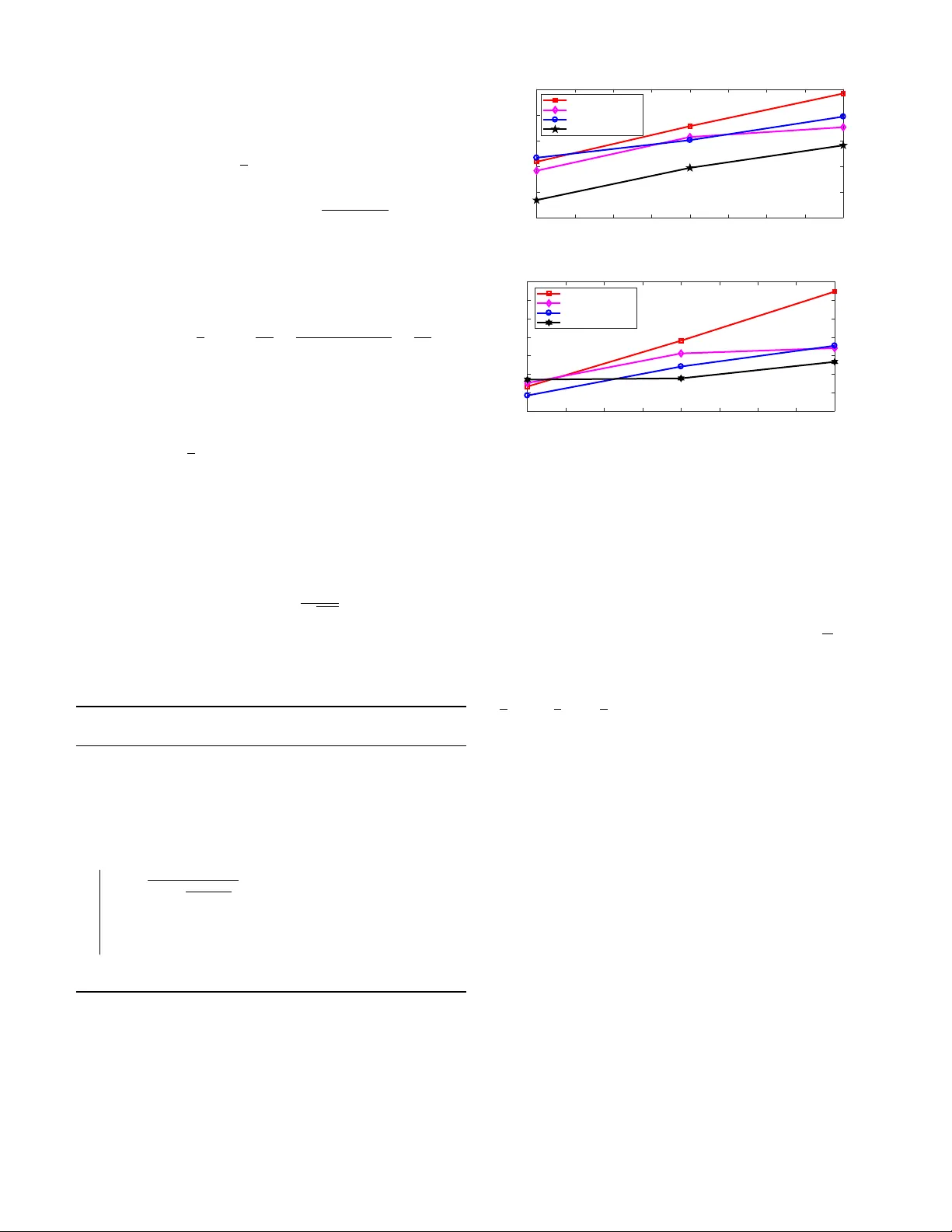
1 Multi v ariate Copula Spatial Dependenc y in One Bit Compressed Sensing Zahra Sadeghigol, Hadi Zayyani, Hamidreza Abin, and F arrokh Marv asti, Senior Member , IEEE Abstract —In this letter , the problem of sparse signal recon- struction from one bit compr essed sensing measurements is in vestigated. T o solve the pr oblem, a variational Bayes framework with a new statistical multivariate model is used. The dependency of the wa velet decomposition coefficients is modeled with a multivariate Gaussian copula. This model can separate marginal structure of coefficients from their intra scale dependency . In particular , the drawable Gaussian vine copula multivariate double Lomax model is suggested. The reconstructed signal is derived by variational Bay es algorithm which can calculate closed forms for posterior of all unknown parameters and sparse signal. Numerical r esults illustrate the effectiveness of the proposed model and algorithm compared with the competing appr oaches in the literature. Index T erms —one bit compressed sensing, vine copula model, variational Bayes. I . I N T RO D U C T I O N T HE extreme case of quantized Compressed Sensing (CS) [1]–[3] which is One bit Compressed Sensing (1b-CS) has enticed consideration newly [4]–[15]. This quantization procedure can achiev e greatly cost-effecti ve impact on the hardware. Traditional CS theory can reconstruct a sparse signal from much smaller number of linear measurements than the Nyquist rate [10], [11]. According to the CS paradigm, the procedure of quantization is omitted and assumed that the measurements are real. Ho wever , in the quantized CS, some discrete le vels are assigned to the measurements. In 1b-CS frame work, only tw o le vels are used to represent the measurements [4]- [15]. It is proved that only utilizing the sign of the measurements is sufficient to accurately reconstruct the sparse signal [3]. There are numerous algorithms suggested for the signal re- cov ery in 1b-CS framew ork [3]. In [4], an ` 1 -norm minimiza- tion is proposed which is known as Renormalized Fixed-Point Iteration (RFPI) algorithm. Authors in [5] presented Matching Sign Pursuit (MSP) algorithm for solving the problem. In [7], a Binary Iterativ e Hard Thresholding (BIHT) algorithm is appeared which is reported due to better accuracy than MSP . Furthermore, [6] introduced a Restricted-Step Shrinkage (RSS) method which is proved to hav e a guaranteed con ver gence. In [8], authors dev eloped an Adapti ve Outlier Pursuit (A OP) algorithm in the noisy 1b-CS scenario in which sign flip errors may exist. Also, a con ve x optimization solution is introduced in [9] to solve the problem. Moreov er, in [12] a V ariational Z. Sadeghigol is with the Department of Electrical Engineering, Sharif Univ ersity of T echnology , T ehran, Iran (e-mail: sadeghigol@gmail.com). H. Zayyani is with the faculty of Electrical and Computer Engineering, Qom Univ ersity of T echnology (QUT), Qom, Iran (e-mail: zayyani@qut.ac.ir). H. Abin and F . Marvasti are with the Department of Electrical Engineering, Sharif University of T echnology and Advance Communication Research Institute (A CRI), T ehran, Iran (e-mails: Hamidreza.abin@gmail.com; mar- vasti@sharif.edu). This work is fully supported by Iran National Science Foundation (INSF). Bayes (VB) algorithm is used for 1b-CS, while in [13] a Maximum A Posteriori (MAP) approach is presented for the signal recovery . In addition, a dictionary learning-based blind 1b-CS algorithm is suggested in [15]. Recently , authors in [16] rev ealed a new training-free 1b-CS approach for wireless neural recording. All the above algorithms are based on uni variate models causing to simple solutions. Nevertheless, these univ ariate models are not capable to describe statistical manner of wa velet coefficients completely . These simple models ignore an important stochastic property of wav elet coefficients which is the intrascale dependency across the same subband. T o ov ercome this problem, in this paper , a multiv ariate model is proposed which is based on copula distribution. In the best of our knowledge, multiv ariate models have not been considered in 1b-CS, yet. Howe ver , in the field of image processing, some researchers hav e tried to model the joint dependency of wa velet coefficients. Multi v ariate Gaussian distribution [17], Multiv ariate Generalized Gaussian Distribution (MGGD) [18] and Elliptically Contoured Distribution [19] have been pro- posed so far . The non-Gaussian joint stochastic manner of wa velet coef ficients can be demonstrated by Gaussian Scale Mixture (GSM) model [20], [21] and [22]. Some studies have recently worked on copulas for modeling multiv ariate wa velet coef ficients [23]–[25]. None of them considered the 1b-CS problem. The major advantage of copula is its flexibility for choosing v arious kinds of mar ginal distribu- tions based on the joint model. Accordingly , our contribution is as follows: 1) A new multiv ariate model which is named Drawable Gaussian V ine Copula-based Multiv ariate Double Lo- max (DGVC-MDL) is proposed for capturing the spatial intrascale dependencies of wav elet coefficients. 2) Based on this ne w proposed model, the full posteriors of unknown variables using VB are deriv ed in closed form. Simulation results demonstrate that the proposed DGVC- MDL improv es recovery performance in comparison to state of the art methods in the 1b-CS literature. The outline of the paper is as follows. Section II introduces the problem formulation. Then, the multiv ariate model is presented in Section III. The proposed variational inference procedure is illustrated in IV. Simulation results are presented in Section V. Finally , conclusions are drawn in Section VI. I I . P RO B L E M F O R M U L A T I O N The problem of sparse signal recovery from 1b-CS mea- surements can be formulated as follows: t = sign ( y ) = sign( Ax + w ) , (1) 2 Fig. 1. Diagonal dependency in the vine copula root trees. where A ∈ R n × m is the measurement matrix, t ∈ R n is the sign measurement vector of y ∈ R n , and n ∈ R n is the noise measurement vector which is assumed to be i.i.d random Gaussian with zero mean and variance σ 2 n . Our aim is to estimate the sparse signal x ∈ R m from the sign of measurements t . I I I . M U L T I V A R I A T E S TA T I S T I C A L M O D E L A. Basics The coefficients intrascale dependencies across subband are extensi vely considered before [23]. [26] has studied the amount of intraband and interband coef ficients dependency using mutual information. In the image denosing field, [19] and [21] introduced sev eral types of wa velet neighborhood. All these researches mentioned that the ov ercoming coefficients dependency is based on the intraband spatial structure. Using Chi-plot graphs, [23] demonstrated that the intraband depen- dency is more important than interorientation and interscale ones. Therefore, in this letter , we assume the intrascale depen- dency and ignore other kind of dependencies [23]. T o capture this dependency , the proposed algorithm introduces DGVC model which can provide an excellent marginal distribution fitting. Based on wa velet decomposition, scales and orientations subbands are formed. Three kinds of dependencies using DGVC are defined in the proposed algorithm as row depen- dency , column dependency and diagonal dependency . These three dependencies are modeled by vine copula trees across each row , column and diagonal, respecti vely . Because of large number of wa velet coef ficients, DGVC model is imposed in the proposed DGVC-MDL algorithm to capture the intrascale dependencies in ro w , column and diagonal directions. The diagonal tree of DGVC is depicted in Fig. 1. In this model, each node of the tree has a degree of at most 2, where the degree of a node indicates as the number of connections [27]. B. Multivariate Model Based on DGVC In this subsection, the proposed algorithm based on DGVC is introduced. A copula demonstrates a multiv ariate distribution with standard uniform marginal distributions [27]. The coefficients dependency is completely defined by the copula which is totally independent of the marginal distribution definition. A copula C can be considered as joint Cumulativ e Distribu- tion Function (CDF) on [0 , 1] d . Suppose a multiv ariate random variable ~ X = [ x 1 , ..., x d ] T with mar ginal CDFs F 1 , ..., F d . Sklar’ s theorem [28] expresses that a unique copula can be found such that: F ( x 1 , ..., x d ) = C ( F 1 ( x 1 ) , ..., F d ( x d )) . (2) The joint Probability Density Function (PDF) of ~ X can be written as: f ( x 1 , ..., x d ) = " d Y k =1 f k ( x k ) # × c ( F 1 ( x 1 ) , ..., F d ( x d )) , (3) where f k , k = 1 , ..., d are the marginal PDFs. W e consider the Gaussian copula in our proposed algorithm since it completely fits the statistical wavelet coefficient fea- tures. Besides the parameters of multiv ariate model base on Gaussian copula can be quickly estimated in the closed form by Maximum Likelihood (ML) method. The Gaussian copula density can be deriv ed from (2) as follows: c ( u 1 , ..., u d ) = 1 | Σ | 1 / 2 exp − ~ v ( | Σ | − 1 − I ) ~ v 2 , (4) where u i is uniform on [0 , 1] , ~ v = ( v 1 , ..., v d ) is a vector of transformed observations as v i = φ − 1 ( u i ) , and φ stands for the standard Gaussian CDF . I denotes an identity matrix with d × d dimension and Σ is the covariance matrix of ~ v . Multiv ariate copulas in higher dimensions are not proper and have some restrictions. Therefore, a fle xible model of copula is essential for capturing the high dimensional depen- dencies. [29] introduced regular vine copula and [30] presented it in detail. W e utilize DGVC in the proposed algorithm which its density is giv en by: f ( x 1 , ..., x d ) = " d Y k =1 f k ( x k ) # ×   d − 1 Y j =1 d − j Y i =1 c i,i + j | i +1 ,...,i + j − 1   , (5) where c i,j | i 1 ,...,i k := c i,j | i 1 ,...,i k ( F ( x i | x i 1 , ..., x i k ) , F ( x j | x i 1 , ..., x i k )) , (6) c j ( e ) ,k ( e ) | D ( e ) is a biv ariate copula density in a DGVC tree with the node set N := N 1 , ..., N d − 1 and the edge set E := E 1 , ..., E d − 1 . Each edge e = j ( e ) , k ( e ) | D ( e ) in E i represents by c j ( e ) ,k ( e ) | D ( e ) . j ( e ) and k ( e ) are nominated as the conditioned nodes and D ( e ) is called as the conditioning set [30]. More details in this regard can be found in [30]. C. Multivariate DGVC Modeling Estimation Suppose that ζ = ( ζ 1 , ..., ζ d ) and Σ represent the marginal PDF parameters and the copula cov ariance matrix, respec- tiv ely . Multiv ariate GVC hyperparameters are θ = ( ζ , Σ) which should be estimated. [31] represented that the copula covariance matrix ˆ Σ can be e valuated separately from the mar ginal PDF parameters ˆ ζ = ( ˆ ζ 1 , ..., ˆ ζ d ) . This assumption simplifies the estimation mechanism of hyperparameters as follows: 1) ˆ ζ = ( ˆ ζ 1 , ..., ˆ ζ d ) can be estimated using VB inference which will be described in the next section. 3 2) Utilizing the ML estimator , ˆ Σ can be e valuated in the following procedure. ML estimator for ˆ Σ : At each scale of wavelet decom- position, all coef ficients x should be transformed to v = φ − 1 ( F ( x | ζ )) . The transformed coef ficients are restructured into a matrix H = [ ~ V 1 , ..., ~ V M s ] and M s is the number of wa velet coefficients in scale s . ~ V i is a vector which contains a reference coefficient and its neighbors. It can be denoted as ~ V i = [ v i, 1 ...v i,L ] T and L is the neighborhood size. Therefore, Σ can be estimated using ML algorithm which leads to the sample covariance matrix of ~ V 1 , ..., ~ V M s : ˆ Σ = 1 M s M s X i =1 ~ V i ~ V T i = 1 M s H H T . (7) One of the rich distribution to represent the mar ginal manner of wav elet coefficients is Double Lomax (DL) PDF which is used in our proposed DGVC-MDL model. ML estimator f or ˆ η and ˆ f : T o ev aluate H in (7), param- eters of DL distrib ution should be computed which is gi ven by: n ˆ η , ˆ f o = argmax log η ,f M s Y i =1 f ( − → x i | η , f ) , (8) where f is DL PDF as following [32]: f ( x | η , f ) = η 2  1 + η | x | f  − ( f +1) , (9) with η > 0 as the scale parameter and f > 0 as the shape parameter [33]. ˆ η can be estimated by: ˆ η = M s P M s i =1 ( ( ˆ f +1) | x i | ˆ f + ˆ η | x i | ) , (10) ˆ f can be ev aluated using the numerical Newton-Raphson iterativ e procedure. D. Multivariate Double Lomax Model Based on Gaussian V ine Copula The proposed DGVC-MDL model is defined by f DGVC-MDL ( ~ x | θ ) =  η 2  d  1 + η | x | f  − d ( f +1) ×   d − 1 Y j =1 d − j Y i =1 c i,i + j | i +1 ,...,i + j − 1   . (11) The hyperparameters set is θ = ( η, f , Σ ) and d is the neighborhood size. The cov ariance matrix of ~ V is Σ using V i = φ − 1 ( F ( x i | η , f )) which φ denotes the standard normal CDF and F ( t | η , f ) = 1 2 ( sgn ( t ) + 1)  1 − 1 2  η t f + 1  − f  − 1 4 ( sgn ( t ) − 1)  1 − η t f  − f is the CDF of DL distribution. In order to impose VB on the proposed DGVC-MDL prob- abilistic model in (11), we ha ve to consider the hierarchical form of DL distribution which is introduced by: p ( x | τ ) = n Y i =1 p ( x i | τ i ) = n Y i =1 N ( x i | 0 , τ i ) , (12) p ( τ | λ ) = n Y i =1 E xp ( τ i | λ 2 2 ) , (13) p ( λ ) = n Y i =1 G amma ( λ i | f , f ) , (14) where τ and λ are the precision of Gaussian PDF and exponential PDF parameter , respectively . I V . P RO P O S E D V A R I A T I O N A L I N F E R E N C E P R OC E D U R E T o deri ve the posterior PDF of unkno wn v ariables, VB inference is imposed in the proposed algorithm. Suppose Ψ , { x, τ , λ } is assigned to all v ariables in our proposed model. T o model the sign function in (1), we use the deriv ation of [12]. An approximation of the posterior PDF p ( Ψ | t ) can be obtained by maximizing L ( q ) = Z q ( Ψ ) ln p ( t , Ψ ) q ( Ψ ) d Ψ , (15) where p ( t , Ψ ) is stated as p ( t , Ψ ) = p ( t | x ) p ( x | τ ) p ( τ | λ ) p ( copula ) , (16) p ( copula ) is the second part of (5). p ( t | x ) in (16) is difficult to ev aluate. T o overcome this problem, [12] found a lower bound on L ( q ) using the following inequality σ ( y ) t [1 − σ ( y )] 1 − t = σ ( z ) ≥ σ ( δ ) exp  z − δ 2 − λ ( δ )( z 2 − δ 2 )  , (17) where z = (2 t − 1) y , λ ( δ ) = (1 / 4 δ ) tanh δ / 2) , tanh( x ) is stated to the hyperbolic tangent function which is tanh( x ) , (exp( x ) − exp( − x )) / (exp( x ) + exp( − x )) . The equality is achiev ed when δ = z . Utilizing equation (17), [12] obtained p ( t | x ) ≥ F ( t , x , δ ) , n Y i =1 σ ( δ i ) exp  z i − δ i 2 − λ ( δ i )( z 2 i − δ 2 i )  . (18) Then [12] defined G ( t , Ψ , δ ) , F ( t , x , δ ) p ( x | τ ) p ( τ | λ ) p ( copula ) to compute a lower bound on L ( q ) . The different steps of VB procedure are represented as follows. 1. Update of q x ( x ) : The variational approximation of the posterior PDF q x ( x ) can be deriv ed by ln q x ( x ) ∝ h ln F ( t , x , δ ) + ln p ( x | τ ) + ln p ( copula ) i τ ∝ * n X i =1  z i 2 − λ ( δ i ) z 2 i  − x 2 2 τ − v T (Σ − 1 v − I ) v 2 + τ , n ∝ − x T A T Λ δ Ax + 1 2 (2 t − 1) T Ax − 1 2  x T Λ τ x  τ − v T (Σ − 1 v − I ) v 2 , (19) where Λ τ , diag ( τ 1 , ..., τ m ) and [12] denoted that Λ δ , diag ( λ ( δ 1 ) , ..., λ ( δ n )) . h·i ev aluates expectation with respect to a random variable. 4 Obviously q x ( x ) has a Gaussian posterior PDF with the following parameters: µ x = Σ x A T  1 2 (2 t − 1) − 2Λ δ µ n  , (20) Σ x =  Λ h τ i + 2 A T Λ δ A + (Σ − 1 v − I ) τ  − 1 . (21) The third part of (21) captures the dependency of wav elet coefficients using proposed copula model. 2. Update of q τ ( τ ) : The posterior PDF of q τ ( τ ) can be deriv ed by ln q τ ( τ ) ∝  − 1 2 ln τ − x 2 2 τ − v T (Σ − 1 v − I ) v 2 − λ 2 2 τ  x , λ , (22) where τ has the Generalized In verse Gaussian (GIG) distribu- tion with the following parameters: τ ∼ GIG  1 2 , h x 2 i + x T (Σ − 1 v − I ) x , h λ 2 i  . (23) 3. Update of q λ ( λ ) : In the same way , variational approxima- tion of yields ln q λ ( λ ) ∝ h ln p ( τ | λ ) + ln p ( λ ) i τ . (24) By setting f = 0 , the posterior PDF of λ becomes Rayleigh distribution. λ ∼ Rayleigh ( λ | 1 p h τ i ) . (25) The posterior PDF of n , β and δ can be found in [12]. The ov erall 1b-CS recovery based on DGVC-MDL algorithm is summarized in Algorithm 1. Algorithm 1: The proposed DGVC-MDL algorithm for 1b-CS recovery input : Array output t ∈ R n × 1 based on model (1) Measurement matrix A ∈ R n × m output: wa velet coefficients estimation x ∈ R m Initialize τ , λ and δ while iter < maxiter do ˆ η = M s P M s i =1 ( ( ˆ f +1) | x i | ˆ f + ˆ η | x i | ) ; update µ x and Σ x using (20) and (21); update τ using (22); update λ using (25); end b x ← µ x / norm( µ x ) ; V . S I M U L A T I O N R E S U LT S The performance of the proposed DGVC-MDL algorithm is inv estigated in this section. The measurement matrix A ∈ R n × m is randomly drawn from N (0 , 1) with i.i.d entries and A ’ s columns are normalized to unit value. Our proposed algorithm is compared with the BIHT algorithm [7], the 1- BCS, R1-BCS [12] and A OP [8]. Note that the BIHT algorithm 2 2.5 3 3.5 4 4.5 5 5.5 6 Sampling Rate 8 10 12 14 16 18 SNR Proposed DGVC-MDL R1-BCS 1-BCS AOP (a) Baboon-SNR 2 2.5 3 3.5 4 4.5 5 5.5 6 Sampling Rate 11 12 13 14 15 16 17 18 SNR Proposed DGVC-MDL R1-BCS 1-BCS AOP (b) SAR-SNR Fig. 2. SNR versus sampling rate. has been also simulated. Howev er, due to the small SNR of this method, the corresponding results are not represented here. The SNR is utilized to demonstrate the performance of the proposed DGVC-MDL algorithm over 10 2 independent runs. Fig. 3 illustrates the reconstruction SNR versus the sampling rate where the initial values of τ , λ and δ are 10 − 8 , 10 − 8 and 1 , respectiv ely . The sampling rate which equals n m is the ov ersampling ratio; it varies from 2 to 6 . W e set m = 1024 for input image of size 32 × 32 and we consider the wa velet coefficients at the second decomposition of the SAR image e2 981006 18093 2889 1 and Baboon. When the sampling rate equals 2, the SNR is near to R1-BCS and 1-BCS, howe ver when the sampling rate increases the SNR improves up to 2.5 dB compared to R1-BCS, one-BCS and A OP . V I . C O N C L U S I O N In this paper, a new statistical model based on copula distribution is proposed for 1b-CS to capture the intrascale dependencies between wa velet coef ficients. The VB of this new model is deri ved mathematically and it can estimate all unknown parameters in closed forms. The reconstruction SNR of the proposed algorithm is 2.5 dB better than SNR of other methods when the sampling rate is equal to 6. 1 The test image is chosen from the Coastal En vironmental Assess- ment Regional Activity Centre (CEARA C) database which can be found in http://cearac.poi.dvo.ru/en/db/ 5 R E F E R E N C E S [1] A. Zymnis, S. Boyd, and E. Candes, “Compressed sensing with quan- tized measurements, ” IEEE Signal Processing Letters , vol. 17, no. 2, pp. 149–152, 2010. [2] A. Moshtaghpour , L. Jacques, V . Cambareri, K. Degraux, and C. De Vleeschouwer , “Consistent basis pursuit for signal and matrix estimates in quantized compressed sensing, ” IEEE Signal Pr ocessing Letters , vol. 23, no. 1, pp. 25–29, 2016. [3] H. Zamani, H. Zayyani, and F . Marvasti, “ An iterativ e dictionary learning-based algorithm for doa estimation, ” IEEE Communications Letters , vol. 20, no. 9, pp. 1784–1787, 2016. [4] P . T . Boufounos and R. G. Baraniuk, “1-bit compressive sensing, ” in Information Sciences and Systems, 2008. CISS 2008. 42nd Annual Confer ence on . IEEE, 2008, pp. 16–21. [5] P . T . Boufounos, “Greedy sparse signal reconstruction from sign measurements, ” in Signals, Systems and Computers, 2009 Conference Recor d of the F orty-Third Asilomar Conference on . IEEE, 2009, pp. 1305–1309. [6] J. N. Laska, Z. W en, W . Y in, and R. G. Baraniuk, “Trust, b ut verify: Fast and accurate signal recovery from 1-bit compressi ve measurements, ” IEEE Tr ansactions on Signal Processing , vol. 59, no. 11, pp. 5289– 5301, 2011. [7] L. Jacques, J. N. Laska, P . T . Boufounos, and R. G. Baraniuk, “Robust 1- bit compressive sensing via binary stable embeddings of sparse vectors, ” IEEE T ransactions on Information Theory , vol. 59, no. 4, pp. 2082– 2102, 2013. [8] M. Y an, Y . Y ang, and S. Osher, “Robust 1-bit compressi ve sensing using adaptive outlier pursuit, ” IEEE T ransactions on Signal Processing , vol. 60, no. 7, pp. 3868–3875, 2012. [9] Y . Plan and R. V ershynin, “Robust 1-bit compressed sensing and sparse logistic regression: A con vex programming approach, ” IEEE T ransactions on Information Theory , vol. 59, no. 1, pp. 482–494, 2013. [10] E. J. Candes and T . T ao, “Near-optimal signal recovery from random projections: Universal encoding strategies?” IEEE transactions on infor- mation theory , vol. 52, no. 12, pp. 5406–5425, 2006. [11] D. L. Donoho, “Compressed sensing, ” IEEE T ransactions on information theory , vol. 52, no. 4, pp. 1289–1306, 2006. [12] F . Li, J. F ang, H. Li, and L. Huang, “Robust one-bit bayesian compressed sensing with sign-flip errors, ” IEEE Signal Processing Letters , vol. 22, no. 7, pp. 857–861, 2015. [13] X. Dong and Y . Zhang, “ A map approach for 1-bit compressive sensing in synthetic aperture radar imaging, ” IEEE Geoscience and Remote Sensing Letters , vol. 12, no. 6, pp. 1237–1241, 2015. [14] W . Chen, I. J. W assell, and M. R. Rodrigues, “Dictionary design for distributed compressiv e sensing, ” IEEE Signal Processing Letters , vol. 22, no. 1, pp. 95–99, 2015. [15] H. Zayyani, M. Korki, and F . Marvasti, “Dictionary learning for blind one bit compressed sensing, ” IEEE Signal Processing Letters , vol. 23, no. 2, pp. 187–191, 2016. [16] B. Sun and Y . Ni, “ A training-free one-bit compressed sensing frame- work for wireless neural recording, ” IEEE Communications Letters , 2017. [17] G. Tzagkarakis, B. Beferull-Lozano, and P . Tsakalides, “Rotation- in variant texture retrieval with gaussianized steerable pyramids, ” IEEE T ransactions on Image Processing , vol. 15, no. 9, pp. 2702–2718, 2006. [18] D. Cho and T . D. Bui, “Multiv ariate statistical modeling for image denoising using wavelet transforms, ” Signal Processing: Image Com- munication , vol. 20, no. 1, pp. 77–89, 2005. [19] S. T an and L. Jiao, “Multiv ariate statistical models for image denoising in the wav elet domain, ” International Journal of Computer V ision , vol. 75, no. 2, pp. 209–230, 2007. [20] M. J. W ainwright and E. P . Simoncelli, “Scale mixtures of gaussians and the statistics of natural images, ” in Advances in neural information pr ocessing systems , 2000, pp. 855–861. [21] J. Portilla, V . Strela, M. J. W ainwright, and E. P . Simoncelli, “Image denoising using scale mixtures of gaussians in the wav elet domain, ” IEEE T ransactions on Image pr ocessing , vol. 12, no. 11, pp. 1338–1351, 2003. [22] L. Boubchir, A. Nait-Ali, and E. Petit, “Multivariate statistical modeling of images in sparse multiscale transforms domain, ” in Image Pr ocessing (ICIP), 2010 17th IEEE International Confer ence on . IEEE, 2010, pp. 1877–1880. [23] N.-E. Lasmar and Y . Berthoumieu, “Gaussian copula multivariate modeling for texture image retriev al using wavelet transforms, ” IEEE T ransactions on Image Processing , vol. 23, no. 5, pp. 2246–2261, 2014. [24] R. Kwitt, P . Meerwald, and A. Uhl, “Efficient texture image retrieval using copulas in a bayesian framework, ” IEEE transactions on image pr ocessing , vol. 20, no. 7, pp. 2063–2077, 2011. [25] Y . Stitou, N. Lasmar , and Y . Berthoumieu, “Copulas based multiv ariate gamma modeling for texture classification, ” in Acoustics, Speech and Signal Pr ocessing, 2009. ICASSP 2009. IEEE International Confer ence on . IEEE, 2009, pp. 1045–1048. [26] D.-Y . Po and M. N. Do, “Directional multiscale modeling of images using the contourlet transform, ” IEEE Tr ansactions on image pr ocessing , vol. 15, no. 6, pp. 1610–1620, 2006. [27] E. C. Brechmann, C. Czado, and K. Aas, “Truncated regular vines in high dimensions with application to financial data, ” Canadian Journal of Statistics , vol. 40, no. 1, pp. 68–85, 2012. [28] A. Sklar, “Random variables, joint distribution functions, and copulas, ” K ybernetika , vol. 9, no. 6, pp. 449–460, 1973. [29] T . Bedford and R. M. Cooke, “V ines: A new graphical model for dependent random variables, ” Annals of Statistics , pp. 1031–1068, 2002. [30] D. Kurowicka and R. M. Cooke, Uncertainty analysis with high dimen- sional dependence modelling . John Wiley & Sons, 2006. [31] H. Joe and J. J. Xu, “The estimation method of inference functions for margins for multivariate models, ” 1996. [32] X. Gu, H. Leung, and X. Gu, “ A variational bayesian approach to compressiv e sensing based on double lomax priors, ” in Acoustics, Speech and Signal Processing (ICASSP), 2013 IEEE International Confer ence on . IEEE, 2013, pp. 5994–5998. [33] C. Kleiber and S. Kotz, Statistical size distributions in economics and actuarial sciences . John Wiley & Sons, 2003, vol. 470.