Sensor Selection and Random Field Reconstruction for Robust and Cost-effective Heterogeneous Weather Sensor Networks for the Developing World

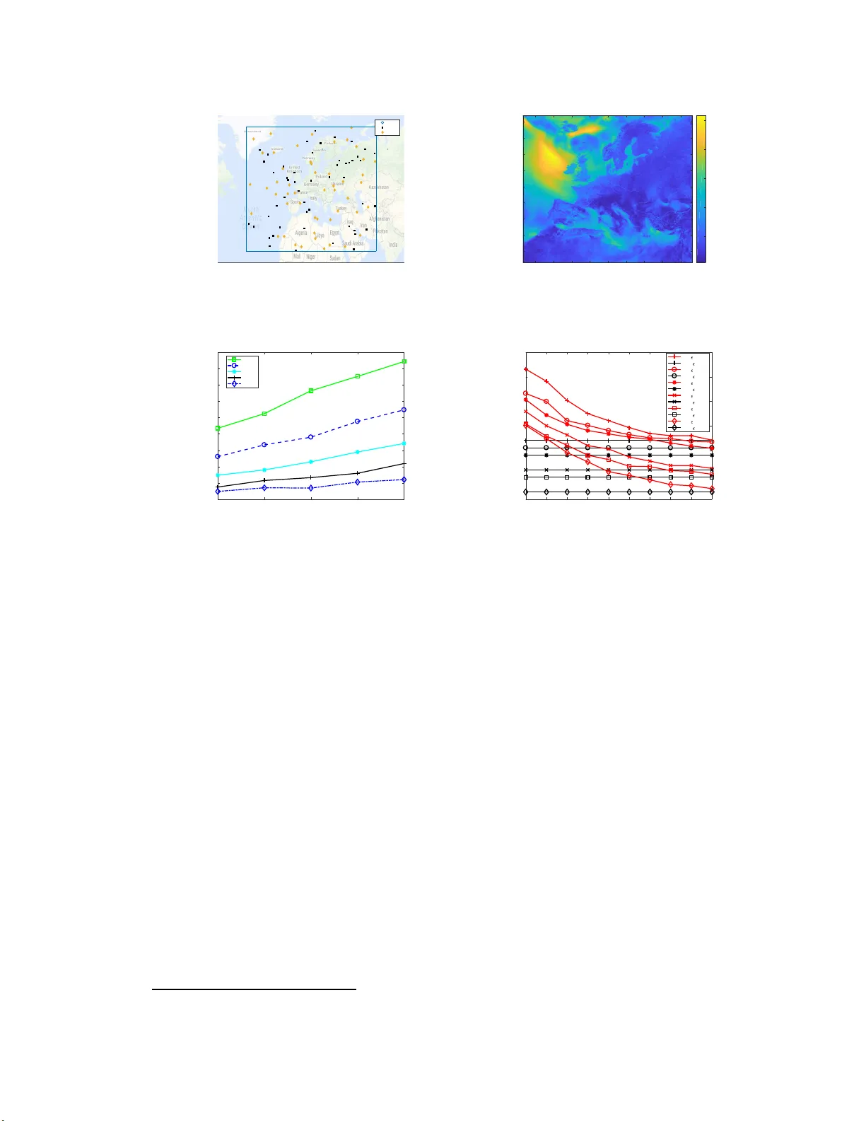
Sensor Selection and Random Field Reconst ruction for Robust and Cost-effective Heteroge neous W eather Senso r Networks for the Developi ng W orld Pengfei Zhang University of Oxford Oxford, UK Ido Nevat TUM CREA TE Singapore Gareth W . Peters Heriot-W att University Scotland, UK W olfgan g Fruehwirt University of Oxford Oxford, UK Y ongcha o Huang University of Oxford Oxford, UK Ivonne Ande rs ZAMG V ienna, Austria Michael Osborne University of Oxford Oxford, UK Abstract W e address the tw o fundamental problems of spatial field reconstruction a nd sensor selection in heterogeneous sensor networks: (i) how to efficiently per- form spatial field r econstruction based on measurements obtained simulta- neously from networks with both high and low quality sensors; a nd (ii) how to perform query based sensor set selection with predictive MSE p erfor- mance guarantee . For the first problem, we developed a low complexity algorithm based on the sp atial best linear unbiased estimator (S-BLU E ). Next, building on the S-B LUE, we address the second problem, and develop an efficient algorithm for query based sensor set selection with p erformance guar- antee . Our algorithm is ba sed on the Cross Entropy method wh ich solves the combinatorial optimization pr oblem in an efficient manner . 1 Introduction W e con sider the case where two types of sensors are de p loyed: the first consis ts of expen- sive, high quality sensors; and the second, of cheap low quality sensors, which are activated only if the intensity of the spa tial field exceed s a pre-defined activation threshold (eg. wind sensors). This type of heterogeneous sensor networks approach has gained a ttention in the last few yea rs due to the vision of the Internet of Things (IoT) where networks may share their data over the internet [1, 2]. T wo practical scenarios 1 that are of importance are: firstly , high-quality sensors may be deployed by government agencies (eg. weather stations). These are sparsely deployed due 1 In particular , developing world countries are constrained by their budget when purchasing equipment. Meanwhile, these countries are heavily effected by climate change. T his combination makes the robust and cost-effective sensor sele ction i n weather sensor networks a major concern for the developing world. 31st Conference on Neural Information Processing Systems (NIPS 2017), Lo ng Beach, CA, USA. to their high costs, limited space constraints, high power consumption etc. T o improve the coverage of the WSN, low-quality cheap sensors ca n be deployed to augment the high- quality sensor network [3]; Secondly , High-quality sensors cannot be ea sily deployed in remote locations, for example in ocea ns, lakes, mountains and volcanoes. In these cases, battery oper ated low-quality chea p sensors ca n be de p loyed [4]. More specifically , the followin g two funda mental problems are the focus of this paper: Firstly , Spatial fi e ld reconstruction : the task is to accur a tely estimate and predict the inten- sity of a spa tial random field, not only at the locations of the sensors, b ut at a ll locations [5– 7], given heterogeneous observations from both sensor networks; Secondly , Query based sensor set selection with performance guarantee : the task is to perform on-line sensor set selection which meets the QoS cr iter ion imposed by the user , as well as minimises the costs of activating the sensors of these networks [8 – 1 0]. 2 System model W e now present the system model for the physical phenomenon observed by two types of networks. A1 Cons ider a random spatial phenomenon (eg. wind) to be monitored defined over a 2 - dimensional space X ∈ R 2 . The mea n response of the physical process is a smooth contin uous spatial function f ( · ) : X 7→ R , and is modelled as a Gaussi an Process (GP) according to f ( x ) ∼ G P ( µ f ( x ; θ f ) , C f ( x 1 , x 2 ; Ψ f )) , (1) where the mean and covariance functions µ f ( x ; θ f ) , C f ( x 1 , x 2 ; Ψ f ) are assumed to be known. A2 Let N be the total number of sensors that are deployed over a 2 -D region X ⊆ R 2 , with x n ∈ X , n = { 1 , · · · , N } being the physical location of the n -th sensor , assumed known by the FC. The number of sensors d eployed by Network 1 a nd Network 2 a re N H and N L , respectively , so that N = N H + N L . A3 Sensor network 1 incl udes hi gh qu ality se nsors. T he sensors have a 0 -threshold activation and each of the sensors collects a noisy observation of the spatial phe- nomenon f ( · ) . At the n -th sensor , located at x n , the observa tion is given by: Y H ( x n ) = f ( x n ) + W ( x n ) , n = { 1 , · · · , N H } (2) where W ( x n ) is i.i.d Gaussian noise W ( x n ) ∼ N  0 , σ 2 W  . Sensor network 2 in- cludes low quality sen sors. The sensors have a T -threshold activation and e a ch of the sensors collects a noisy observation of the spatial phenomenon f ( · ) , only if the intensity of the field at that location exceed s the pre-defined threshold T , (eg. anemometer sensors for wind monito ring [11, 12]). At the n - th sensor , located at x n , the observa tion is given by: Y L ( x n ) =  f ( x n ) + V ( x n ) , f ( x n ) ≥ T V ( x n ) , f ( x n ) < T (3) where V ( x n ) is i.i.d Gaussian noise V ( x n ) ∼ N  0 , σ 2 V  . 3 Field Reconstruction via Spatial Best Linear Unbiased Estimator (S-BLUE) T o perform inference in our Ba yesian framework, one would typically be interested in com- puting the predictive posterior density at any location in space, x ∗ ∈ X , denoted p ( f ∗ | Y N ) . Based on this quantity , a point estimator , like the Minimum M ean Squared Error ( M MSE) estimator can be d erived: b f ∗ MMSE = ∞ Z −∞ p ( f ∗ | Y N , x 1:N , x ∗ ) f ∗ d f ∗ W e develop the spatial field reconstr uction via Best L inea r Unbiased Estimator (S- BLUE), which enjoys a low computational complexity [13]. The S-BLUE d oes not requir e ca lculat- ing the predictive posterior density , but only the first two cross moments of the model. The S-BLUE is the optimal (in terms of minimizing Me an Squared Error (MSE)) of all linear estimators a nd is given by the solution to the following optimization problem: b f ∗ := b a + b BY N = arg min a, B E h ( f ∗ − ( a + BY N )) 2 i , (4) where b a ∈ R and b B ∈ R 1 × N . The optimal linea r estimator that solves (4) is given by ˆ f ∗ = E f ∗ Y N [ f ∗ Y N ] E Y N [ Y N Y N ] − 1 ( Y N − E [ Y N ]) , (5) and the M ean S quared Error (MS E) is given by σ 2 ∗ = k ( x ∗ , x ∗ ) − E f ∗ Y N [ f ∗ Y N ] E Y N [ Y N Y N ] − 1 E Y N f ∗ [ Y N f ∗ ] . (6) 4 Query Based Sensor Set Selection with Performance Guarantee In this Section we de v e lop an algorithm to perform on-line sensor set selection in order to meet the requirements of a query mad e by users of the system. In this scenario users can prompt the system and request the system to provide an estimated value of the spatial random field at a location of interest x ∗ . W e defined the activation sets of the sensors in both networks by S 1 ∈ { 0 , 1 } | N H | , S 2 ∈ { 0 , 1 } | N L | . Then the sensor selection problem can be formulated as follows: S = arg min     S 1 ∈{ 0 , 1 } | N H | S 2 ∈{ 0 , 1 } | N L |     w h |S 1 | + w l |S 2 | , s.t. σ 2 ∗ < σ 2 q , (7) where σ 2 q is the maximal allowed uncertainty at the query location x ∗ , and w h and w l are the known c osts of ac tiva ting a sensor from Network 1 a nd Network 2 , respectively . Suppose we wish to maximize a function U ( x ) over som e set X . Let us denote the maxi- mum by γ ∗ ; thus, γ ∗ = ma x x ∈ X U ( x ) . (8) The Cross Entropy Method ( CEM) solves this optimization problem by casting the original problem (8) into an estimation problem of r are-event probabilities. By d oing so, the CEM aims to locate an optimal para metric sampling distribution, that is, a probability distribu- tion on X , rather than locating the optimal solution directly . T o ap p ly the CEM to solve our optimization problem in (7), we need to choose a par ametric d istribution. Since the ac- tivation of the sensors is a binary varia ble ( e g. 0 → don’t activa te , 1 → a c tivate), we choose an independent Bernoulli va riable as our parametric distribution, with a single para meter p (ie. V = p ). The Bernoulli distribution is a member of the NEF of distributions, hence, an analytical solution of the stochastic program is availa b le in closed form as follows: p t,j = K P i =1 1  Γ H i , j = 1  1 ( U ( k ) ≥ β t ) K P i =1 1 ( U ( k ) ≥ β t ) . Since the optimization problem in Eq. (7) is a constrained optimization problem, we in- troduce an Accept \ Reject step which rejects samples which do not meet the QoS criterion σ 2 ∗ < σ 2 q , as f ollows U ( k ) =  −  w h   S H   + w l   S L    , σ 2 ∗ ( k ) < ǫ −∞ , Otherwise -60 -40 -20 0 20 40 60 80 20 30 40 50 60 70 80 Region of interest High Low -50 -35 -20 -5 10 25 40 55 70 20 27 34 41 48 55 62 69 76 5 10 15 20 25 Figure 1 : Left pa nel: ma p of region of interest with sensors locations. Right panel: Storm wind intensity map 50 100 150 200 250 N l 0 1 2 3 4 5 6 7 8 9 MSE N=300 N=400 N=500 N=600 N=700 1 2 3 4 5 6 7 8 9 10 Number of Iterations 0 100 200 300 400 500 600 U CE = 3.4 Opt = 3.4 CE = 3.6 Opt = 3.6 CE = 3.8 Opt = 3.8 CE = 4 Opt = 4 CE = 4.2 Opt = 4.2 CE = 4.4 Opt = 4.4 Figure 2: Left panel: MSE with effect of differ ent number of high and low quality sensors. Right panel: Comparison of U values between optimal scheme and CE method with effect of number of itera tions. 5 Experimental Results and Discussion In order to test our algorithm on real d ata sets, we use fine gr a ined da tasets availa ble from Hans-Ertel-Centre f or W eather Research (HErZ) proj ect 2 . P articularly , we choose Feb 23, 2015 a s testing data since it has the highest wind speed across the whole year . The lef t panel of Fig. 1 shows the region of interest on the map. Both high and low quality sensors are selected randomly within the region. In this figure we randomly deployed 50 high quality and 5 0 low quality sensors. The right panel of Fig. 1 shows daily wind speed intensity a cross the region. In left panel of Fig. 2 we present a quantitative compar ison of the MSE for v a rious values of high and low quality sensors. The result shows a clea r trend of MSE with the increasing of high a nd low quality sensors. W e a lso illustrate how our sensor selection algorithm performs. For comparison, we use an optimal selection method which only selects the sensor set collection s that minimize the U values a nd ensures that the QoS criterion is being met. The simulation para meters we have are: { N h = 5 , N l = 10 , T = 0 , w h = 150 , w l = 30 , σ w = 0 . 00 1 , σ g = 0 . 003 , k f ( x ∗ , x ∗ ) = 5 . 8 , x ∗ = 10 , y ∗ = 50 , ǫ = { 3 . 4 , 3 . 6 , 3 . 8 , 4 , 4 . 2 , 4 . 4 }} . W e fix the N h = 5 , N l = 10 . The comparison is shown in right panel of Fig. 2. W e also incr ease the number of itera tions in CE method from 1 to 10 . It shows CE method converges quickly to the optimal selection algorithm within 10 iter a tions for all the ǫ values. References [1] Jayava rdhana Gubbi, Rajkumar Buyya, Slaven Marusic, and Marimuthu Palaniswa mi. Inter - net of Things ( IoT ): A vision, architectural elements, and future directions. Future Generation 2 https://www .herz-tb4.uni-bonn.de/index.php/hans-ertel-centre-for-weather- research/funding Computer Systems , 29(7):1645 –1660, 2013. [2] Ovidiu V ermesan, Pe ter Friess, Pat rick Guillemin, Sergi o Gusme roli , Harald Sundmaeker , Alessandro Bassi, Ignacio Soler Jubert, Margaretha Mazura, Mark Harrison, M Eisenhauer , and Others. Internet o f things strategic research roadmap. O. V ermesan, P . Friess, P . Guillemin , S. Gusmeroli, H. Sundmaeker , A. Bassi, et al., Intern et of Things: Global T echnological and Societal T rends , 1:9–52, 2011. [3] Sut harshan Rajasegarar , Peng Zhang, Y ang Zhou, Shanika Karunasekera, Christopher Le ckie, and Marimuthu Palaniswami. High resolution spatio-temporal monitoring of air pollutants using wireles s s ensor networks. In 2014 I EEE Nint h International Con ference on Intelligent Sensors, Sensor Networks and Information Processing (ISS NIP) , pages 1–6. IEEE, 2014. [4] Geoffr ey W erner-Allen, Konrad Lorincz, M ario Rui z, Omar Marcillo, Jeff Johnson, Jonathan Lees, and Matt W elsh. Deplo ying a wireless sensor network on an active volcano. IEEE Internet Computing , 10(2):18–25, 2006. [5] Gar eth W Pe ter s, Ido Nevat, and T omok o Matsui. How to Utilize Sensor Network D ata to Efficiently Per form Model Calibration and Spatial Field Reconstruction. In Modern Methodology and Applications in Spatial-T emporal Modeling , pages 25–62. Springer , 2015. [6] Ido Nevat, Gareth W Peters, F rancois Septier , and T omok o Matsui. Estimation of Spatially Cor- related Random Fields in Heterogeneous W ireless Sensor Networks. IEEE T ransactions on Signal Processing , 63(10):2597–260 9, 2015. [7] Ido Nevat, Gareth W Peters, and Iain B Coll ings. Random Fie ld Reconstruct ion W ith Quantiza - tion in W i rele ss Sensor Networks. IEEE T ransactions on Signal Proce ssing , 61:6020–6033 , 2013. [8] Miguel Calvo-F ullana, Javier Matamoros, and Carles Ant ´ on-Haro. Sensor Selection and Power All ocation Strategies for Energy Harvesting W ireles s Sensor Networks. arXiv pr eprint arXiv:1608.038 75 , 2016. [9] Siddharth Joshi and Stephen Boy d. Sensor s e lection via convex optimization. IE EE T ransactions on Signal Processing , 57(2):451–462, 2009. [10] Sundeep Prabhakar Chepuri and Geert Leus. Sparsity-promoting sensor se l ection for non-linear measurement mod e ls. IEE E T ransactions on Signal Proces sing , 63(3):684–69 8, 2015. [11] Anemometer W ind Speed Sensor w/Analog V oltage Output. T echnical report, 2015. [12] ANEM O 4403 RF WINDSPEED METER (ANEMOME TER) WITH WM44 P RF DISPLA Y UNIT WIRELESS WIND SPEED METER. T echnical report, 2015. [13] S M Kay . Fundamentals of Statistical Signal Pr ocessing, V olume 2: Detection Theory . Prentice Hall PTR, 1998.