Kullback-Leibler Principal Component for Tensors is not NP-hard

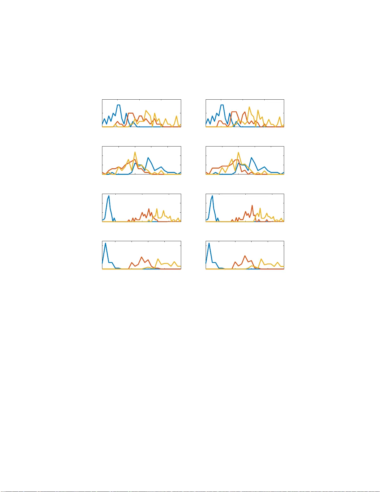
Kullback-Leibler Principal Componen t for T ensors is not NP-hard Ke jun Huang * Nicholas D. Sidiropoulo s † Abstract W e study the problem of nonn egati v e rank-one approximation of a nonne gativ e tensor , and sho w that the globally optimal solution that minimizes the generalized Kullback-Leibler di ver gence can be efficiently obtained, i.e., i t is not NP- hard. This result works f or arbitrary nonnegati v e tensors with an arbitrary number of modes (i ncluding two, i.e. , matrices). W e derive a closed-form expression for the KL principal component, which is easy to compute and has an intuitiv e proba- bilistic interpretation. For generalized KL approximation with higher ranks, the problem i s for the fi rst time sho wn to be equi v alent to multinomial latent v ariable modeling, and an iterative algorithm is derived that r esembles the expectation- maximization algorithm. On the Iris dataset, we sho wcase ho w the deri ved results help us learn t he model in an unsupervised manner , and obtain strikingly close performance to that from supervised methods. 1 Introd uction T ensors are powerful too ls for big data an alytics [1], ma in ly thanks to the a b ility to uniquely identify latent factors under mild condition s [2, 3]. On the other hand, most detection and estimation problem s related to tensors are NP-har d [ 4]. A similar situ- ation is encou ntered in n onnegative matrix factorization, which is essentially un ique under certain c o nditions [5, 6] and c omputatio n ally NP-hard [ 7]. In a lot of ap plica- tions, n o nnegativity constraints a r e natu r al for te n sor latent factors as well. In practice, th e la te n t factor s o f tensor s and matrices are usually ob tained b y min i- mizing the mismatch between the data and the factor iz a tion m odel according to ce rtain loss measures. The most pop ular loss measures the su m o f the element-wise squared errors, which is concep tually ap pealing and condu civ e for algorithm design, thank s to the success of least-squa res-based me thods. For exam ple, an effectiv e algorith m fo r minimizing the least-squares loss is A O-ADMM [8], an d we refer the readers to the referenc e s therein for othe r least-squares-based methods. From an estimation theoretic point of view , the least-squares loss admits a maxim um-likelihood in ter pretation under i.i.d. Gaussian noise. In a lot of applications, howe ver, it rem ains qu estionable whether Gaussian no ise is a suitable model for nonnegative data. * Uni ve rsity of Minnesota, Minneapoli s, MN 55455. Email: huang6 63@umn.edu † Uni ve rsity of V ir ginia , Charl ottesvi lle, V A 22904. Email: nikos@virginia.edu 1 W e study the proble m of fitting a non negativ e data matrix/tensor Y with low rank factors, using the gene ralized K ullback-L eibler (KL) div ergence as the fitting c riterion. Mathematically , given a N -way tensor data Y ∈ R J 1 × ... × J N and a target rank K , we try to fin d factor matrices constituting a canonical polyadic d ecompo sition (CPD) that best app roximates the data tensor Y in terms of generalized KL diver gence: minimize λ , { P ( n ) } X j 1 ,...,j N − Y j 1 ...j N log K X k =1 λ k N Y n =1 P ( n ) j n k + K X k =1 λ k N Y n =1 P ( n ) j n k ! subject to λ ≥ 0 , P ( n ) ≥ 0 , 1 ⊤ P ( n ) = 1 ⊤ , ∀ n ∈ [ N ] . (1) The condition s i mposed in Problem (1) besides nonnegativity are intend ed for resolving the trivial scaling amb iguity in herent in matrix factorizatio n and tensor CPD models, and thus are witho ut loss of gener a lity : the colum ns of all the factor matrices are no r- malized to sum up to on e , a n d the scalings are absorb ed into the correspond ing values in the vector λ . W e adopt the common nota tio n [ [ λ ; P ( 1 ) , ..., P ( N ) ] ] to denote the tensor synthesized fr om the CPD model using these factors. An instant advantage of this formulation is that the loss function of (1) ca n be greatly simplified . Thank s to the constraints 1 ⊤ P ( n ) = 1 ⊤ , it is easy to see that X j 1 ,...,j N K X k =1 λ k N Y n =1 P ( n ) j n k = K X k =1 λ k . Therefo re, Problem (1) is mathema tically equiv alent to minimize λ , { P ( n ) } − X j 1 ,...,j N Y j 1 ...j N log K X k =1 λ k N Y n =1 P ( n ) j n k + 1 ⊤ λ subject to λ ≥ 0 , P ( n ) ≥ 0 , 1 ⊤ P ( n ) = 1 ⊤ , ∀ n ∈ [ N ] . (2) 2 Motivation: Probabilistic Latent V ariable Modeling Most of the existing literature moti vates the use of g eneralized KL-div ergence by mod- eling the nonnegative integer data as generated from Poisson distributions [9]. Specifi- cally , the model states that each entry of the tensor Y j 1 ...j N is generated from a Poisson distribution with parameter Θ j 1 ...j N , and the u nderlyin g ten sor Θ adm its an exact CPD model Θ = [ [ λ ; P ( 1 ) , ..., P ( N ) ] ] . While it is a simple and reasonab le mo del, the physical meaning b ehind the CPD mo del for the und erlying Poisson parameters is not en tirely clear . In this paper we g i ve the ch oice o f generalized KL-div ergence as the lo ss fun ction a mor e comp elling motiv ation. Con sider N categorical ra n dom variables X 1 , ..., X N , each takin g J 1 , ..., J N possible ou tcomes, respectively . Su ppose these rand om v ari- ables ar e jointly drawn for a numbe r o f time s, each time indepen dently , and th e ou t- come counts are r ecorded in a N -dimen sional coun t tensor Y , which is the data we are 2 giv en. Den ote the joint pr obability that X 1 = j 1 , ..., X N = j N as Π j 1 ...j N , i.e. P [ X 1 = j 1 , ..., X N = j N ] = Π j 1 ...j N , where we have X j 1 ,...,j N Π j 1 ...j N = 1 . Then the overall prob ability that, out of M indep e ndent d raws, th e event of X 1 = j 1 , ..., X N = j N occurs Y j 1 ...j N times is P [ Y ] = M ! Q ( Y j 1 ...j N !) Y j 1 ,...,j N ( Π j 1 ...j N ) Y j 1 ...j N , where X j 1 ,...,j N Y j 1 ...j N = M . (3) The m aximum likelihood estimates of the param e te r s are simply Π j 1 ...j N = Y j 1 ...j N M . Howe ver , this simple estimate o f Π may not be of much pra ctical use. First of all, the number of p arameters we are tryin g to estimate is the same a s the nu mber of possible outcomes, which is not a par simonious mod el; in other words, we are no t exploit- ing any possible structu re between th e r a ndom variables X 1 , ..., X N , other than the fact that exists a joint distribution between them. Furthermo re, as a result o f over- parameteriz a tion, we will need the n umber of ind ependen t draws M to be very large before we can have an accurate estimate of Π , which is often not the case in practice. A simple and wid ely used assumption we can impose onto th e set of variables is the n aiv e Bayes model: Sup p ose th ere is a hidden random variable Ξ , which is a lso categorical an d can take K possible outcomes, such that X 1 , ..., X N are conditio nally indepen d ent given Ξ . The corr e sp onding g raphical model is g i ven in Fig. 1. Mathe- matically , this means P [ X 1 = j 1 , ..., X N = j N | Ξ = k ] = N Y n =1 P [ X n = j n | Ξ = k ] . Then we have P [ X 1 = j 1 , ..., X N = j N ] = K X k =1 P [ X 1 = j 1 , ..., X N = j N | Ξ = k ] P [ Ξ = k ] = K X k =1 P [ Ξ = k ] N Y n =1 P [ X n = j n | Ξ = k ] . 3 Ξ X 1 X 2 ... X N Figure 1: A g raphical model depicting the pro babilistic dependen cies between the h id- den variable Ξ and the observed variables X 1 , ..., X N , in a nai ve Bayes mo del. Denote λ k = P [ Ξ = k ] and P ( n ) j n k = P [ X n = j n | Ξ = k ] , then it is easy to see that Π = [ [ λ ; P ( 1 ) , ..., P ( N ) ] ] , (4) which means Π ad mits an exact CPD model. Even though naiv e Bayes seems to be a very spec ific m odel, it has recently be en shown that it is far mo re g e neral than meets the eye—no matter h ow depend ent X 1 , ..., X N are, ther e always exists a hidden variable Ξ such th a t the depicted nai ve Bayes mode l holds, thanks to a link between tensors a nd probab ility established in [10]. Using the CPD parameterization of the m ultinomial p arameter Π , we form ulate th e maximum likelihood estimation of P [ Ξ = k ] and P [ X n = j n | Ξ = k ] a s the following optimization pro blem: minimize λ , { P ( n ) } − X j 1 ,...,j N Y j 1 ...j N log K X k =1 λ k N Y n =1 P ( n ) j n k subject to λ ≥ 0 , 1 ⊤ λ = 1 , P ( n ) ≥ 0 , 1 ⊤ P ( n ) = 1 ⊤ , ∀ n ∈ [ N ] . (5) Problem (5) is different fro m Pr oblem (2), but the d ifference is small—in (5), λ is constrained to sum up to one, whereas in (2), the sum o f the elements of λ is p enalized in the loss func tion. In fact, the two prob lems ar e exactly equ iv a lent, d espite their apparen t d ifferences. Theorem 1. Let ( λ ⋆ , { P ( n ) ⋆ } ) be an optimal solution for Pr o blem (2) , then ( λ ⋆ , { P ( n ) ⋆ } ) is an optimal solutio n for Pr oblem (5) , where λ ⋆ = 1 1 ⊤ λ ⋆ λ ⋆ . Before proving T heorem 1, we first show the following lemm a, which is interesting in its own right. Lemma 1. If λ ⋆ is optimal for (2) , then 1 ⊤ λ = X j 1 ,...,j N Y j 1 ...j N . 4 Pr oo f. W e sh ow this b y c h ecking the op timality con dition o f ( 2) with respe c t to λ . W ithout loss of gener ality , we can assume that λ ⋆ > 0 strictly , because oth erwise the rank c a n b e redu ced. S ince the inequality con straints with respect to λ are n ot attained as e qualities, their correspond ing du al v ariables are equ al to zero , acco rding to compleme n tary slackness. The KKT cond itio n for (2) with respect to λ th en red uces to the grad ient of the lo ss fun ction of (2) with re sp ect to λ at λ ⋆ being equal to zero. Specifically , setting the der iv a tive with respect to λ k equal to zero yields X j 1 ,...,j N Y j 1 ...j N P κ λ ⋆κ Q ν P ( ν ) j ν k N Y n =1 P ( n ) j n k = 1 . Therefo re K X k =1 λ ⋆k = K X k =1   λ ⋆k X j 1 ,...,j N Y j 1 ...j N P κ λ ⋆κ Q ν P ( ν ) j ν k N Y n =1 P ( n ) j n k   = X j 1 ,...,j N Y j 1 ...j N P κ λ ⋆κ Q ν P ( ν ) j ν k K X k =1 λ ⋆k N Y n =1 P ( n ) j n k ! = X j 1 ,...,j N Y j 1 ...j N . W e now prove Theorem 1 with th e help o f Lemm a 1. Pr oo f of Theor em 1. W e show that ( λ ⋆ , { P ( n ) ⋆ } ) is optimal f o r (5) via co ntradiction . Suppose ( λ ⋆ , { P ( n ) ⋆ } ) is not optimal f or ( 5), then there exists a feasible po in t ( λ ♭ , { P ( n ) ♭ } ) such th a t − X j 1 ,...,j N Y j 1 ...j N log K X k =1 λ ♭k N Y n =1 P ( n ) ♭j n k < − X j 1 ,...,j N Y j 1 ...j N log K X k =1 λ ⋆k N Y n =1 P ( n ) ⋆j n k Define λ ♭ = M λ ♭ , then ( λ ♭ , { P ( n ) ♭ } ) is clearly fea sible for ( 2). Fur th ermore, we ha ve − X j 1 ,...,j N Y j 1 ...j N log K X k =1 λ ♭k N Y n =1 P ( n ) ♭j n k + 1 ⊤ λ ♭ = − X j 1 ,...,j N Y j 1 ...j N log K X k =1 λ ♭k N Y n =1 P ( n ) ♭j n k − M log M + M < − X j 1 ,...,j N Y j 1 ...j N log K X k =1 λ ⋆k N Y n =1 P ( n ) ⋆j n k − M log M + M = − X j 1 ,...,j N Y j 1 ...j N log K X k =1 λ ♭k N Y n =1 P ( n ) ⋆j n k + 1 ⊤ λ ⋆ , 5 where the e qualities stems from Lemma 1 . T his means ( λ ♭ , { P ( n ) ♭ } ) gives a smaller loss value fo r (2) th an that of ( λ ⋆ , { P ( n ) ⋆ } ) , an d contra dicts our assum p tion that ( λ ⋆ , { P ( n ) ⋆ } ) is op timal for (2). A similar but less general result f or the case when N = 2 is g iv en in [ 1 1], in the context of nonnegative matrix factorization using g eneralized KL-divergence loss. The take ho me point of this section is that we can find the maximu m likelihood es- timate of the hidden v ariable in the naive Baye s model b y taking th e nonnegative CPD of the d ata tensor . In a way , ou r analysis sugg ests that the gener alized KL-diver gence is a more suitab le loss function to fit no nnegative data than, fo r example, the L 2 loss. 3 KL Principal Component Now that we have established how impo r tant Pro blem (2) is in pro babilistic laten t v ari- able modeling, we focu s o n a specific case of (2) when K = 1 . This case correspo n ds to extracting th e “principa l compon ent” of a non negativ e tensor under the generalized KL-divergence loss. W e will show , in this section, that this specific p roblem is n o t on ly computatio nally tractable, but admits an extremely simple closed f orm solution . Let us fir st rewrite Pr oblem (2) with K = 1 . In this case, the diagon al loadings λ become a scalar λ , and the individual factor matrices P ( n ) become vectors p ( n ) : minimize λ , { P ( n ) } − X j 1 ,...,j N Y j 1 ...j N log λ N Y n =1 p ( n ) j n + λ subject to λ ≥ 0 , p ( n ) ≥ 0 , 1 ⊤ p ( n ) = 1 , ∀ n ∈ [ N ] . (6) A salient feature of this case wh en K = 1 is tha t there is no sum mation in th e log , just a pro duct. T herefor e, we can equiv alently write Problem (6) as minimize λ , { P ( n ) } − X j 1 ,...,j N Y j 1 ...j N log λ + N X n =1 log p ( n ) j n ! + λ subject to λ ≥ 0 , p ( n ) ≥ 0 , 1 ⊤ p ( n ) = 1 , ∀ n ∈ [ N ] . (7) Noticing that − log is a co n vex f unction, the exciting ob servation we see in Pro blem (7) is that it is in fact conve x! Th is already mean s that it can be solved optim ally a nd efficiently [1 2], but we will in fact show a lot m ore: th at it admits very simple and intuitive closed -form solution. Remark. It may seem o bvious from ou r der ivation th a t on ce we try r ewriting Prob- lem (2) with K = 1 , on e will immediately see that this pro blem h as hidden con vexity in it. Howe ver , to the b est of o ur k nowledge, we are the first to p o int out th is fact. In hindsight, there is a subtle caveat that plays a key role in spotting th is hidde n co n vexity: we fixed the inheren t scaling ambiguities b y constraining all the co lumns o f the factor matrices to sum up to one; as a r e sult, the sum of all the entries of the re constructed tensor, whic h app ears in the g eneralized KL - diver gence loss, boils down to simp ly the sum of the diag onal lo a dings. If th is trick is not ap plied to th e pr oblem formulatio n, 6 there is still a mu lti-linear ter m in the lo ss of (7), and the hid den conve xity is not at all obvious. W e now derive an optimal solution for Proble m (7) by check ing the KKT con di- tions. For co n vex p roblems such as ( 7), KKT c ondition is not only n ecessary , but also sufficient for optim ality . Using Lemm a 1, we immedia te ly have that λ = X j 1 ,...,j N Y j 1 ...j N = M . For the variable p ( n ) , let ξ ( n ) denote the d ual v ariable co rrespond ing to the equality constraint 1 ⊤ p ( n ) = 1 , and q ( n ) denote the n onnaga ti ve d ual variable correspo nding to the inequ ality constraint p ( n ) ≥ 0 , for all n = 1 , ..., N . The loss function in (7) separates d own to the comp o nents, and th e term correspon ding to p ( n ) j n is − X j 1 ,...,j n − 1 , j n +1 ,...,j N Y j 1 ...j N log p ( n ) j n = − y ( n ) j n log p ( n ) j n , where we denote y ( n ) j n = X j 1 ,...,j n − 1 , j n +1 ,...,j N Y j 1 ...j N . (8) W e see that p ( n ) j n cannot be equal to zero if y ( n ) j n 6 = 0 , because otherwise it will d r iv e the loss v alue up to + ∞ ; accord ing to complem entary slackness, this m eans the co rre- sponding q ( n ) j n = 0 . I f y ( n ) j n = 0 , th en p ( n ) j n does no t d irectly affect the loss value of (7 ), ev en when it eq uals to zero , using th e convention that 0 log 0 = 0 . Since we h ave the constraint 1 ⊤ p ( n ) = 1 , such a p ( n ) j n should be equ al to z ero at optim ality , o therwise the other entr ies in p ( n ) will b e smaller, leading to a larger loss value in (7). Suppose y ( n ) j n 6 = 0 . Setting the d e riv ati ve of th e Lag r angian with respect to p ( n ) j n equal to zero , we ha ve − y ( n ) j n p ( n ) j n − q ( n ) j n + ξ ( n ) = 0 . As we explained, q ( n ) j n = 0 according to complementar y slackn ess. Therefo re, p ( n ) j n = y ( n ) j n /ξ ( n ) . The dual variable ξ ( n ) should be chosen so that the equality constraint 1 ⊤ p ( n ) = 1 is satisfied. T og ether with our argumen t that p ( n ) j n = 0 if y ( n ) j n = 0 , we come to the conclusion that p ( n ) j n = y ( n ) j n 1 ⊤ y ( n ) = y ( n ) j n M . The r e sult we derived in this section is summ a rized in th e following theo rem. 7 Theorem 2. The KL princ ip al compon ent o f a no nnegative tensor Y , i.e., the solu tion to Pr oblem (6) , is λ = M and p ( n ) j n = y ( n ) j n M , (9) wher e M and y ( n ) j n ar e define d in (3) and (8) , r espectively . Now let us take a deeper look at the solu tion we de r iv ed for Problem (6). Suppo se the data tenso r Y is gen erated by drawing from the joint distribution P [ X 1 , ..., X N ] M times. Ou r definition o f y ( n ) in (8) essentially summa rizes the nu mber of times each possible ou tcomes o f X n occurs, regardless of the outcomes of th e o ther r andom variables. As a resu lt, the optimal KL p rincipal com ponent factor p ( n ) is in fact the maximum likelihood estimate of th e marginal d istribution P [ X n ] . On hindsight, the simple solution we pr ovide for KL princip al co mpon e n t in Theorem 2 becomes very natural. The case wh en K = 1 means the laten t variable Ξ ca n only take one p ossible outcome with prob ability one, wh ich mean s Ξ is not r andom. In other words, we are basically assumin g that X 1 , ..., X N are indepen d ent fr om each other . As a result, the joint d istribution factors into the product of the marginal distributions P [ X 1 , ..., X N ] = N Y n =1 P [ X n ] , and the marginal distributions can be simply estimated by “marginalizin g” the obser- vations, collected in Y , and then nor malizing to sum up to on e. This is elementary in probab ility . Howe ver , in the context o f finding the principal compon ent of a non nega- ti ve tensor usin g generalized KL-divergence, it is not at all o bvious. Furtherm ore, the argument b ased on categorical random variables only ap plies to n o nnegative integer data, whereas our deriv ation of the KL principal compon ent of a tensor is not restricted to integers o r rationa l nu m bers, but works fo r g eneral real n onnegative number s as well. 4 KL A ppr ox imation with Higher Ranks If K > 1 in Problem (2), there is more than one term in the logar ithm; as a r esult, the nice tran sformation from (6) to ( 7) cannot be directly applied. There is a way to app ly something similar, and that is th rough th e use of Jen sen’ s inequality [1 3] (ap plied to the − log f unction) − log E z ≤ − E log z . W e u se this inequ ality to define major iz a tio n f unctions for the d esign of an iterative upperb ound minimization algor ithm [14]. Suppose at th e end of iter a tion t , the obtain ed updates are λ t and { P ( n ) t } . At the next iteration, we define Ψ t j 1 ...j N k = λ t k N Y n =1 P ( n ) t j n k  K X κ =1 λ t κ N Y n =1 P ( n ) t j n κ . (10) 8 According to this definition , it is easy to see that Ψ t j 1 ...j N k ≥ 0 and P K k =1 Ψ t j 1 ...j N k = 1 . Assuming Ψ t j 1 ...j N k > 0 , we have − Y j 1 ...j N log K X k =1 λ k N Y n =1 P ( n ) j n k = − Y j 1 ...j N log K X k =1 Ψ t j 1 ...j N k Ψ t j 1 ...j N k λ k N Y n =1 P ( n ) j n k ≤ − Y j 1 ...j N K X k =1 Ψ t j 1 ...j N k log λ k N Y n =1 P ( n ) j n k + const. (11) Furthermo re, e quality is attained if λ = λ t and P ( n ) = P ( n ) t , ∀ n ∈ [ N ] . T h is defines a majorization functio n for iteration t + 1 , and the m inimizer of (11) is set to be the u pdate of this iteratio n. Since ( 1 1) and th e loss functio n of (2) are both smooth, the conver - gence result of the successiv e upperbou nd minimization ( SUM) algorithm [14] can be applied to establish that this procedu re converges to a statio n ary p oint of Problem (2). W e should stress again tha t this proced u re is made easy only after the multi-linear term in ( 1) is e q uiv alently replaced by the su m of the diag o nal loadin g s in (2) thro u gh our caref ul pr o blem formu la tio n. Othe r wise, the multi-linear term still remains, which together with (11) do es not end up being a simpler fu nction to optimize. The major iza tion function (11) is n ice, no t only because it is con vex, but also since it is reminiscent of the loss func tio n (7) wh en K is equa l to on e —it d ecouples the vari- ables down to the canonical c ompon ents, i.e. , λ k and the k -th colum ns of P ( 1 ) , ..., P ( N ) ; each of the sub-p roblems takes the f orm of (7), replac in g Y j 1 ...j N with Y j 1 ...j N Ψ t j 1 ...j N k . As a resu lt, the u pdate for iter a tio n t + 1 boils down to some thing similar to what we have der iv ed in the previous iteration. Specifically , define M t k = X j 1 ,...,j N Y j 1 ...j N Ψ t j 1 ...j N k and y ( n ) t j n k = X j 1 ,...,j n − 1 , j n +1 ,...,j N Y j 1 ...j N Ψ t j 1 ...j N k , then λ t +1 k = M t k and P ( n ) t +1 j n k = y ( n ) t j n k . M t k . (12) A nice pr obabilistic interpretatio n can be made to und erstand this algorithm . In the context of p robabilistic laten t variable m o deling, th e con ditional d istributions P [ X n | Ξ ] can be easily estima ted if the join t ob ser vation X 1 = j 1 , ..., X N = j N , and Ξ = k is given, because then we can collect all the observations with Ξ = k and use the technique s derived in the previous section. Now that we do no t ob ser ve Ξ , what we can do is to try to e stimate P [ Ξ | X 1 , ..., X N ] instead . The Ψ defined in (10) d oes exactly the jo b using the cu rrent estimate of λ and { P ( n ) } . Using this estimated posterio r distribution of Ξ , we h ave a gu ess o f the portion of Y j 1 ...j N that jointly occu rs with Ξ = 9 k , an d use that to obtain a new estimate of P [ Ξ ] a nd P [ X n | Ξ ] . This is exactly the id ea behind the expectation- maximization (E M) alg o rithm [1 5]. Alm o st th e same algorith m has been deriv ed by Shashanka et al. [16], and the special ca se when N = 2 is the EM algorithm for pro babilistic latent seman tic analysis (pLSA) [17]. Ho wev er , we sho uld mention that these algorithm s were origina lly derived in the context of m ultinomial latent variable modeling , and witho ut the h elp o f Theo rem 1, it was n o t previously known that they can be used for g eneralized KL-divergence fitting as well. Computation ally , althou gh the definition of Ψ in (10) helps u s obtain simple ex- pressions (12) and intuiti ve interpretation s, we do no t necessarily need to explicitly form th em when imp lementing the metho d for memory/co mputation efficiency con sid- erations. T o calculate λ t +1 and { P ( n ) t +1 } as in (1 2), we fir st defin e e Y t such th a t e Y t j 1 ...j N = Y j 1 ...j N  K X κ =1 λ t κ N Y n =1 P ( n ) t j n κ . This operation requires p assing through the data o nce, and if Y is sparse, e Y t has exactly the same sparsity structure. Then, λ t +1 k = λ t k e Y t × 1 p ( 1 ) t k ... × N p ( N ) t k , (13) where × n denotes the n -mod e te n sor-vector multiplication [18], a n d p ( n ) t k denotes the k -th column of P ( n ) t . As for the factor matrices, P ( n ) t +1 = P ( n ) t ∗ M T T K R P  e Y t , { P ( ν ) t } , n  (14) followed by column no rmalization to satisfy the sum-to-o ne constraint, where ∗ de- notes matrix Had amard (element-wise) pro duct, and M T T K R P stands for the n -mod e matricized tensor times Kha tri-Rao produ ct o f a ll the factor matrices { P ( ν ) t } except the n -th one. It is in teresting to notice th at th e u pdate r ules ( 13) a nd (1 4) ar e som ewhat similar to the widely used multiplicative-update (MU) rule fo r NMF [19] and NCP [9]. The big difference lies in the fact th at MU upd ates the factors alternating ly , wherea s EM updates th e factor s simultaneou sly . T his makes the EM algorithm extremely easy to parallelize—for N - way factorization s, we can simply take N cores, each tak ing care of the comp utation for the n -th factor , and we can expect an almost × N acceleration, if the sizes o f all the modes are similar . 5 Illustrative Example W e give a n illustrative example using th e Iris data set downloaded from the UCI Ma- chine L earning repository . The data set contains 3 classes of 5 0 instances each , where each class refers to a typ e of iris plant. For each sample, four fe a tures are co llected: sepal length/wid th an d p etal length/width in cm. Th e measureme n ts are discretized into 0.1cm intervals, and the fou r features range be twe en 4 . 3 ∼ 7 . 9 , 2 . 0 ∼ 4 . 4 , 1 . 0 ∼ 6 . 9 , and 0 . 1 ∼ 2 . 5 cm , r espectiv ely . W e there fore f o rm a 4-way ten sor with dimension 10 5 6 7 0 0.1 0.2 sepal length in cm 2 2.5 3 3.5 4 0 0.1 0.2 sepal width in cm 2 4 6 0 0.1 0.2 petal length in cm 0.5 1 1.5 2 2.5 supervised 0 0.5 petal width in cm 5 6 7 0 0.1 0.2 sepal length in cm 2 2.5 3 3.5 4 0 0.1 0.2 sepal width in cm 2 4 6 0 0.1 0.2 petal length in cm 0.5 1 1.5 2 2.5 unsupervised 0 0.5 petal width in cm Figure 2: Learn ed P [f eature | class] in three colors for the three iris classes. Left: class label is giv en. Right: class label not gi ven. 37 × 25 × 60 × 2 5 ; for a new data sample, th e cor respond ing entry in that tensor is added with one. Suppose the fo u r features are condition a lly in depend ent gi ven the class label. W e can then collect all the sam ples f rom the same class in to one tensor , and inv oke Theo- rem 2 to e stimate their ind i vidual conditional distributions P [ feature | class], whic h are shown on the left pan el of Fig. 2. T his learn ed co nditional distribution can then b e used to classify new samples, which is the idea b ehind the n aiv e Bayes classifier [20]. Now suppo se the class labels are not g i ven to us. W e then co llect all the data sam- ples into a single tensor . W e still assume th a t the features ar e conditio n ally in depend ent giv en the class label, e ven thou gh the class label is now laten t (unobserved). As per o u r discussion in Section 4, we can still try to estimate the conditional distribution u sing the EM algo r ithm (12). W e ru n th e EM algorith m from multiple ran dom initializatio ns, 11 and the result th a t gives the smallest loss is shown o n the right o f Fig. 2. The aston ishing ob servation is that the learn ed condition al distribution is alm ost identical to the o ne learn ed when the class label is given to u s. This sugge sts that th e condition al independ ence between features given class labels is actually a reasona ble assumption in this case, contrary to the common belief that na i ve Bayes is a n “over- simplified” model. It is also inter e sting to no tice that this nice result is obtained using only 15 0 data sam p les, which is extremely small considerin g the size of the tensor . 6 Conclusion W e studied the nonnegative CPD pro blem with generalized KL-divergence as the loss function . The most impor tant result of this paper is the discovery that find ing the KL principal compon e nt of nonnegative tensor is no t NP-hard. T o make matter s nicer, we derived a very simple closed- form solution fo r findin g the KL p rincipal com ponent. This is a surprisingly pleasing result, considering that in the field of tensors “most problem s are NP-hard” [4]. Bo rrowing th e idea f or findin g the KL principal comp o- nent, an iterati ve algorith m for hig her rank KL appro ximation was also der iv ed, which is g uaranteed to con verge to a stationary point and is easily and n aturally par allelizable. Refer ences [1] N. D. Sidiro poulos, L. De Lathauwer, X. Fu, K. Huang , E. E. Papalexakis, and C. Faloutsos, “T ensor de composition fo r sign al pr o cessing and mach ine learnin g, ” IEEE T ransaction s on Sig nal Pr ocessing , vol. 65 , no. 13 , pp. 35 5 1–35 82. [2] J. B. Kruska l, “Three -way arra ys: rank and uniqu eness o f tr ilinear decomp osi- tions, with ap plication to arithmetic complexity and statistics, ” Linear algebra and its application s , v ol. 18 , no. 2, pp. 9 5–138 , 19 77. [3] N. D. Sidiro poulos and R. Bro, “On the un iqueness of m ultilinear deco mposition of n-way arrays, ” Journal of chemo metrics , vol. 14, no. 3, pp . 229– 2 39, 2000 . [4] C. J. Hillar an d L.-H. Lim, “Mo st tensor p roblems are NP-hard , ” Journal of the AC M , vol. 60, no. 6, p. 45 , 2013. [5] K. Hu ang, N . D. Sidir opoulo s, and A. Swami, “Non-n egative matrix factor iza- tion revisited: Uniqueness and algorith m for sym metric de c omposition , ” IEEE T ransactions on Signal Pr ocessing , vol. 6 2 , no. 1, pp. 2 11–2 2 4, 2014. [6] X. Fu, K. Huang , and N . D . Sidirop oulos, “On identifiab ility of nonn egati ve m a - trix factoriza tio n, ” IEEE Sig nal Pr ocessing Letters , 2 0 17 (sub m itted). [7] S. A. V a v asis, “On the co mplexity of nonnegative m atrix factorization, ” SIAM Journal on Optimization , vol. 2 0, n o. 3, pp. 13 64–13 77, 20 09. [8] K. Huan g, N. D. Sidiro poulos, and A. P . L iav a s, “ A flexible an d efficient algorith- mic framework fo r constrain e d matrix and ten sor factorization , ” IEEE T ransac- tions on Signal P r ocessing , vol. 64 , no. 19 , pp. 50 52–50 65. 12 [9] E . C. Chi an d T . G. K olda, “On ten so rs, sparsity , an d no nnegative factorizations, ” SIAM Journal o n Matrix Analysis and A pplication s , v ol. 3 3, no. 4, pp . 1 272– 1299, 201 2. [10] N. Kargas and N. D. Sidiropo ulos, “Completing a joint PMF fr om projections: A low-rank co u pled tensor factorization app roach, ” in Information Th eory and Application s W orkshop ( IT A) , Feb 20 17, pp . 1–6. [11] N.- D . H o and P . V an Doo ren, “Non- negativ e matrix factorization with fixed row and colum n sums, ” Lin e a r Algebra and Its App lications , vol. 4 29, n o . 5-6, pp. 1020– 1025, 2008. [12] S. Boyd and L. V andenberghe, Con vex optimization . Cambridge un i versity press, 2004. [13] J. Jensen, “Sur les fonctio ns c on vexes et les in ´ egalit ´ es entre les valeurs moyennes, ” Acta ma thematica , vol. 30, no. 1, pp. 17 5–19 3 , 1 9 06. [14] M. Razaviyayn, M. Hong, and Z.-Q. Lu o, “ A unified convergence analysis of blo ck successiv e minimizatio n methods for non smooth o ptimization, ” SIA M Journal on Optimization , vol. 2 3, n o. 2, pp. 11 26–11 53, 20 13. [15] A. P . Dempster, N. M. La ir d, an d D. B. Rubin , “Maximu m likelihood from incom - plete data via the em alg orithm, ” Journal of the r o y al statistical society . Series B (methodo logical) , pp . 1–3 8, 1977. [16] M. Shashank a, B. Raj, and P . Smaragd is, “Probabilistic latent v ariable mod e ls as nonnegative factorizations, ” Computa tional In te lligence and Neur oscience , 2008. [17] T . Hof mann, “Probab ilistic latent semantic analysis, ” in Uncertainty in A rtificial Intelligence (U AI) , 199 9 , pp. 28 9–296 . [18] B. W . Bad e r and T . G. K old a, “ E fficient matlab comp utations with spar se and factored tensors, ” SIAM Journal on Scientific Compu ting , v ol. 30 , no. 1, pp. 2 05– 231, 2 0 07. [19] D. D. Lee and H. S. Seung , “ Algorithm s f or n on-negative matrix factorization , ” in Advance s in Neural Information Pr ocessing Systems (NIPS) , 2 001, p p. 556– 562. [20] A. Y . Ng and M. I. Jorda n, “On discriminative vs. generative classifiers: A co m- parison o f log istic regression and naive b a yes, ” in Adva nces in Neural Info rma tion Pr oc e ssing Systems (NIPS) , 2002 , pp. 84 1–848 . 13