Sparse Bayesian Learning for DOA Estimation in Heteroscedastic Noise

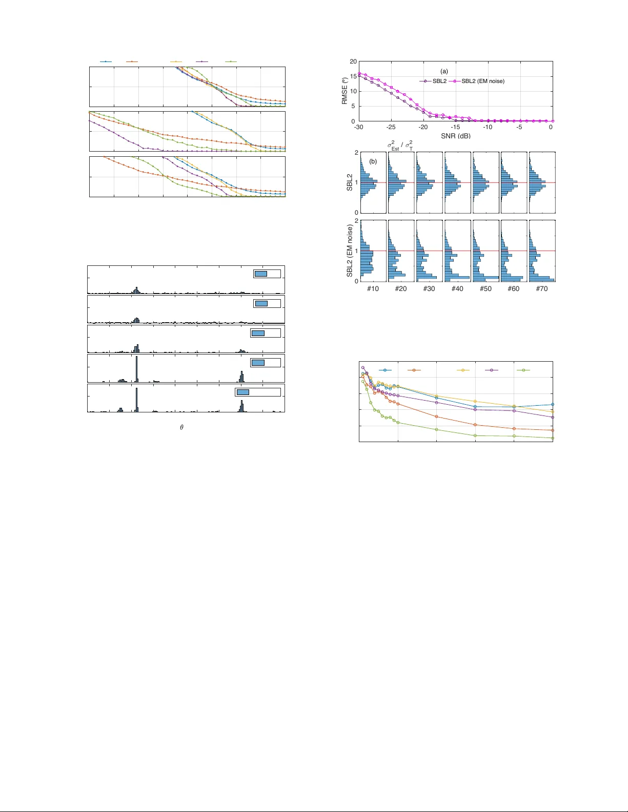
1 Sparse Bayesian Learning for DO A Estimation in Heteroscedastic Noise Peter Gerstoft Member , IEEE, Santosh Nannuru Member , IEEE, Christoph F . Mecklenbr ¨ auker Senior Member , IEEE, and Geert Leus F ellow , IEEE Abstract —November 13, 2017 The paper considers direction of arriv al (DO A) estimation from long-term observations in a noisy en vironment. In such an en vironment the noise source might evolv e, causing the stationary models to fail. Theref ore a heteroscedastic Gaussian noise model is introduced where the variance can vary across observations and sensors. The source amplitudes ar e assumed independent zero-mean complex Gaussian distributed with unkno wn v ariances (i.e. the source powers), inspiring stochastic maximum likelihood DO A estimation. The DO As of plane waves are estimated from multi-snapshot sensor array data using sparse Bayesian learning (SBL) where the noise is estimated acr oss both sensors and snapshots. This SBL approach is more flexible and performs better than high-resolution methods since they cannot estimate the heteroscedastic noise pr ocess. An alternative to SBL is simple data normalization, whereby only the phase across the array is utilized. Simulations demonstrate that taking the heteroscedastic noise into account improv es DOA estimation. Index T erms —Heteroscedastic noise, sparse reconstruction, array processing, DO A estimation, compressive beamforming, phase-only processing I . I N T R O D U C T I O N W ith long observ ation times weak signals can be extracted in a noisy environment. Most analytic treatments analyze these cases assuming Gaussian noise with constant v ariance. For long observation times the noise process though is likely to change with time causing the noise variance to ev olve. This is called a heteroscedastic Gaussian process, meaning that the noise variance is ev olving. While the noise variance is a nuisance parameter that we are not interested in, it still needs to be estimated or included in the processing in order to obtain an accurate estimate of the weaker signals. Accounting for the noise variation is certainly important for machine learning [1], [2] and related to robust statistics [3], [4]. Heteroscedastic noise models hav e been used in e.g. finance [5] and image processing [6]. In statistical signal pro- cessing, the noise has been assumed to v ary spatially [7], [8], [9], but spatiotemporally varying noise as considered here has not been studied. The proposed processing could be applied to spatial coherence loss [10], [11], [12] or to wavefront P . Gerstoft and S. Nannuru are with Univ ersity of California San Diego, La Jolla, CA 92093-0238, USA, http://noiselab .ucsd.edu C.F . Mecklenbr ¨ auker is with Institute of T elecommunications, V ienna Univ ersity of T echnology , 1040 V ienna, Austria, cfm@ieee.org G. Leus is with the Dept. of Electrical Eng., Math. and Comp. Science, Delft Univ . of T echnology , Delft, The Netherlands, g.j.t.leus@tudelft.nl Supported by the Office of Nav al Research, Grant Nos. N00014-1110439 and FTW Austria’ s “Compressed channel state information feedback for time- variant MIMO channels”. decorrelation, where turbulence causes the wa ve front to be incoherent for certain observations (thus more noisy). This has lead to so-called lucky imaging in astronomy [13] or lucky ranging in ocean acoustics [14], where only the measurements giving good results are used. As a result an inv olved hypothesis testing is needed to determine the measurements to be used. In contrast, we propose to use all measurements. In applications, a simple way to account for noise power variations is to normalize the data magnitude to only contain phase information as demonstrated for beamforming in seis- mology [15], [16], noise cross correlation in seismology [17], [18], [19], [20], [21] and acoustics [22], source decon volution in ocean acoustics [23], [24] and speaker localization [25], [26]. High-resolution beamformers such as MUSIC [27] rely- ing on a sample cov ariance matrix are not likely to perform well for heteroscedastic noise as the loud noise might dominate the sample co variance matrix. More adv anced methods than an eigen value decomposition are needed to separate the signal and noise subspaces. W e demonstrate that for well-separated sources normalizing the data to only contain phase information works well. When the sources are closely spaced, more advanced para- metric methods are needed for DO A estimation when the noise power is varying in space and time and the sources are weak. W e deriv e and demonstrate this for the application of multiple measurement vector (MMV , or multi-snapshot) compressive beamforming [28], [29], [30], [31]. W e solve the MMV prob- lem using the sparse Bayesian learning (SBL) framew ork [30], [32], [33] and use the maximum-a-posteriori (MAP) estimate for DOA reconstruction. W e assume the source signals to jointly follow a zero-mean multiv ariate complex normal distri- bution with unknown power le vels. The noise across sensors and snapshots also follows a zero-mean multi variate normal distribution with unknown variances. These assumptions lead to a Gaussian likelihood function. The corresponding posterior distribution is also Gaussian and already de veloped SBL approaches solve this well. W e base our development on our fast SBL method [32], [33] which we augment to estimate noise variances, potentially as many variances as observ ations. Standard techniques are based on minimization-majorization [34] and expectation maximization (EM) [30], [35], [36], [37], [38], [39], [40], though not all estimates work well. Instead, we estimate the unknown variances using stochastic maximum likelihood [41], [42], [43], modified to obtain noise estimates ev en for a single observation. 2 A. Heter oscedastic noise observation model For the l th observ ation snapshot, we assume the linear model y l = Ax l + n l , (1) where the dictionary A ∈ C N × M is constant and known, and the source vector x l ∈ C M contains the physical information of interest. Further, n l ∈ C N is additi ve zero-mean circularly symmetric complex Gaussian noise, which is generated from a heter oscedastic Gaussian process n l ∼ C N ( n l ; 0 , Σ n l ) . Due to the circular symmetry of the noise the phase is uniformly distributed. W e specialize to diagonal covariance matrices, parameter- ized as Σ n l = N X n =1 σ 2 nl J n = diag( σ 2 1 l , . . . , σ 2 N l ) , (2) where J n = diag( e n ) = e n e T n with e n the n th standard basis vector . Note that the cov ariance matrices Σ n l are varying over the snapshot index l = 1 , . . . , L and we introduce the matrix of all noise standard deviations as V N =    σ 11 . . . σ 1 L . . . . . . . . . σ N 1 . . . σ N L    ∈ R N × L 0+ , (3) where R 0+ denotes non-neg ati ve real numbers. W e consider three special cases for the a priori knowledge on the noise cov ariance model (2) which are expressed as constraints on V N . Case I W e assume wide-sense stationarity of the noise in space and time: σ 2 nl = σ 2 . The model is homoscedas- tic, V N ∈ V I = { V ∈ R N × L 0+ | V = σ 1 N 1 T L } . (4) Case II W e assume wide-sense stationarity of the noise in space only , i.e., the noise variance for all sensor elements is equal across the array , σ 2 nl = σ 2 0 l and it varies over snapshots. The noise v ariance is het- eroscedastic in time (across snapshots), V N ∈ V II = { V ∈ R N × L 0+ | V = ( σ 01 . . . σ 0 L ) 1 T L } . (5) Case III No additional constraints other than (3). The noise variance is heteroscedastic across both time and space (sensors and snapshots.). In this case V N ∈ V II I = R N × L 0+ . The relation between these noise cases is V I ⊂V II ⊂V II I = R N × L 0+ . From the sets V d ( d is I, II, or III) both V N in (3) and Σ n l in (2) can be constructed. B. Array model Let X = [ x 1 , . . . , x L ] ∈ C M × L be the complex source amplitudes, x ml = [ X ] m,l = [ x l ] m with m ∈ { 1 , · · · , M } and l ∈ { 1 , · · · , L } , at M DOAs (e.g., θ m = − 90 ◦ + m − 1 M 180 ◦ ) and L snapshots for a frequency ω . W e observe narrowband wa ves on N sensors for L snapshots Y = [ y 1 , . . . , y L ] ∈ C N × L . A linear regression model relates the array data Y to the source amplitudes X as Y = AX + N . (6) The dictionary A =[ a 1 ,..., a M ] ∈ C N × M contains the array steering vectors for all hypothetical DO As as columns, with the ( n, m ) th element giv en by e − j ωd n c sin θ m ( d n is the distance to the reference element and c the sound speed). W e assume M >N and thus (6) is underdetermined. In the presence of only few stationary sources, the source vector x l is K -sparse with K  M . W e define the l th activ e set M l = { m ∈ N | x ml 6 = 0 } , (7) and assume M l = M = { m 1 ,...,m K } is constant across all snapshots l . Also, we define A M ∈ C N × K which contains only the K “activ e” columns of A . In the following, k · k p denotes the vector p -norm and k · k F the matrix Frobenius norm. Similar to other DO A estimators, K can be estimated by model order selection criteria or by examining the angular spectrum. The parameter K is required only for the noise power in the SBL algorithm. An inaccurate estimate influences the algorithm’ s con ver gence. C. Prior on the sour ces W e assume that the complex source amplitudes x ml are in- dependent both across snapshots and across DO As and follow a zero-mean circularly symmetric complex Gaussian distribu- tion with DOA-dependent variance γ m , m = 1 , . . . , M , p ( x ml ; γ m ) = ( δ ( x ml ) , for γ m = 0 1 π γ m e −| x ml | 2 /γ m , for γ m > 0 , (8) p ( X ; γ γ γ γ γ ) = L Y l =1 M Y m =1 p ( x ml ; γ m ) = L Y l =1 C N ( x l ; 0 , Γ ) , (9) i.e., the source vector x l at each snapshot l ∈{ 1 , ··· ,L } is mul- tiv ariate Gaussian with potentially singular covariance matrix, Γ = diag ( γ γ γ γ γ ) = E [ x l x H l ; γ γ γ γ γ ] , (10) as rank( Γ )=card( M )= K ≤ M (typically K  M ). Note that the diagonal elements of Γ , denoted as γ γ γ γ γ , represent source powers and thus γ γ γ γ γ ≥ 0 . When the v ariance γ m =0 , then x ml =0 with probability 1. The sparsity of the model is thus controlled with the parameter γ γ γ γ γ , and the active set M is equiv alently M = { m ∈ N | γ m > 0 } . (11) The SBL algorithm ultimately estimates γ γ γ γ γ rather than the complex source amplitudes X . This amounts to a significant reduction of the de grees of freedom resulting in a low v ariance of the DOA estimates. D. Stochastic likelihood W e here derive the well-known stochastic maximum like- lihood function [44], [45], [46]. Giv en the linear model (6) with Gaussian source (9) and noise (2) the array data Y is 3 Gaussian with for each snapshot l the covariance Σ y l giv en by Σ y l = E [ y l y H l ] = Σ n l + AΓA H (12) The probability density function of Y is thus gi ven by p ( Y ) = L Y l =1 C N ( y l ; 0 , Σ y l ) = L Y l =1 e − y H l Σ − 1 y l y l π N det Σ y l . (13) The L -snapshot log-likelihood for estimating γ γ γ γ γ and V N is log p ( Y ; γ γ γ γ γ , V N ) ∝ − L X l =1  y H l Σ − 1 y l y l + log det Σ y l  . (14) This likelihood function is identical to the T ype II likelihood function (evidence) in standard SBL [36], [35], [32] which is obtained by treating γ γ γ γ γ as a hyperparameter . The T ype II likelihood is obtained by integrating the likelihood function ov er the complex source amplitudes, cf. (29) in [32]. The stochastic maximum likelihood approach is used here as it is more direct. The parameter estimates ˆ γ γ γ γ γ and b V N are obtained by maxi- mizing the likelihood, leading to (ˆ γ γ γ γ γ , b V N ) = arg max γ ≥ 0 , V N ∈V d log p ( Y ; γ γ γ γ γ , V N ) , (15) where V d is the feasible set of noise variances V N in (3) corresponding to the noise cases ( d = I, II, or III, see Sec. I-A).The likelihood function (14) is similar to the ones deriv ed for SBL and LIKES [34]. If γ γ γ γ γ and Σ n l are kno wn, then the MAP estimate is the posterior mean ˆ x MAP l and cov ariance Σ x l [47], [32], ˆ x MAP l = ΓA H Σ − 1 y l y l , (16) Σ x l =  A H Σ − 1 n l A + Γ − 1  − 1 . (17) The diagonal elements of Γ , i.e., γ γ γ γ γ , control the row-sparsity of ˆ x MAP l as for γ m = 0 the corresponding m th ro w of ˆ x MAP l becomes 0 T . E. LASSSO versus SBL Both LASSO and SBL use the linear model (6) with complex zero-mean Gaussian random noise but they differ in the modeling of the source matrix X . The LASSO approach assumes a priori X random with uniformly i.i.d. distributed phase and Laplace-like prior am- plitudes, p ( X ) = p ( x ` 2 ) ∝ exp( −k x ` 2 k 1 /ν ) , (18) [ x ` 2 ] n = L X l =1 | [ x l ] n | 2 ! 1 / 2 . (19) Thus only the summed amplitudes (19) are Laplacian. The elements in X are unkno wn and must be estimated. The LASSO approach uses the conditional likelihood (T ype I) for p ( Y | X ) and applies Bayes rule with the prior p ( X ) gi ving the MAP estimate b X = arg max p ( Y | X ) p ( X ) = arg min X ∈ C N × L k Y − AX k 2 F + µ k x ` 2 k 1 . (20) The LASSO approach (20) estimates the realization of x l for each snapshot l . The number of parameters to be estimated for the LASSO approach grows linearly with the number of snapshots. The SBL approach on the other hand, assumes that e v- ery column of X is random with the same complex zero- mean Gaussian a priori distribution C N ( x l ; 0 , Γ ) . The SBL approach uses the likelihood p ( Y | γ γ γ γ γ , Σ N ) in (15) and estimates γ γ γ γ γ but not the realization of X . Therefore, the number of pa- rameters to be estimated for the SBL approach is independent of the number of snapshots. Thus the quality of the estimate improv es faster than with LASSO. For the heteroscedastic noise model, a dif ferent covariance matrix could be included in the data fit of (20). Ho wever , since the number of parameters to be estimated gro ws with the number of snapshots, this seems less attracti ve than using SBL. F . Pr e-whitening The purpose of this section is to moti vate the empirical evidence [15]–[26] that phase-only processing might provide improv ed estimates over using also amplitudes. This is most likely to happen when sources are not closely spaced and at low SNR as demonstrated in the examples, Sec. V. Let us introduce the factorization Σ − 1 n l = W H l W l , where W l is a square and non-singular matrix. For our particular setup, we have W l = diag( σ − 1 1 l , . . . , σ − 1 N l ) . The matrix W l is useful for pre-whitening the sensor data. The corresponding whitened sensor data and dictionary matrix are e y l = W l y l , (21a) e A l = W l A . (21b) For kno wn diagonal noise covariance Σ n l the above means we hav e to normalize each ro w in (1) with σ nl as then the noise satisfies e n l ∼ C N ( e n l ; 0 , I ) , and thus all entries are identically distributed. If the noise cov ariance matrices are not kno wn, the y can be estimated as we will show later on. More specifically , at low SNR, the Noise Cases I, II, and III, lead to the noise variance estimates (43), (44). The corresponding pre-whitening matrices can then be computed as W l ≈      √ N L k Y k F I for Case I √ N k y l k 2 I for Case II diag ( | y 1 ,l | , . . . , | y N ,l | ) − 1 for Case III , (22) leading to e y l ≈      √ N L k Y k F y l for Case I √ N k y l k 2 y l for Case II [ y 1 ,l / | y 1 ,l | , . . . , y N ,l / | y N ,l | ] T for Case III . (23) Empirically , it has been found that applying pre-whitening to the data y l only (the dictionary A is non-whitened) ef fectiv e in finding the strongest DO A. 4 For Noise Case I, pre-whitening does not play a role and the con ventional beamformer is formulated using the po wer spectrum at DOA θ m P CBF ( θ m ) = 1 L a H m YY H a m = a H m S y a m , (24) where the sample cov ariance matrix is S y = 1 L YY H . (25) For Noise Cases II and III on the other hand, we will work with the pre-whitened data. In those cases, , the con ventional beamformer leads to the po werspectra P CBF2 and P CBF-Phase , respectiv ely , which can be formulated as P CBF* ( θ m ) = 1 L a H m ˜ Y ˜ Y H a m = a H m S ˜ y a m , (26) where the whitened sample cov ariance matrix is S ˜ y = 1 L e Y e Y H = 1 L L X l =1 y l W 2 l y H l . (27) The weighting W l is given by (22). For Case III, only phase is used as can be observed from (23), which results in phase- only processing. As demonstrated in Section V -B this simple pre-whitening can improve the DOA performance at low SNR. I I . S O U R C E P OW E R E S T I M A T I O N Let us no w focus on the SBL algorithm solving (15). The algorithm iterates between the source power estimates ˆ γ γ γ γ γ deri ved in this section and the noise variance estimates b V N computed in Sec. III. After detailing these estimation procedures, the full algorithm is summarized in Sec. IV. W e impose the diagonal structure Γ =diag ( γ γ γ γ γ ) , in agreement with (9), and form deriv ati ves of (14) with respect to the diagonal elements γ m , cf. [44]. Using ∂ Σ − 1 y l ∂ γ m = − Σ − 1 y l ∂ Σ y l ∂ γ m Σ − 1 y l = − Σ − 1 y l a m a H m Σ − 1 y l , (28) ∂ log det( Σ y l ) ∂ γ m = tr  Σ − 1 y l ∂ Σ y l ∂ γ m  = a H m Σ − 1 y l a m , (29) the deri vati ve of (14) is formulated as ∂ log p ( Y ; γ γ γ γ γ , V N ) ∂ γ m = L X l =1  a H m Σ − 1 y l y l y H l Σ − 1 y l a m − a H m Σ − 1 y l a m  = L X l =1 a H m  Σ − 1 y l y l y H l Σ − 1 y l − Σ − 1 y l  a m (30) = L X l =1 | y H l Σ − 1 y l a m | 2 − L X l =1 a H m Σ − 1 y l a m . (31) For the solution to (15), we impose the necessary condition ∂ log p ( Y ; γ , V N ) ∂ γ m = 0 . T o obtain an iterative equation in γ m , we multiply the first term in the above equation with the factor ( γ old m γ new m ) 1 /b , whereby ( γ old m γ new m ) 1 /b L X l =1 | y H l Σ − 1 y l a m | 2 − L X l =1 a H m Σ − 1 y l a m = 0 . (32) Assuming γ old m and Σ y l giv en (from pre vious iterations or initialization) and forcing (32) to zero, we obtain the following fixed point iteration [48] for the γ m : γ new m = γ old m P L l =1 | y H l Σ − 1 y l a m | 2 P L l =1 a H m Σ − 1 y l a m ! b . (33) W e use b = 0 . 5 , but have not carefully tested for optimal values and this value depends on many factors such as which noise estimate is used and closeness of the DO As. A value of b = 1 giv es the update equation used in [47], [30], [33] and b = 0 . 5 giv es the update equation used in [32]. I I I . N O I S E V A R I A N C E E S T I M A T I O N While there has been more focus on estimating the DOAs or γ γ γ γ γ , noise is an important part of the physical system and a correct estimate is needed for good con ver gence properties. In SBL, the noise variance controls the sharpness of the peaks in the γ γ γ γ γ spectrum, with higher noise lev els giving broader peaks. Thus, as we optimize the DO As we expect the noise lev els to decrease and the γ γ γ γ γ spectrum to become sharper . In this section we estimate the noise variance for the three noise cases in Sec. I-A. In Secs. III-A – III-C, we will assume the support of γ γ γ γ γ is known. A. Noise estimate, Case I Under Noise Case I, where Σ n l = σ 2 I N with I N the identity matrix of size N , stochastic maximum likelihood [38], [41], [43] can provide an asymptotically efficient estimate of σ 2 if the set of activ e DO As M is known. Let Γ M =diag( γ γ γ γ γ new M ) be the co variance matrix of the K ac- tiv e sources obtained abov e with corresponding active steering matrix A M which maximizes (14). The corresponding data cov ariance matrix is Σ y l = σ 2 I N + A M Γ M A H M . (34) Note that for Noise Case I, the data cov ariance matrices (12) and (34) are identical. Follo wing [42], we continue from (30), ∂ log p ( Y ; γ γ γ γ γ , V N ) L ∂ γ m = a H m  Σ − 1 y l S y Σ − 1 y l − Σ − 1 y l  a m (35) = a H m Σ − 1 y l ( S y − Σ y l ) Σ − 1 y l a m = 0 , (36) for all acti ve sources ( m ∈ M ). Since range( Σ − 1 y l A M ) = range( A M ) , Eq.(36) simplifies to a H m ( S y − Σ y l ) a m = 0 , ∀ m ∈ M . (37a) T o obtain Jaffer’ s condition below , we impose the following additional constrains a H m ( S y − Σ y l ) a p = 0 , ∀ m, p ∈ M , m 6 = p. (37b) T ogether , the conditions (37a), (37b) gi ve Jaffer’ s condition ([42]:Eq.(6)), i.e., A H M ( S y − Σ y l ) A M = 0 , (38) which we enforce at the optimal solution ( Γ M , σ 2 ) . Jaffer’ s condition follo ws from allo wing arbitrary correlations among 5 the source signals, i.e. when the Γ matrix is not restricted to be diagonal. Substituting (34) into (38) gives A H M  S y − σ 2 I N  A M = A H M A M Γ M A H M A M . (39) Let us then define the projection matrix onto the subspace spanned by the activ e steering vectors P = A M A + M = A M ( A H M A M ) − 1 A H M = P H = P 2 . (40) Left-multiplying (39) with A + H M = A M ( A H M A M ) − 1 and right-multiplying it with A + M =( A H M A M ) − 1 A H M , we obtain PS y P H − σ 2 PP H = P A M Γ M A H M P H = A M Γ M A H M = Σ y l − σ 2 I N . (41) Evaluating the trace, using tr  PP H  = K and tr  PS y P H  = tr( PS y ) , gi ves σ 2 = tr[ Σ y l − PS y ] N − K = tr[( S y − PS y ] +  N − K (42) ≈ tr[( I N − P ) S y ] N − K = ˆ σ 2 , (43) where we have defined  =tr[ Σ y l − S y ] . The abo ve approximation motiv ates the noise po wer esti- mate for Noise Case I (43), which is err or-fr ee if tr[ Σ y ]= tr[ S y ] , unbiased because E [  ] = 0 , consistent since also its variance tends to zero for L →∞ [49], and asymptotically efficient as it approaches the CRLB for L →∞ [50]. Note that, the Noise Case I estimate (43) is v alid for any number of snapshots, e ven for just one snapshot. B. Noise estimate, Case II For Noise Case II, where Σ l = σ 2 l I N , we apply (43) for each snapshot l individually , leading to ˆ σ 2 l = tr[( I N − P ) y l y H l ] N − K = k ( I N − P ) y l k 2 2 N − K . (44) Sev eral alternativ e estimators for the noise variance are pro- posed based on EM [36], [30], [37], [47], [51]. For a compar- ativ e illustration in Sec. V -D1 we will use the iterative noise estimate from [36], giv en by ( σ 2 l ) new = || y l − A b x MAP l || 2 F + ( σ 2 l ) old ( M − P M i =1 ( Σ x l ) ii γ i ) N , (45) where the posterior mean b x MAP l and cov ariance Σ x l are giv en in (16) and (17). Empirically , EM noise estimates such as (45) significantly underestimate the true noise variance in our applications. C. Noise estimate, Case III Let us start from the definition of the noise cov ariance Σ n l = E  ( y l − Ax l )( y l − Ax l ) H  = E  ( y l − A M x M ,l )( y l − A M x M ,l ) H  . (46) This motiv ates plugging-in the single-observation signal esti- mate b x M ,l = A + M y l ∈ C K for the active (non-zero) entries in x l . This estimate is based on the single observ ation y l and the projection matrix (40), giving the rank-1 estimate b Σ n l = ( I − P ) y l y H l ( I − P ) . (47) Since the signal estimate b x M ,l maximizes the estimated signal power , this noise cov ariance estimate is biased and the noise lev el is likely underestimated. Since we assume the noise independent across sensors, all off-diagonal elements of Σ n l are kno wn to be zero. With this constraint in mind, we modify (47) as b Σ n l = diag[ σ 2 1 l , . . . , σ 2 nl , . . . , σ 2 N l ] = diag  diag  ( I − P ) y l y H l ( I − P )  . (48) The estimate (48) is demanding as for all the N × L complex- valued observ ations in Y , we obtain N × L estimates of the noise variance. Note that the estimate b Σ n l in (47) is not in vertible whereas the diagonal constraint in (48) leads to a non-singular estimate of Σ n l with high probability (it is singular only if an element of y l is 0 ). As a result, the expression for Σ y l that is used for estimating γ γ γ γ γ in (33) is likely inv ertible. On the other hand, an overestimate of the noise is easily obtained by assuming x l = 0 which is equiv alent to setting P = 0 in (48), resulting in b Σ n l = diag  diag  y l y H l  (49) or b σ nl = | y nl | . (50) This can be shown be the maximum likelihood estimate for no sources ( M = 0 ) or very lo w po wer sources. I V . S B L A L G O R I T H M The complete SBL algorithm is summarized in T able I. The same algorithm is valid for Noise Cases I, II, and III (at high SNR). Gi ven the observed Y , we iterati vely update Σ y l (12) by using the current γ γ γ γ γ and Σ n l . The Σ − 1 y l is computed directly as the numerical in verse of Σ y l . For updating γ m , m = 1 , . . . , M we use (33). For the initialization of γ γ γ γ γ we use the con ventional beamformer (CBF) po wer γ γ γ γ γ = diag[ A H S y A ] . (51) Based on the corresponding noise case, (43), (44), (45), or (48) is used to estimate Σ n l . The noise is initialized using (43), (44), (45), or (48) with P = 0 , K = 0 , which provides an ov er estimate of the noise variance. The con vergence rate  measures the relativ e change in estimated total source power ,  = k γ γ γ γ γ new − γ γ γ γ γ old k 1  k γ γ γ γ γ old k 1 . (52) The algorithm stops when  ≤  min and the output is the activ e set M (see (11)) from which all source parameters are computed. 6 0 Initialize: γ γ γ γ γ new = diag[ A H S y A ] , Σ new n l = Eq. (43), (44), (45), or (48) with P = 0 , K = 0  min = 0 . 001 ,  = 2  min , j = 0 , j max = 100 1 while (  >  min ) and ( j < j max ) 2 γ γ γ γ γ old = γ γ γ γ γ new , Γ = diag( γ γ γ γ γ old ) , Σ old n l = Σ new n l 3 Σ y l = Σ old n l + AΓA H (12) 4 γ new m use (33) 5 M = { m ∈ N | K largest peaks in γ γ γ γ γ } = { m 1 . . . m K } (11) 6 A M = ( a m 1 , . . . , a m K ) , P = A M A + M 7 Σ new n l = choose from (43), (44), (45), or (48) 8  = k γ γ γ γ γ new − γ γ γ γ γ old k 1 / k γ γ γ γ γ old k 1 , j = j + 1 (52) 9 Output: M , γ γ γ γ γ new , Σ new n l T ABLE I S B L A L G O RI T H M . a) 5 10 15 20 b) 5 10 15 20 25 30 35 40 45 50 Snapshot # 5 10 15 20 Sensor # 0 0.5 1 1.5 2 2.5 3 3.5 4 0 0.5 1 1.5 2 2.5 3 3.5 4 Standard deviation 0 20 40 60 80 Bin count c) Fig. 1. Noise standard deviation matrix V N in (3) for Noise Cases a) II and b) III. c) Histogram of noise for Noise Case III with log 10 σ nl ∼ U ( − 1 , 1) . In both cases the standard deviation has mean 1. V . E X A M P L E S When the noise process is stationary and only one source is acti ve, the peak of the CBF spectrum provides the optimal estimate of the source location. With heteroscedastic noise this may not hold true. W e propose to use a robust CBF (Sec.V -B) or find the DO A with SBL, which takes the heteroscedastic noise into account (Sec. V -C). W ith multiple sources and heteroscedastic noise we use SBL (Sec. V -D). A. Simulation setup In the analysis of seismic data the noise for each snapshot was observed to be log-normal distributed [52]. Noise has also been modeled with extreme distributions [53]. In the simulations here, the noise follows a normal-uniform hierar- chical model. The noise is complex zero-mean Gaussian with the noise standard deviation uniformly distributed ov er two decades, i.e., log 10 σ nl ∼U ( − 1 , 1) , where U is the uniform dis- tribution. Three noise cases are simulated: (a) Case I: constant noise standard deviation over snapshots and sensors, (b) Case II: standard deviation changes across snapshots with log 10 σ l ∼ U ( − 1 , 1) , and (c) Case III: standard deviation changes across both snapshots and sensors with log 10 σ nl ∼U ( − 1 , 1) . A realization of the noise standard deviation is sho wn for Noise Cases II (Fig. 1a) and III (Fig. 1b) for N =20 sensors and L =50 snapshots. The corresponding histogram is presented in Fig. 1c. B. Single DO A with CBF and MUSIC The single source is located at − 3 ◦ . The complex source amplitude is stochastic and there is additi ve heteroscedastic Gaussian noise with SNR variation from − 40 to 0 dB. The sensor array has N =20 elements with half wav elength spac- ing. W e process L =50 snapshots. The angle space [ − 90 , 90] ◦ is di vided into a 0 . 5 ◦ grid ( M =360 ). The single-snapshot array signal-to-noise ratio (SNR) is SNR=10log 10 [ E  k Ax l k 2 2  / E  k n l k 2 2  ] . (53) W e first compute the beam spectra using CBF (24), CBF2 and CBF-Phase both (26) b ut with different weighting (23). When the noise is homoscedastic (constant standard devia- tion), the beam spectra for the three processors behav e simi- larly (first ro w in Fig. 2). For heteroscedastic noise CBF2 and CBF-Phase give much better discrimination between signal to noise, see Fig. 2 middle (Noise Case II) and bottom ro w (Noise Case III). The root mean squared error (RMSE) of the DO A estimates ov er N sim =100 runs with random noise realizations is used for ev aluating the algorithm RMSE = v u u t N sim X n =1 K X i =1 ( ˆ θ n i − θ 0 i ) 2 N sim K , (54) where θ 0 i is the true DO A and ˆ θ n i is the estimated DO A for the i th source when K sources are present. -12 -8 -4 0 SNR = -10 dB Noise Case I SNR = -25 dB Noise Case I CBF CBF2 CBF-Phase -12 -8 -4 0 Noise Case II Noise Case II -20 0 20 40 60 80 Angle ( ° ) -12 -8 -4 0 Power (dB) Noise Case III -20 0 20 40 60 80 Angle ( ° ) Noise Case III Fig. 2. Beam spectra for source at − 3 ◦ for SNR − 10 dB (left) and − 25 dB (right) for CBF (black), CBF2 (red), CBF-Phase (blue). The noise standard deviation is a) constant or heteroscedastic with either b) log 10 σ l ∼ U ( − 1 , 1) or c) log 10 σ nl ∼ U ( − 1 , 1) . 20 elements and 50 snapshots based on one simulation are used. 7 0 10 20 (a) Noise Case I 0 10 20 (b) Noise Case II -40 -35 -30 -25 -20 -15 -10 -5 0 SNR (dB) 0 10 20 RMSE ( ° ) (c) Noise Case III CBF CBF2 CBF-Phase MUSIC Fig. 3. Single source at θ = − 3 ◦ : Array RMSE using beamforming with pre-whitening for Noise Cases (a) I, (b) II, and (c) III. Each noise case is solved with CBF , CBF2, CBF-Phase, and MUSIC. 0 10 20 (a) Noise Case I CBF CBF-Phase SBL SBL2 SBL3 BP 0 10 20 RMSE ( ° ) (b) Noise Case II -40 -35 -30 -25 -20 -15 -10 -5 0 SNR (dB) 0 10 20 (c) Noise Case III Fig. 4. Single source at − 3 ◦ : RMSE vs. SNR for DOA estimation using various algorithms for Noise Cases (a) I, (b) II, and (c) III. The SNR curves (Fig. 3) demonstrate increased robustness of CBF2 and CBF-Phase, failing 20 dB later . Due to the heteroscedastic noise, MUSIC performs worse than CBF for a single source. CBF-Phase di ver ges at an SNR 15–20 dB later than CBF for Noise Cases II and III. C. Single DO A estimation with SBL W e use the follo wing SBL methods, with γ γ γ γ γ update (33) and SBL: Solves Case I using standard SBL, with σ from (43). SBL2: Solves Case II, with σ l for each snapshot from (44). SBL3: Solves Case III, with σ nl from (48). In addition to these methods we also use basis pursuit (BP) as implemented in [31]. For Noise Case I, all the methods fail near the same SNR of − 12 . 5 dB, Fig. 4a. When the noise is heteroscedastic across snapshots, CBF , BP , and SBL fail early . Since both SBL2 and SBL3 correctly model the noise, the y perform the best for Noise Case II, Fig. 4b. CBF-Phase also performs well. For heteroscedastic Noise Case III, SBL3 fails the last and as before CBF-Phase also performs well. SBL3 fails 15 dB later than any other method. This demonstrates the usefulness of accurate noise models in DO A processing. 0 50 CBF 0 50 SBL 0 50 Bin count SBL2 0 50 SBL3 Noise Case III, SNR =-25 dB -30 -20 -10 0 10 20 ( ° ) 0 50 CBF-Phase Fig. 5. Single source at − 3 ◦ : Histogram of the peak location for Noise Case III at SNR − 25 dB. (a) True Noise 5 10 15 20 0 0.5 1 1.5 2 2.5 (b) Avg. Noise 5 10 15 20 Sensor # (c) Example Noise 10 20 30 40 50 Snapshot # 5 10 15 20 0 5 10 15 20 Sensor # 0 0.5 1 1.5 std. dev. (d) True Estimated Fig. 6. Single source at − 3 ◦ , SNR= 0 dB: SBL3 noise standard deviation matrix V N in (3): (a) true standard deviations, (b) average estimated (500 simulations) standard deviations, (c) a typical estimate of standard deviations, and (d) average standard de viations across simulations and snapshots. The histograms (Fig. 5) of the DOA (location of peak in po wer spectrum) at SNR − 25 dB for Noise Case III demonstrate that when the heteroscedastic noise is accounted for , the histograms concentrate near the true DO A ( θ = − 3 ◦ ). An example statistic of the heteroscedastic noise standard deviation is sho wn in Fig. 6. The standard deviation for each sensor is either 0 or √ 2 . SBL3 estimates the standard de viation from (48). A verage noise in Fig. 6b resembles well the true noise (Fig. 6a) whereas the sample estimate (Fig. 6c) has high variance. Fig. 6d plots the mean across simulations and snapshots of the estimated standard deviation. On average, the noise estimate is close to the true noise. 8 0 10 20 (a) Noise Case I CBF CBF-Phase SBL SBL2 SBL3 0 10 20 RMSE ( ° ) (b) Noise Case II -30 -25 -20 -15 -10 -5 0 5 10 SNR (dB) 0 10 20 (c) Noise Case III Fig. 7. RMSE vs. SNR with the three sources at {− 3 ◦ , 2 ◦ , 50 ◦ } and power { 10 , 22 , 20 } dB. 0 50 CBF 0 50 SBL 0 50 Bin count SBL2 0 50 SBL3 Noise Case III, SNR =-15 dB -20 -10 0 10 20 30 40 50 60 70 ( ° ) 0 50 CBF-Phase Fig. 8. Three sources at {− 3 ◦ , 2 ◦ , 50 ◦ } : Histogram of the top three peak locations for Noise Case III at SNR − 15 dB. D. Three DO A estimation with SBL Now consider three sources located at [ − 3 , 2 , 50] ◦ with power [10 , 22 , 20] dB, see Fig. 7. Relativ e to the single source case, the CBF-Phase performs significantly worse than SBL3, as the sources at − 3 ◦ and 2 ◦ are both in the CBF main lobe. The localization ability of the algorithms can also be gauged from the histogram of the top three peaks, see Fig. 8. Since SBL3 accounts for the heteroscedastic Noise Case III, its histogram is concentrated near the true DOAs. 1) Noise estimate con verg ence: The performance of the SBL methods is strongly related to the accuracy of the noise estimates. For the l th snapshot, the true noise power σ 2 l,T (Noise Case II) is σ 2 l,T = E [ k n l k 2 2 ] / N = 10 − SNR / 10 E [ k Ax l k 2 2 ] / N . (55) The estimated ( σ 2 l ) new (44) de v i ates from σ 2 l,T (55) randomly . W e also consider the noise estimate (45) based on the EM method. Fig. 9 compares the two noise estimates for noise generated with log σ l ∼ U ( − 1 , 1) . The ev olution of the his- tograms of the relati ve noise v ariance σ 2 Est /σ 2 T with iterations is in Fig. 9b. The mean of the ratio of σ 2 Est /σ 2 T is close to 1 for SBL2 but is much lo wer for the EM noise estimate (45), this likely causes the SBL2 (EM noise, (45)) to fails 5 dB earlier . -30 -25 -20 -15 -10 -5 0 SNR (dB) 0 5 10 15 20 RMSE ( ° ) (a) SBL2 SBL2 (EM noise) 0 1 2 SBL2 < 2 Est / < 2 T (b) 0 1 2 SBL2 (EM noise) #10 #20 #30 #40 #50 #60 #70 Fig. 9. Three sources at {− 3 ◦ , 2 ◦ , 50 ◦ } (Noise Case II): (a) RMSE vs. SNR for SBL2 with two noise estimates. (b) Evolution of histogram of noise variance σ 2 Est /σ 2 T for SBL2 (44) and SBL2 with EM noise estimate (45) with iterations at SNR − 10 dB. 0 10 20 30 40 50 # Snapshots 0 5 10 15 20 25 RMSE ( ° ) Noise Case III, SNR =-5 dB CBF CBF-Phase SBL SBL2 SBL3 Fig. 10. Three sources at {− 3 ◦ , 2 ◦ , 50 ◦ } (Noise Case III): RMSE vs. Number of snapshots with SNR − 5 dB. 2) Number of snapshots: The RMSE versus number of snapshots for Noise Case III (Fig. 10) shows that SBL3 is most accurate with CBF-Phase following. 3) Noise distribution: For Noise Case III, we are just using one observation to estimate the standard deviation for SBL3 (48). Thus the estimates are not good, see Fig. 11. The true noise standard deviation is generated from log 10 σ T ,nl ∼ U ( − 1 , 1) , see Fig. 11a. The distribution of the deviation from the true standard deviation σ Est − σ T (Fig. 11c) is well-centered (mean 0.007). V I . C O N C L U S I O N Likelihood based methods for single and multiple DO A estimation from long-term observ ations corrupted by non- stationary additi ve noise are discussed. In such a setting, the DOA estimators for a stationary noise model perform poorly . Therefore a heteroscedastic Gaussian noise model is introduced where the noise v ariance v aries across sensors and snapshots. W e develop Sparse Bayesian Learning (SBL) 9 a)True, SNR=0 0 1 2 3 4 5 6 7 8 9 10 T 0 100 200 300 b) Estimated 0 1 2 3 4 5 6 7 8 9 10 Est 0 50 100 150 c) Deviation -5 -4 -3 -2 -1 0 1 2 3 4 5 Est - T 0 50 100 150 Fig. 11. Three sources at {− 3 ◦ , 2 ◦ , 50 ◦ } (Noise Case III): Histogram of noise for a realization for SBL3 with 50 snapshots and 20 sensors (1000 observations) with SNR 0 dB. a) True σ T , b) estimated σ Est , and c) deviation σ Est − σ T . approaches to estimate source powers, source DOAs, and the noise v ariance parameters. Simulations show that normalizing the array data magnitude (such that only the phase information is retained) is simple and useful for estimating a single source in heteroscedastic Gaussian noise. For the estimation of (multiple) closely spaced sources, a problem specific SBL approach gi ves a much lower RMSE in the DO A estimates. R E F E R E N C E S [1] K. P . Murphy . Machine learning: a probabilistic perspective . MIT press, 2012. [2] C. M. Bishop. P attern reco gnition and machine learning . Springer, 2006. [3] P . J. Huber. Robust statistics . Springer , 2011. [4] R. Maronna, D. Martin, and V . Y ohai. Robust statistics . John W iley , Chichester ., 2006. [5] R. F . Engle. Autoregressi ve conditional heteroscedasticity with estimates of the variance of united kingdom inflation. Econometrica , pages 987– 1007, 1982. [6] T .H. Thai, R. Cogranne, and F Retraint. Camera model identification based on the heteroscedastic noise model. IEEE T rans. Image Proc. , 23(1):250–263, 2014. [7] M. V iberg, P . Stoica, and B. Ottersten. Maximum likelihood array pro- cessing in spatially correlated noise fields using parameterized signals. IEEE Tr ans Signal Pr oc. , 45(4):996–1004, 1997. [8] C. E. Chen, F . Lorenzelli, R.E Hudson, and K. Y ao. Stochastic maximum-likelihood doa estimation in the presence of unknown nonuni- form noise. IEEE T rans. Signal Pr oc. , 56(7):3038–3044, 2008. [9] T Li and A. Nehorai. Maximum likelihood direction finding in spatially colored noise fields using sparse sensor arrays. IEEE T rans Signal Proc. , 59(3):1048–1062, 2011. [10] H. Cox. Line array performance when the signal coherence is spatially dependent. J Acoust. Soc. Am. , 54(6):1743–1746, 1973. [11] A. Paulraj and T . Kailath. Direction of arrival estimation by eigenstruc- ture methods with imperfect spatial coherence of wave fronts. J Acoust. Soc. Am. , 83(3):1034–1040, 1988. [12] R. Lefort, R. Emmeti ` ere, S. Bourmani, G. Real, and A. Dr ´ emeau. Sub- antenna processing for coherence loss in underwater direction of arriv al estimation. J Acoust. Soc. Am. , 142(4):2143–2154, 2017. [13] N.M Law , C. D. Mackay , and J.E Baldwin. Lucky imaging: high angular resolution imaging in the visible from the ground. Astr onomy & Astrophysics , 446(2):739–745, 2006. [14] H. Ge and I. P . Kirsteins. Lucky ranging with to wed arrays in underwater en vironments subject to non-stationary spatial coherence loss. In IEEE Intl. Conf. Acoust., Speech and Signal Pr oc. (ICASSP) , pages 3156– 3160, 2016. [15] P . Gerstoft, M. C. Fehler, and K. G. Sabra. When katrina hit california. Geophys. Res. Lett. , 33(17), 2006. [16] P . Gerstoft and P . D. Bromirski. “Weather bomb” induced seismic signals. Science , 353(6302):869–870, 2016. [17] P . Roux, K. G. Sabra, P . Gerstoft, W . A. Kuperman, and M. C. Fehler . P-wav es from cross-correlation of seismic noise. Geophys. Res. Lett. , 32(19), 2005. [18] N. Harmon, P . Gerstoft, C. A. Rychert, G. A. Abers, M. Salas de La Cruz, and K. M. Fischer . Phase velocities from seismic noise using beamforming and cross correlation in Costa Rica and Nicaragua. Geophy . Res. Lett. , 35(19), 2008. [19] M. Land ` es, F . Hubans, N. M Shapiro, A. Paul, and M. Campillo. Origin of deep ocean microseisms by using teleseismic body waves. J. Geophys Res: Solid Earth , 115(B5), 2010. [20] Z. Zhan, S. Ni, D. V Helmberger , and R. W . Clayton. Retriev al of moho- reflected shear wav e arrivals from ambient seismic noise. Geophys. J. Int. , 182(1):408–420, 2010. [21] C. W eemstra, W . W estra, R. Snieder, and L. Boschi. On estimating attenuation from the amplitude of the spectrally whitened ambient seismic field. Geophys. J . Int. , 197(3):1770–1788, Apr 2014. [22] P . Gerstoft, W . S. Hodgkiss, M. Siderius, C.-F . Huang, and C.H. Harri- son. Passiv e fathometer processing. J. Acoust. Soc. Am. , 123(3):1297– 1305, 2008. [23] K.G. Sabra and D.R. Dowling. Blind deconv olution in ocean wa veguides using artificial time reversal. J. Acoust. Soc. Am. , 116(1):262–271, 2004. [24] K.G. Sabra, H-C. Song, and D.R. Dowling. Ray-based blind deconv olu- tion in ocean sound channels. J . Acoust. Soc. Am. , 127(2):EL42–EL47, 2010. [25] O. Schwartz and S. Gannot. Speaker tracking using recursi ve em algorithms. IEEE T rans. Audio, Speech, Language Pr oc. , 22(2):392– 402, 2014. [26] Y Dorfan and S Gannot. T ree-based recursive expectation-maximization algorithm for localization of acoustic sources. IEEE T rans. Audio, Speech and Lang. Pr oc. , 23(10):1692–1703, 2015. [27] H.L. V an T rees. Optimum Array Processing , chapter 1–10. W iley- Interscience, New Y ork, 2002. [28] D. Malioutov , M. C ¸ etin, and A. S. Willsky . A sparse signal reconstruc- tion perspectiv e for source localization with sensor arrays. IEEE T rans. Signal Process. , 53 (8):3010–3022, 2005. [29] A. Xenaki, P . Gerstoft, and K. Mosegaard. Compressiv e beamforming. J. Acoust. Soc. Am. , 136 (1):260–271, 2014. [30] D. P . Wipf and B.D. Rao. An empirical Bayesian strategy for solving the simultaneous sparse approximation problem. IEEE T rans. Signal Pr oc. , 55 (7):3704–3716, 2007. [31] P . Gerstoft, A. Xenaki, and C.F . Mecklenbr ¨ auker . Multiple and single snapshot compressive beamforming. J. Acoust. Soc. Am. , 138(4):2003– 2014, 2015. [32] P . Gerstoft, C. F . Mecklenbr ¨ auker , A. Xenaki, and S. Nannuru. Multi- snapshot sparse Bayesian learning for DOA. IEEE Signal Pr oc. Lett. , 23(10):1469–1473, 2016. [33] S. Nannuru, K.L Gemba, P . Gerstoft, W .S. Hodgkiss, and C.F . Meck- lenbr ¨ auker . Sparse Bayesian learning with uncertainty models and multiple dictionaries. , 2017. [34] P . Stoica and P . Babu. SPICE and LIKES: T wo hyperparameter-free methods for sparse-parameter estimation. Signal Pr oc. , 92(7):1580– 1590, 2012. [35] D. P . W ipf and S. Nagarajan. Beamforming using the relevance vector machine. In Proc. 24th Int. Conf. Machine Learning , New Y ork, NY , USA, 2007. [36] D. P . W ipf and B.D. Rao. Sparse Bayesian learning for basis selection. IEEE Tr ans. Signal Pr oc , 52(8):2153–2164, 2004. [37] Z. Zhang and B. D Rao. Sparse signal recov ery with temporally correlated source vectors using sparse Bayesian learning. IEEE J Sel. T opics Signal Proc., , 5(5):912–926, 2011. [38] Z.-M. Liu, Z.-T . Huang, and Y .-Y . Zhou. An efficient maximum likelihood method for direction-of-arrival estimation via sparse Bayesian learning. IEEE T rans. W ir eless Comm. , 11(10):1–11, Oct. 2012. [39] J A. Zhang, Z. Chen, P . Cheng, and X. Huang. Multiple-measurement vector based implementation for single-measurement vector sparse Bayesian learning with reduced complexity . Signal Pr oc. , 118:153–158, 2016. [40] R. Giri and B. Rao. T ype I and type II Bayesian methods for sparse signal recovery using scale mixtures. IEEE T rans Signal Pr oc. Signal Pr oc. , 64(13):3418–3428, July 2016. [41] J.F . B ¨ ohme. Source-parameter estimation by approximate maximum likelihood and nonlinear regression. IEEE J. Oceanic Eng. , 10(3):206– 212, 1985. 10 [42] A.G. Jaffer . Maximum likelihood direction finding of stochastic sources: A separable solution. In IEEE Int. Conf. on Acoust., Speech, and Sig. Pr oc. (ICASSP-88) , volume 5, pages 2893–2896, 1988. [43] P . Stoica and A. Nehorai. On the concentrated stochastic likelihood function in array processing. Cir cuits Syst. Signal Pr oc. , 14(5):669– 674, 1995. [44] Johann F B ¨ ohme. Estimation of spectral parameters of correlated signals in wavefields. Signal Proc. , 11(4):329–337, 1986. [45] H. Krim and M. V iberg. T wo decades of array signal processing research: the parametric approach. IEEE Signal Proc. Mag. , 13(4):67– 94, 1996. [46] P . Stoica, B. Ottersten, M. V iberg, and R.L. Moses. Maximum likelihood array processing for stochastic coherent sources. IEEE T rans. Signal Pr oc. , 44(1):96–105, 1996. [47] M. E. Tipping. Sparse Bayesian learning and the rele vance vector machine. J. Machine Learning Researc h , 1:211–244, 2001. [48] R.L. Burden, J.D. Faires, and A.M. Burden. Numerical analysis . Cengage Learning, 2016. (chapter 2.2). [49] D. Kraus. Appr oximative Maximum-Likelihood-Sch ¨ atzung und ver- wandte V erfahren zur Ortung und Signalsch ¨ atzung mit Sensorgruppen . Shaker V erlag, Aachen, Germany , 1993. [50] G. Bienv enu and L. K opp. Optimality of high resolution array processing using the eigensystem approach. IEEE T rans on Acous., Speech, Signal Pr oc. , 31(5):1235–1248, Oct 1983. [51] Z Zhang, T -P Jung, S. Makeig, Zhouyue P , and BD. Rao. Spatiotemporal sparse Bayesian learning with applications to compressed sensing of multichannel physiological signals. IEEE T rans. Neur al Syst. and Rehab . Eng. , 22(6):1186–1197, Nov 2014. [52] N. Riahi and P . Gerstoft. The seismic traffic footprint: Tracking trains, aircraft, and cars seismically . Geophys. Res. Lett. , 42(8):2674–2681, 2015. [53] E. Ollila. Multichannel sparse recovery of complex-valued signals using Huber’ s criterion. In 3 rd Int. W orkshop on Compr essed Sensing Theory and Appl. to Radar , Sonar , and Remote Sensing , Pisa, Italy, June 2015.