Semantic Context Forests for Learning-Based Knee Cartilage Segmentation in 3D MR Images

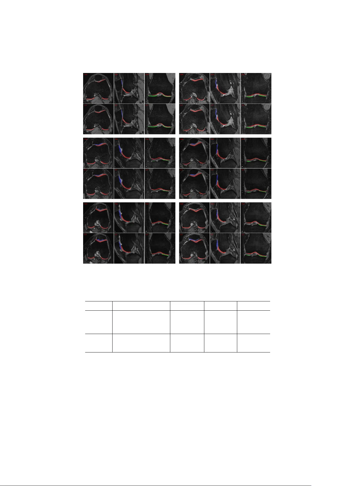
Seman tic Con text F orests for Learning-Based Knee Cartilage Segmen tation in 3D MR Images Quan W ang ?, † , Dijia W u ? , Le Lu ? , Meizh u Liu ? , Kim L. Bo yer † , and Shaoh ua Kevin Zhou ? ? Siemens Corp orate Researc h, Princeton, NJ 08540, USA † Rensselaer P olytechnic Institute, T ro y , NY 12180, USA Abstract. The automatic segmen tation of human knee cartilage from 3D MR images is a useful y et c hallenging task due to the thin sheet struc- ture of the cartilage with diffuse boundaries and inhomogeneous in tensi- ties. In this paper, we presen t an iterativ e multi-class learning method to segmen t the femoral, tibial and patellar cartilage simultaneously , which effectiv ely exploits the spatial contextual constrain ts b etw een b one and cartilage, and also b etw een different cartilages. First, based on the fact that the cartilage grows in only certain area of the corresp onding b one surface, w e extract the distance features of not only to the surface of the bone, but more informatively , to the densely registered anatomical landmarks on the b one surface. Second, we introduce a set of iterative discriminativ e classifiers that at each iteration, probability comparison features are constructed from the class confidence maps derived b y pre- viously learned classifiers. These features automatically embed the se- man tic con text information b etw een differen t cartilages of interest. V ali- dated on a total of 176 volumes from the Osteoarthritis Initiative (OAI) dataset, the prop osed approac h demonstrates high robustness and ac- curacy of segmen tation in comparison with existing state-of-the-art MR cartilage segmen tation metho ds. 1 In tro duction The quantitativ e analysis of knee cartilage is adv antageous for the study of car- tilage morphology and ph ysiology . In particular, it is an imp ortant prerequisite for the clinical assessmen t and surgical planning of the cartilage diseases, such as knee osteoarthritis which is characterized as the cartilage deterioration and a prev alen t cause of disabilit y among elderly p opulation. As the leading imaging mo dalit y used for articular cartilage quantification [ 1 ], magnetic resonance (MR) imaging provides direct and nonin v asive visualization of the whole knee joint in- cluding the soft cartilage tissues (Fig. 1c ). How ever, automatic segmentation of the cartilage tissues from MR images, which is required for accurate and repro- ducible quantitativ e cartilage measures, still remains an open problem b ecause of the inhomogeneity , small size, low tissue contrast, and shap e irregularit y of the cartilage. An earlier endea vor on this problem is F olkesson et al. ’s v oxel classification approac h [ 2 ], whic h runs an approximate k NN classifier on vo xel intensit y and 2 Q. W ang, D. W u, L. Lu, M. Liu, K. L. Boy er, S. K. Zhou absolute position based features. How ev er, due to the o verlap of intensit y distri- bution b etw een cartilage and other tissues such as menisci and m uscles, as well as the v ariability of the cartilage locations from scan to scan, the p erformance of this metho d is limited. More recen tly , Vincent et al. ha ve developed a knee join t segmen tation approach based on active app earance mo del (AAM), which captures the statistics of b oth ob ject shap e and image cues. Though promising results are reported in [ 3 ], the search for the initial model pose parameter can b e v ery time consuming even if a coarse to fine searching strategy is used. Giv en the strong spatial relation b et ween the cartilages and b ones in the knee joint, most proposed cartilage segmentation methods are based on a frame- w ork that each b one is segmented first in the knee joint [ 4 , 5 , 6 ], which is usually easier than direct cartilage segmentation because the b ones are muc h larger in size with more regular shap es. F ripp et al. segment the b ones based on 3D ac- tiv e shap e mo del (ASM) incorp orating the cartilage thic kness statistics, and the outer cartilage b oundary is then determined by examining the intensit y profile along the normal to the b one surface, while being constrained b y the cartilage thic kness model [ 4 ]. In Yin’s w ork [ 5 ], the volume of interest containing the b ones and cartilages is first detected using a learning-based approac h, then the b ones and cartilages are jointly segmented by solving an optimal multi-surface detec- tion problem via m ulti-column graph cuts [ 7 ]. Lee et al. emplo y a constrained branc h-and-mincut metho d with shap e priors to obtain the b one surface, and then segmen t the cartilage with MRF optimization based on lo cal shap e and ap- p earance information [ 6 ]. In spite of the differences, these approac hes all require classification of b one surface v oxels into b one cartilage in terface (BCI) and non- BCI, which is an imp ortant intermediate step to determine the search space or imp ose prior constraint for cartilage segmentation. Therefore, any classification error of BCI will probably propagate to the final cartilage segmentation result. In this pap er, we presen t a fully automatic learning-based v oxel classification metho d for cartilage segmen tation. It also requires pre-segmentation of corre- sp onding b ones in the knee joint. How ev er, the new approach do es not rely on explicit classification of BCI. Instead, we construct distance features from each v oxel to a large num b er of anatomical landmarks on the surface of the b ones to capture the spatial relation b etw een the cartilages and bones. By remo ving the intermediate step of BCI extraction, the whole framework is simplified and classification error propagation can b e a voided. Besides the connection betw een the cartilages and b ones, strong spatial re- lation also exists among different cartilages whic h is more often o verlooked in earlier approaches. F or example, the femoral cartilage is alwa ys ab ov e the tibial cartilage and tw o cartilages touc h each other in the region where tw o b ones slide o ver each other during joint mov ements. T o utilize this constraint, w e introduce the iterative discriminative classification that at eac h iteration, the multi-class probabilit y maps obtained by previous classifiers are used to extract semantic con text features. In particular, we compare the probabilities at p ositions with random shift and compute the difference. These features, which we name as the random shift probabilit y difference (RSPD) features, are more computation- Learning-Based Knee Cartilage Segmentation 3 ally efficien t and more flexible for differen t range of con text compared to the calculation of probabilit y statistics at fixed relative p ositions [ 8 , 9 ]. 2 Review of Bone Segmentation In this w ork, w e emplo y a learning-based bone segmentation approach whic h has sho wn the efficiency and effectiveness in differen t medical image segmentation problems [ 10 , 11 ]. W e represen t the shape of a bone by a closed triangle mesh M . Giv en a num b er of training v olumes with manual b one annotations, we use the coheren t p oin t drift algorithm (CPD) [ 12 ] to find anatomical corresp ondences of the mesh p oints and thereof construct the statistical shap e models with mean shap e M [ 13 ]. As shown in Fig. 1a , the whole b one segmentation framework comprises three steps. 1. P ose Estimation: F or a volume V , the b one is first lo calized by searching for the (sub-)optimal pose parameters ( ˆ t, ˆ r , ˆ s ), i.e. , the translation, rotation and anisotropic scaling, using the marginal space learning (MSL) [ 11 ]: ( ˆ t, ˆ r , ˆ s ) ≈ (arg max t P ( t |V ) , arg max r P ( r |V , ˆ t ) , arg max s P ( s |V , ˆ t, ˆ r )) , (1) and the shap e is initialized by linearly transforming the mean shap e M . 2. Mo del Deformation: A t this stage, the shap e is rep eatedly deformed to fit the b oundary and pro jected to the v ariation subspace until conv ergence. 3. Boundary Refinement: T o further impro v e the segmen tation accuracy , w e use the random w alks algorithm [ 14 ] to refine the b one b oundary (see T able 1 and Fig. 4 for results) and emplo y the CPD algorithm to obtain anatomically equiv alen t landmarks on the refined b one surface. 3 Cartilage Classification Giv en all three knee b ones b eing segmented, w e first extract a band of interest within a maximum distance threshold from eac h of the b one surface, and only classify vo xels in the band of in terest to simplify the training and testing by remo ving irrelev ant negative v oxels. 3.1 F eature Extraction F or each v o xel with spatial co ordinate x , we construct a n umber of base features whic h can b e categorized into three subsets. In tensity F eatures include the vo xel intensit y and its gradient magnitude, resp ectiv ely: f 1 ( x ) = I ( x ), f 2 ( x ) = ||∇ I ( x ) || . Distance F eatures measure the signed Euclidean distances from eac h v oxel to different knee bone boundaries: f 3 ( x ) = d F ( x ), f 4 ( x ) = d T ( x ), f 5 ( x ) = d P ( x ), where d F is the signed distance to the femur, d T to tibia, and d P to patella. Then w e hav e their linear combinations: f 6 / 7 ( x ) = d F ( x ) ± d T ( x ) , f 8 / 9 ( x ) = d F ( x ) ± d P ( x ) . (2) 4 Q. W ang, D. W u, L. Lu, M. Liu, K. L. Boy er, S. K. Zhou These features are useful b ecause the sum features f 6 and f 8 measure whether v oxel x locates within the narrow space b etw een t wo b ones, and the difference features f 7 and f 9 measure which b one it is closer to. Fig. 3b shows how f 6 and f 7 in addition to intensit y feature f 1 separate tibial cartilage from femoral and patellar cartilages. Giv en the prior kno wledge that the cartilage can only grow in certain area on the b one surface, it is useful for the cartilage segmentation to not only kno w ho w close the vo xel is to the b one surface, but also where it is anatomically . Therefore we define the distance features to the densely registered landmarks on the b one surface as describ ed in Section 2 : f 10 ( x , ζ ) = || x − z ζ || , where z ζ is the spatial co ordinate of the ζ th landmark of all b one mesh p oints. ζ is randomly generated in training due to the great n umber of mesh p oints av ailable (Fig. 3a ). F emur DSC (%) Tibia DSC (%) Patella DSC (%) Before R W 92 . 37 ± 1 . 58 94 . 64 ± 1 . 18 92 . 07 ± 1 . 47 After R W 94 . 86 ± 1 . 85 95 . 96 ± 1 . 64 94 . 31 ± 2 . 15 T able 1: The Dice similarit y co efficient (DSC) of b one segmen tation results b e- fore and after random w alks (3-fold cross v alidation on 176 OAI volumes). Con text F eatures compare the intensit y of the curren t v oxel x and another v oxel x + u with random offset u : f 11 ( x , u ) = I ( x + u ) − I ( x ), where u is a random offset v ector. This subset of features, named as random shift in tensity difference (RSID) features in this pap er, capture the context information in differen t ranges by randomly generating a large num b er of differen t v alues of u from a uniform distribution in training. They were earlier used to solv e p ose classification [ 15 ] and k eyp oint recognition [ 16 ] problems. 3.2 Iterativ e Seman tic Con text F orests In this pap er, w e presen t a multi-pass iterative classification metho d to automat- ically exploit the semantic context for multiple ob ject segmen tation problems. In each pass, the generated probability maps will b e used to extract the con- text em b edded features to enhance the class ification p erformance of the next pass. Fig. 1d shows a 2-pass iterative classification framework with the random forests [ 15 , 16 , 17 , 18 , 19 , 20 ] selected as the base classifier for each pass. How ev er, the metho d can b e extended to more iterations with the use of other discrimi- nativ e classifiers. Seman tic Context F eatures After each pass of the classification, the prob- abilit y maps are generated and used to extract seman tic context features as defined b elow: f 12 ( x ) = P F ( x ), f 13 ( x ) = P T ( x ), f 14 ( x ) = P P ( x ), where P F , P T and P P stand for the femoral, tibia and patellar cartilage probability map, re- sp ectiv ely . In the same fashion as the RSID features, w e compare the probabilit y resp onse of t wo vo xels with random shift: f 15 / 16 / 17 ( x , u ) = P F /T /P ( x + u ) − P F /T /P ( x ) , (3) Learning-Based Knee Cartilage Segmentation 5 CPD  I n it ia l s e g m e n t a t io n R e f in e d s e g m e n t a t io n A c t iv e s ha p e m o d e l s : • M e a n s ha p e • Sha p e v a r ia t io n s p a c e PCA  Random walks  T r a in in g v o l u m e s w it h manually annotate d bone s  C o r r e s p o n d e n c e m e s he s T r a in in g T e s t in g v o l u m e s Po s e e s ti m a ti o n b y marginal space learning  Model deformation by iterative boundary fitting  E s t im a t e d t r a n s l a t io n , r o t a t io n a n d s c a l in g Detecting ( ! , ! , ! ) ! (a) (b) (c) …… …… First pass forest Second pass forest Training imag e First pass prob. map Second pass prob. map T esting image First pass prob. map Second pass prob. map Cartilage ground truth Training Testing (d) Fig. 1: (a) The b one segmentation framework. (b) 3D anatom y of knee joint. (c) Example of a 2D MR slice [ 6 ]. (d) The semantic con text forests diagram. (a) (b) (c) (d) Fig. 2: Probability maps of femoral cartilage b y semantic context forests. (a) Original image. (b) Prob. map of the 1st pass. (c) Prob. map of the 2nd pass. (d) Ground truth. whic h is called random shift probabilit y difference features (RSPD). RSPD pro- vides semantic context information because the probability map v alues are di- rectly asso ciated with anatomical lab els, rather than original intensit y volume. In Fig. 2 , it can b e observ ed that the probabilit y map of the second pass classification is significantly enhanced with muc h less noisy resp onses, compared with the first pass. 6 Q. W ang, D. W u, L. Lu, M. Liu, K. L. Boy er, S. K. Zhou Target voxel Bone landma r ks (a) −35 −30 −25 −20 −15 −10 −5 0 5 −25 −20 −15 −10 −5 0 5 10 15 20 25 0 100 200 300 400 d F + d T d F − d T intensity Femoral cartilage Tibial cartilage Patellar cartilage Background (b) 0%# 5%# 10%# 15%# 20%# 25%# 30%# Frequency of use of different features (c) 1−pass, no LM 1−pass 2−pass, no LM 2−pass 3−pass 2−pass+GraphCuts 0.65 0.7 0.75 0.8 0.85 Femoral cartilage Tibial cartilage Patellar cartilage (d) Fig. 3: (a) Distances to densely registered bone landmarks enco de anatomical p o- sition of a vo xel. (b) F eature scatter plot: in tensity and distance features separate tibial cartilage from femoral and patellar cartilages. (c) F requency of each fea- ture selected by the classifier in the 2nd pass. (d) A comparison of segmentation p erformance (DSC): 1-pass/2-pass forests without using distance to landmark (LM) features; 1-pass/2-pass/3-pass forests using distance to landmark features; 2-pass forests with graph cuts optimization (3-fold cross v alidation). 3.3 P ost-pro cessing b y Graph Cuts Optimization After the classification, we finally use the probabilities of b eing the background and the three cartilages to construct the energy functions and p erform multi- lab el graph cuts [ 21 ] to refine the segmentation with smo othness constraints. The graph cuts algorithm assigns a lab el l ( x ) to each vo xel x , such that the energy b elo w is minimized: E ( L ) = X { x , y }∈N V x , y ( l ( x ) , l ( y )) + X x D x ( l ( x )) , (4) where L is the global lab el configuration, N is the neighborho o d system, V x , y ( · ) is the smo othness energy , and D x ( · ) is the data energy . W e define D x ( l ( x )) = − λ ln P l ( x ) ( x ) , (5) V x , y ( l ( x ) , l ( y )) = δ l ( x ) 6 = l ( y ) e ( I ( x ) − I ( y )) 2 2 σ 2 . (6) Learning-Based Knee Cartilage Segmentation 7 δ l ( x ) 6 = l ( y ) tak es v alue 1 when l ( x ) and l ( y ) are differen t lab els, and takes v alue 0 when l ( x ) = l ( y ). P l ( x ) ( x ) takes the v alue P F ( x ), P T ( x ), P P ( x ) or 1 − P F ( x ) − P T ( x ) − P P ( x ), depending on the lab el l ( x ). λ and σ are tw o parameters. λ spec- ifies the w eigh t of data energy v ersus smo othness energy , while σ is associated with the image noise [ 22 ]. 4 Exp erimen tal Results 4.1 Dataset and Exp eriment Settings The dataset we use in our work is the publicly av ailable Osteoarthritis Initiative (O AI) dataset, which contains b oth 3D MR images and ground truth cartilage annotations, referred to as “kMRI segmentations (iMorphics)”. The sagittal 3D 3T (T esla) DESS (dual echo steady state) WE (water-excitation) MR images in O AI hav e high-resolution, go o d delineation of articular cartilage, fast acquisition time and high SNR. Our dataset consists of 176 volumes from 88 sub jects, and b elongs to the Progression sub cohort, where all sub jects s ho w symptoms of OA. Eac h sub ject has tw o volumes scanned in different years. The size of each image v olume is 384 × 384 × 160 v oxels, and the vo xel size is 0 . 365 × 0 . 365 × 0 . 7 mm 3 . F or the v alidation, we divide the OAI dataset to three equally-sized subsets: D 1 , D 2 and D 3 , and p erform a three-fold v alidation. The tw o volumes from the same sub ject are alw a ys placed in the same subset. F or eac h randomized decision tree, we set the depth of the tree to 18, and train 60 trees in each pass. During training, the num b er of candidates at each non-leaf node is set to 1000. The dice similarit y co efficient (DSC) is used to measure the p erformance of our metho d since it is commonly rep orted in previous literature [ 2 , 4 , 5 , 6 , 23 ]. 4.2 Results First, we compare the frequency of different features that is selected by the classifiers. As sho wn in Fig. 3c , RSID, RSPD and the distance to dense landmarks are v ery informative features to embed spatial constraints. Then we compare the segmen tation performance with and without the use of the distance features to the anatomical dense landmarks, and also the results with different num b er of classification iterations. The results in Fig. 3d demon- strate the effectiveness of the distance features to dense landmarks and iterative classification with semantic context forests. In particular, 2-pass random forests ac hieve significan t p erformance improv emen t, whereas the gain seems quite neg- ligible b y adding more passes. Finally , the quan titative results (2-pass classification) are listed in T able 2 together with the n um b ers reported in the earlier literature. Because the datasets used are different by all these approaches, the num b ers in the table are only for reference. Note that only our exp e rimen ts are based on a relativ ely large dataset. As shown in the table, we achiev ed high p erformance with regard to the femoral and tibial cartilage, whereas the DSC of patellar cartilage is notably low er than the other tw o cartilages. This is partly b ecause the size of patellar cartilage 8 Q. W ang, D. W u, L. Lu, M. Liu, K. L. Boy er, S. K. Zhou is m uc h smaller than femoral and tibial cartilage, so that the same amount of segmen tation error will result in low er DSC. Besides, some patellar cartilage annotations in the dataset do not app ear very consistent with others. Example segmen tation results are shown in Fig. 5 . Fig. 4: Example b one segmentations. Eac h case has three views, from left to righ t: transversal plane, sagittal plane, coronal plane. Red: femur; green: tibia; blue: patella. 5 Conclusion W e hav e presented a new approach to segment the three knee cartilages in 3-D MR images, which effectively exploits the semantic context information in the knee join t. By using the distance features to the b one surface as well as to the dense anatomical landmarks on the b one surface, the spatial constrain ts betw een cartilages and b ones are incorp orated without the need of explicit extraction of the b one cartilage interface. F urthermore, the use of multi-pass iterativ e classi- fication with semantic context forests provides more spatial constraints b etw een differen t cartilages to further improv e the segmen tation. The exp eriment v ali- dation sho ws the effectiveness of this metho d. Ongoing work include the joint b one-and-cartilage v oxel classification in the iterative classification framework. References 1. Graic hen, H., Eisenhart-Rothe, R., V ogl, T., Englmeier, K.H., Eckstein, F.: Quan- titativ e assessment of cartilage status in osteoarthritis by quantitativ e magnetic resonance imaging. Arthritis Rheumatism (2004) 2. F olkesson, J., Dam, E., Olsen, O., P ettersen, P ., Christiansen, C.: Segmen ting articular cartilage automatically using a v oxel classification approac h. IEEE T rans. Med. Imag. 26 (1) (Jan. 2007) 106–115 Learning-Based Knee Cartilage Segmentation 9 Fig. 5: Examples cartilage segmen tations compared with ground truth. Eac h case has six images: segmentation results in upp er row, ground truth in low er ro w. Red: femoral cartilage; green: tibial cartilage; blue: patellar cartilage. F em. Cart. DSC Tib. Cart. DSC P at. Cart. DSC Author Dataset Mean Std. Mean Std. Mean Std. Shan [ 23 ] 18 SPGR images 78.2% 5.2% 82.6% 3.8% – – F olkesson [ 2 ] 139 Esaote C-Span images 77% 8.0% 81% 6.0% – – F ripp [ 4 ] 20 FS SPGR images 84.8% 7.6% 82.6% 8.3% 83.3% 13.5% Lee [ 6 ] 10 images in OAI 82.5% – 80.8% – 82.1% – Yin [ 5 ] 60 images in OAI 84% 4% 80% 4% 80% 4% OAI, D 1 subset (58 images) 85.47% 3.10% 84.96% 3.82% 78.56% 9.38% Proposed OAI, D 2 subset (58 images) 85.20% 3.65% 83.52% 4.08% 80.79% 7.40% method OAI, D 3 subset (60 images) 84.22% 3.05% 82.74% 3.84% 78.12% 9.63% OAI, overall (176 images) 84.96% 3.30% 83.74% 4.00% 79.16% 8.88% T able 2: Performance of our metho d compared with other state-of-the-art carti- lage segmen tation metho ds: mean DSC and standard deviation. 10 Q. W ang, D. W u, L. Lu, M. Liu, K. L. Boy er, S. K. Zhou 3. Vincen t, G., W olstenholme, C., Scott, I., Bo wes, M.: F ully automatic segmen tation of the knee joint using active app earance mo dels. In: Medical Image Analysis for the Clinic: A Grand Challenge. (2010) 4. F ripp, J., Crozier, S., W arfield, S., Ourselin, S.: Automatic segmentation and quan titative analysis of the articular cartilages from magnetic resonance images of the knee. IEEE T rans. Med. Imag. 29 (1) (Jan. 2010) 55–64 5. Yin, Y., Zhang, X., Williams, R., W u, X., Anderson, D., Sonk a, M.: Logismos – la yered optimal graph image segmentation of multiple ob jects and surfaces: Carti- lage segmentation in the knee joint. IEEE T rans. Med. Imag. 29 (12) (Dec. 2010) 2023–2037 6. Lee, S., Park, S.H., Shim, H., Y un, I.D., Lee, S.U.: Optimization of lo cal shap e and appearance probabilities for segmentation of knee cartilage in 3-d mr images. CVIU 115 (12) (Dec. 2011) 1710–1720 7. Li, K ., W u, X., Chen, D., Sonk a, M.: Optimal surface segmentation in volumetric images–a graph-theoretic approac h. IEEE T rans. P AMI 28 (1) (Jan. 2006) 119–134 8. T u, Z., Bai, X.: Auto-con text and its application to high-level vision tasks and 3d brain image segmen tation. IEEE T rans. P AMI (Oct. 2010) 1744–1757 9. Mon tillo, A., Shotton, J., Winn, J., Iglesias, J., Metaxas, D., Criminisi, A.: Entan- gled decision forests and their application for semantic segmentation of ct images. In: IPMI. (2011) 184–196 10. Ling, H., Zheng, Y., Georgescu, B., Zhou, S.K., Suehling, M.: Hierarc hical learning- based automatic liv er segmentation. In: CVPR. (2008) 11. Zheng, Y., Barbu, A., Georgescu, M., Sc heuring, M., Comaniciu, D.: F our-cham b er heart mo deling and automatic segmentation for 3D cardiac CT volumes using marginal space learning and steerable features. IEEE T rans. Med. Imag. 27 (11) (2008) 1668–1681 12. Myronenk o, A., Song, X.: Poin t set registration: Coheren t point drift. IEEE T rans. P AMI 32 (12) (Dec. 2010) 2262–2275 13. Co otes, T., T a ylor, C., Coop er, D., Graham, J.: Active shape models–their training and application. CVIU 61 (1) (1995) 38–59 14. Grady , L.: Random w alks for image segmentation. IEEE T rans. P AMI 28 (11) (No v. 2006) 1768–1783 15. Shotton, J., Fitzgibb on, A., Co ok, M., Sharp, T., Fino cchio, M., Mo ore, R., Kip- man, A., Blake, A.: Real-time human p ose recognition in parts from single depth images. In: CVPR. (Jun. 2011) 1297–1304 16. Lep etit, V., Lagger, P ., F ua, P .: Randomized trees for real-time keypoint recogni- tion. In: CVPR. V olume 2. (Jun. 2005) 775–781 vol. 2 17. Quinlan, J.R.: Induction of decision trees. Machine learning 1 (1) (1986) 81–106 18. Breiman, L.: Random forests. Machine learning 45 (1) (2001) 5–32 19. W ang, Q., Ou, Y., Julius, A.A., Bo yer, K.L., Kim, M.J.: T racking T etr ahymena Pyriformis Cells using Decision T rees. In: ICPR. (No v. 2012) 20. Zikic, D., Glo ck er, B., Konuk oglu, E., Shotton, J., Criminisi, A., Y e, D., Demiralp, C., Thomas, O., Das, T., Jena, R., et al.: Context-sensitiv e classification forests for segmen tation of brain tumor tissues, MICCAI (2012) 21. Bo yko v, Y., V eksler, O., Zabih, R.: F ast approximate energy minimization via graph cuts. IEEE T rans. P AMI 23 (11) (Nov. 2001) 1222–1239 22. Bo yko v, Y., F unk a-Lea, G.: Graph cuts and efficient n-d image segmentation. In t. J. Comput. Vis. 70 (2) (Nov. 2006) 109–131 23. Shan, L., Charles, C., Niethammer, M.: Automatic atlas-based three-lab el cartilage segmen tation from mr knee images. In: 2012 IEEE W orkshop on Mathematical Metho ds in Biomedical Image Analysis. (Jan. 2012) 241–246