PROSE: Perceptual Risk Optimization for Speech Enhancement

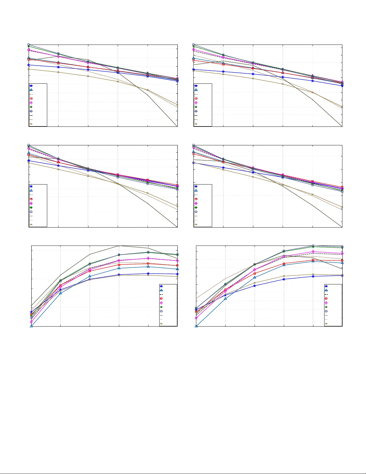
1 PR OSE: Perceptual Risk Optimization for Speech Enhancement Jishnu Sadasi v an, Chandra Sekhar Seelamantula, Senior Member , IEEE , and Nagarjuna Reddy Muraka Abstract —The goal in speech enhancement is to obtain an estimate of clean speech starting from the noisy signal by minimizing a chosen distortion measure, which r esults in an estimate that depends on the unknown clean signal or its statistics. Since access to such prior knowledge is limited or not possible in practice, one has to estimate the clean signal statistics. In this paper , we develop a new risk minimization framework for speech enhancement, in which, one optimizes an unbiased estimate of the distortion/risk instead of the actual risk. The estimated risk is expressed solely as a function of the noisy obser vations. W e consider several per ceptually rele vant distortion measures and dev elop corresponding unbiased estimates under realistic assumptions on the noise distrib ution and a priori signal-to-noise ratio (SNR). Minimizing the risk estimates gives rise to the corresponding denoisers, which are nonlinear functions of the a posteriori SNR. Perceptual evaluation of speech quality (PESQ), a verage segmental SNR (SSNR) computations, and listening tests show that the proposed risk optimization appr oach employing Itakura-Saito and weighted hyperbolic cosine distortions gives better perf ormance than the other distortion measures. F or SNRs greater than 5 dB, the proposed approach gives superior denoising performance over the benchmark techniques based on the Wiener ﬁlter , log-MMSE minimization, and Bayesian nonnegati ve matrix factorization. Index T erms — Speech enhancement, per ceptual distortion measur e, unbiased risk estimation, Stein’ s lemma, objective and subjective assessment. I . I N T R O D U C T I O N T HE goal in speech enhancement is to suppress noise and enhance signal intelligibility and quality . Over the past few decades, several techniques have been de veloped for noise suppression. The challenges are nonstationarity of the speech signal, distrib ution of noise, type of noise distortion, noise being signal-dependent or independent, etc. The problem continues to be of signiﬁcant interest to the speech community particularly considering the enormous increase in the number of smartphone users. An early revie w of v arious noise reduction techniques was giv en by Lim and Oppenheim [1]. Loizou’ s book on speech enhancement [2] is a recent and comprehensi ve reference on the topic. W e shall brieﬂy re vie w related literature before proceeding with the de velopment of the new risk optimization framework for speech enhancement. J. Sadasiv an is with the Department of Electrical Communication Engi- neering, Indian Institute of Science (IISc.), Bangalore, India; E-mail: sadasi- van@iisc.ac.in. N. R. Muraka is currently with the Indian Railways; Email: nagarjunareddy100@gmail.com. C. S. Seelamantula is with the Department of Electrical Engineering, IISc., Bangalore-560012; Email: chandra.sekhar@ieee.or g. Phone: +91 80 2293 2695. Fax: +91 80 2360 0444. The ﬁgures in this manuscript are in color in the electronic v ersion. A. Related Literatur e Speech enhancement techniques can be classiﬁed as follows. 1) Spectral subtraction algorithms: Boll [3] and W eiss et al. [4] proposed to subtract an estimate of the noise po wer spectrum from the noisy signal spectrum, in order to estimate the clean signal spectrum. The assumption is that the noise is additi ve and stationary . The noisy signal phase is used in reconstructing the time-domain signal. W eiss et al. [4] also proposed subtraction techniques in autocorrelation and cepstral domains. Lockwood and Boudy [5], Kamath and Loizou [6] proposed improved versions of spectral subtraction algorithms. 2) W iener ﬁltering tec hniques: These are based on the min- imum mean-squared error (MMSE) criterion [2], in which one constructs the W iener ﬁlter using an estimate of the clean and noisy speech power spectra. Lim and Oppenheim [1] proposed a parametric W iener ﬁlter , which allo ws for controlling the trade-of f between the signal distortion and residual noise. Hu and Loizou incorporated psychoacoustic constraints into this framework [7], [8]. In [7], the y use a perceptual weighting ﬁlter to shape the residual noise to make it inaudible. In [8], the y constrain the noise spectrum to lie belo w a preset threshold at each frequenc y . Chen et al. [9] quantiﬁed the amount of noise reduction and analyzed its relation to speech distortion. The Wiener ﬁlter requires an estimate of the a priori signal-to-noise ratio (SNR). Scalart and Filho [10] used a recursi ve a priori SNR estimator whereas Lim and Oppenheim [11] iterati vely estimated the Wiener ﬁlter based on autoregressiv e modeling of the speech signal. Hansen and Clements [12] imposed inter - and intra-frame constraints to ensure speech-like characteristics within each iteration. Sreeniv as and Kirnapure [13] proposed a codebook constrained, iterati ve W iener ﬁlter with superior conv ergence behavior . Srini vasan et al. [14], [15] proposed maximum-likelihood and Bayesian methods for estimating the speech and noise power spectra. Rosenkranz and Puder [16] proposed adaptation techniques to improve the perfor- mance of the codebook approaches reported in [14], [15] against model mismatches and unknown noise types. 3) Subspace tec hniques: Originally proposed by Ephraim and V an Trees, subspace techniques rely on eigenv alue decomposi- tion of the data covariance matrix [17]–[20] or singular-value decomposition of the data matrix [21]–[23]. The noise eigen- values/singular v alues are smaller than those of the noisy signal and denoising happens when the signal is reconstructed from the eigen/singular vectors corresponding to the signal subspace alone. Jabloun and Champagne [24] incorporated properties of human audition into the signal subspace approaches. 2 4) Statistical model based methods: McAulay and Mal- pass [25] proposed a maximum-likelihood (ML) estimator of the clean speech short-time F ourier transform (STFT) magnitude. The clean speech spectra are assumed to be deterministic and the noise is modeled as zero-mean complex Gaussian. The ML estimate of the magnitude spectrum is combined with the noisy phase spectrum in order to reconstruct the speech signal. Ephraim and Malah [26] proposed a Bayesian MMSE estimator of the short- time spectral amplitude (STSA) by assuming speech and noise to be statistically independent, zero-mean, complex Gaussian random variables. McCallum and Guillemin [27] proposed an MMSE-STSA estimator assuming a nonzero-mean speech signal. Ephraim [28] used hidden Markov model (HMMs) to model the dynamics of speech and noise processes. Erkelens et al. [29] proposed MMSE estimators of clean speech discrete Fourier transform (DFT) coefﬁcients and DFT magnitudes assuming generalized Gamma distributions on speech. Kundu et al. [30] dev eloped an MMSE estimator by using a Gaussian mixture model (GMM) for the clean speech signal. Lotter and V ary [31] proposed a maximum a posteriori (MAP) estimator assuming super-Gaussian statistics. Ephraim and Malah [32] proposed an estimator that minimizes the MSE of log-magnitude spectra as it is perceptually more correlated. Loizou [33] computed Bayesian estimators for magnitude spectrum using perceptual distortion metrics such as the Itakura-Saito distortion, hyperbolic-cosine distortion, etc. Mohammadiha et al. [34] use a Bayesian non- negati ve matrix factorization (NMF) approach to obtain an MMSE estimate of the the clean speech DFT magnitude. B. Our Contributions W e introduce the notion of risk estimation for speech denoising. The clean speech signal is considered to be deterministic and the random noise to be additive (Section II). Direct minimization of the risk results in estimates that are a function of the deterministic clean speech signal. Considering a transform-domain Gaussian observation model, one can de velop an unbiased estimate of the MSE based on Stein’ s lemma [35], which is referred to as Stein’ s unbiased risk estimator (SURE) in the literature [36], [37]. The main advantage is that, unlike MSE, SURE does not require knowledge of the unkno wn deterministic clean signal. The state- of-the-art image denoising techniques are based on risk minimiza- tion [36], [37] considering the MSE. In this paper , we solve the speech denoising problem within the frame work of unbiased risk estimation, where we derive unbiased estimates of speech-speciﬁc perceptual distortion measures and minimize them to obtain the corresponding shrinkage functions. Distortion measures such as Itakura-Saito, hyperbolic-cosine (cosh), weighted cosh, etc. are considered as they are more perceptually rele v ant than MSE [38]. Further , in practice, real-world disturbances generate bounded noise amplitudes and quantization limits the dynamic range. Therefore, we consider the more realistic case of a truncated Gaussian distribution for the samples. The details will be de- scribed in Section II. In order to dev elop a risk estimator , we make use of Stein’ s lemma and its higher-order generalization, originally proposed for Gaussian noise (Section III). The higher - order generalization becomes important in the context of percep- tual distortion measures. Correspondingly , we de velop the notion of per ceptual risk optimization for speech enhancement (PR OSE) (Section IV). The key adv antage of the PR OSE frame work is that it allows one to replace an ensemble-a veraged distortion measure by a practically viable surrogate. W e employ a transform-domain point-wise shrinkag e , which is nonlinear in the observations. W e also consider parametric versions, which gi ve additional ﬂe xibility to trade-off between residual noise le vel and speech distortion. It turns out that perceptually optimized denoising functions result in more noise attenuation than MSE. W e also carry out objecti ve assessment in terms of average segmental signal-to-noise ratio (SSNR), global SNR, perceptual ev aluation of speech quality (PESQ) [39], short-time objecti ve intelligibility (STOI) [40], and subjectiv e assessment by means of listening tests and scoring as per ITU-T recommendations [41] (Section VI). I I . P R O B L E M F O R M U L A T I O N Consider a short-time frame of noisy speech in which samples of clean speech s n are distorted additiv ely by noise w n resulting in the observations: x n = s n + w n , n = 1 , 2 , · · · , N , (1) where N is the frame length. The signal samples { s n } are assumed to be deterministic and noise samples { w n } to be zero- mean, bounded, i.i.d. random variables. Most real-world noise processes are bounded and the presence of a quantizer in a practical data acquisition scenario further justiﬁes the assumption. Consequently , { x n } are bounded, and E { x n } = s n , which implies that { x n } are independent, but not identically distributed. The time-domain noise distribution is not restricted to be a Gaussian. T ypical speech enhancement approaches work on the DFT magnitudes [2], and the phase is left unaltered. W e prefer the discrete cosine transform (DCT) as it is real-valued and known to give rise to a more parsimonious representation than the DFT [42]. Further , Soon et al. established that, for shrinkage estimators, DCT -domain denoising is superior to DFT [42]. Since our point- wise multiplicativ e shrinkage estimator belongs to this class, we prefer the DCT to DFT . The DCT representation of (1) is X k = S k + W k , k = 1 , 2 , · · · , N , (2) where the transform-domain noise { W k } being a linear combi- nation of i.i.d. random variables { w n } has a distribution that approaches a Gaussian by virtue of the central limit theor em . Howe ver , since { w n } are bounded, { W k } will also be bounded. These two properties taken together make a truncated Gaussian distribution model more appropriate and realistic for the transform coefﬁcients than the standard Gaussian. The noisy samples are concentrated about the mean and the de viations from the mean are bounded. The suitability of the truncated Gaussian for modeling real-world processes has been advocated by Burkardt [43]. The goal is to estimate S k giv en X k and noise statistics. Let 3 W indowing and orthonormal transformation Risk optimized shrinkage Inverse transformation Overlap-add synthesis Enhanced speech Noisy speech Fig. 1. A block diagram representation of the PROSE methodology . d ( S k , b S k ) denote a distortion measure that quantiﬁes the de viation of the estimate b S k from S k . The corresponding ensemble av eraged distortion or risk , as referred to in the statistics literature, is deﬁned as R = E n d ( S k , b S k ) o , where E denotes the expectation operator . The estimate is expressed as ˆ S k = f ( X k ) , where f is the denoising function , which may not always be linear . W e consider point-wise shrinkage, f ( X k ) = a k X k , a k ∈ [0 , 1] , and optimize an estimate of R with respect to a k . A block diagram representation of the proposed method is shown in Figure 1. T o take into account the quasi-stationarity of speech, denoising is performed on a frame-by-frame basis and the enhanced speech is reconstructed using the standard overlap- add synthesis methodology . I I I . R I S K E S T I M A T I O N R E S U LT S W e recall a key result from [35], which is central to the subsequent dev elopments Lemma 1: (Stein, 1981) Let W be a N (0 , σ 2 ) real random variable and let f : R → R be an indeﬁnite integral of the Lebesgue measurable function f (1) , essentially the deri v ati ve of f . Suppose also that E {| f (1) ( W ) |} < ∞ . Then, E { W f ( W ) } = σ 2 E { f (1) ( W ) } . Stein’ s lemma facilitates estimation of the mean of W f ( W ) in terms of f (1) ( W ) . Ef fectively , σ 2 f (1) ( W ) could be used as an unbiased estimate of E { W f ( W ) } . The implications of this apparently simple result can be appreciated when we are required to compute an unbiased estimator of the MSE. Next, we dev elop a higher-order generalization of Stein’ s lemma. Lemma 2: ( Generalized Stein’ s lemma ) Let W be a N (0 , σ 2 ) real random variable and let f : R → R be an n -fold indeﬁnite in- tegral of the Lebesgue measurable function f ( n ) , which is the n th deriv ativ e of f . Suppose also that E  | W ( n +1 − k ) f ( k ) ( W ) |  < ∞ , k = 1 , 2 , · · · , n . Then E { W n +1 f ( W ) } = σ 2 E { f (1) ( W ) W n } + σ 2 n E { f ( W ) W n − 1 } . Pr oof: Let us express E { W n +1 f ( W ) } as E { W g ( W ) } , where g ( W ) = W n f ( W ) . Applying Stein’ s lemma to E { W g ( W ) } , we get that E { W n +1 f ( W ) } = E { W g ( W ) } = σ 2 E { g (1) ( W ) } , = σ 2 E { f (1) ( W ) W n } + σ 2 n E { f ( W ) W n − 1 } . Stein’ s lemma could be applied recursively to each of the terms on the right-hand side, up to a stage where the terms comprise only the deriv ativ es of all orders of f up to n . Our next set of results is in the conte xt of developing Stein-type lemmas for the practical case of a truncated Gaussian distrib ution. Lemma 3: Let W be a real random variable with probability density function (p.d.f.) p ( w ; c, σ ) = 1 √ 2 π σ K exp  − w 2 2 σ 2  1 { w< | cσ |} , (3) where K ensures that p integrates to unity , c ∈ R + , and 1 denotes the indicator function. Let f : R → R be an indeﬁnite integral of the Lebesgue measurable function f (1) . Suppose also that E {| f (1) ( W ) |} < ∞ and f does not grow faster than an ex- ponential, then E { W f ( W ) } = σ 2 E { f (1) ( W ) } + O { exp( − c 2 ) } . Pr oof: Using the property: − σ 2 d exp  − w 2 2 σ 2  d w = w exp  − w 2 2 σ 2  , we write E { W f ( W ) } = Z + ∞ −∞ w f ( w ) p ( w ; c, σ ) d w , = − Z + cσ − cσ σ 2 f ( w ) 1 √ 2 π σ K d exp  − w 2 2 σ 2  d w d w , = − σ 2 f ( w ) p ( w ; c, σ )    + cσ − cσ + Z + cσ − cσ σ 2 f (1) ( w ) p ( w ; c, σ ) d w = O{ exp( − c 2 ) } + σ 2 E n f (1) ( W ) o . For even f , the approximation error is zero. Next, we state the counterpart of Lemma 2 for truncated Gaussian distribution, which has a similar proof mechanism. Lemma 4: Let W be a real random variable with p.d.f p ( w ; c, σ ) and let f : R → R be an n -fold indeﬁnite integral of the Lebesgue measurable function f ( n ) , which is the n th deriv ativ e of f . Suppose also that E  | W ( n +1 − k ) f ( k ) ( W ) |  < ∞ , k = 1 , 2 , · · · , n and f ( k ) does not grow faster than an exponential, then E { W n +1 f ( W ) } = σ 2 E { f (1) ( W ) W n } + σ 2 n E { f ( W ) W n − 1 } + O { exp( − c 2 ) } . The approximation error is ne gligible for lar ge v alues of c . These results will be handy in computing risk estimators for various perceptual distortion measures. 4 I V . P E R C E P T UA L R I S K O P T I M I Z AT I O N F O R S P E E C H E N H A N C E M E N T ( P RO S E ) A. Mean-Squar e Err or (MSE) The squared error is the most commonly employed distortion measure largely because of ease of optimization. The distortion function for squared error in the transform domain is d ( S k , b S k ) =  b S k − S k  2 , where b S k = f ( X k ) . The MSE is R = E { d ( S k , b S k ) } , which may be expanded as R = E  f 2 ( X k ) + S 2 k − 2 f ( X k ) X k + 2 f ( X k ) W k  . (4) Applying Lemma 3 giv es E { f ( X k ) W k } ≈ σ 2 E { f (1) ( X k ) } , and from (4), we get that R ≈ E { f 2 ( X k ) − 2 f ( X k ) X k + 2 σ 2 f (1) ( X k ) } + S 2 k , from which it can be concluded that b R = f 2 ( X k ) − 2 f ( X k ) X k + 2 σ 2 f (1) ( X k ) + S 2 k , (5) is a nearly unbiased estimator of the MSE. Although b R con- tains the signal term S 2 k , it does not affect the minimization with respect to f . Consider the point-wise shrinkage estimator f ( X k ) = a k X k , where a k ∈ [0 , 1] . The optimum value of a k is obtained by minimizing b R subject to the constraint a k ∈ [0 , 1] . The Karush-Kuhn-T ucker (KKT) conditions [44, pp. 211] for solving this problem are gi ven in Appendix A (cf. (25a) – (25e)). The optimum a k that satisﬁes the KKT conditions 1 is giv en by a k = max  1 − σ 2 X 2 k , 0  . The optimum shrinkage estimator becomes: b S k = max  1 − 1 ξ k , 0  X k = a MSE ( ξ k ) X k , where ξ k = X 2 k σ 2 denotes the a posteriori SNR determined based on the noisy signal, and a MSE ( ξ k ) denotes the MSE-related shrinkage function. T o impart additional ﬂexibility , we consider parametric reﬁnements, which allo w us to trade-off between residual noise level and speech distortion. It is also useful when estimates of the noise variance may not be sufﬁciently accurate. The parametrically reﬁned version is given by b S k = max  1 − α ξ k , 0  X k , (6) where α is the parameter , akin to the over -subtraction f actor in spectral subtraction algorithms. B. W eighted Euclidean (WE) Distortion The MSE is perceptually less relev ant for speech signals since a large MSE does not always imply poor signal quality . 1 The calculations related to the constrained optimization of all the perceptual risk estimates considered in this paper are provided in the supporting document. Auditory masking effects render humans more rob ust to errors at spectral peaks than at the valle ys and are taken adv antage of in speech/audio compression. One way to introduce dif ferential weighting to spectral peaks and valle ys is to consider the weighted Euclidean (WE) distortion: d ( S k , b S k ) =  b S k − S k  2 S k , where b S k = f ( X k ) . The measure d < 0 when S k < 0 , but this is not a problem, because in that case, the cost function must be maximized and not minimized. W e shall see that the proposed methodology implicitly takes care of this aspect. Developing d , we get d ( S k , b S k ) = b S 2 k S k + S k − 2 b S k . Let us consider a high-SNR scenario, that is,    W k X k    < 1 . This ev ent occurs with probability 1 if | S k | > 2 cσ (cf. Appendix B). This condition also implies that X k and S k hav e the same sign. In this scenario, the ﬁrst term is expanded as b S 2 k S k = b S 2 k X k  1 − W k X k  − 1 = b S 2 k X k ∞ X n =0  W k X k  n , and the distortion function is rewritten as d ( S k , b S k ) = b S 2 k X k ∞ X n =0  W k X k  n + S k − 2 b S k . W e truncate the inﬁnite sum beyond the fourth-order, in order to maintain high accuracy in the calculations: d ( S k , b S k ) ≈ b S 2 k X k 4 X n =0  W k X k  n + S k − 2 b S k . Considering f ( X k ) = a k X k , we seek to minimize the risk R : R = E ( a 2 k X k 4 X n =0  W k X k  n ) + S k − 2 E { a k X k } . (7) T o proceed further , we are required to compute expectations of reciprocals of truncated Gaussian random variables, which may not always be ﬁnite. A necessary and sufﬁcient condition for the expectations to be ﬁnite is that | S k | > cσ , which is satisﬁed in the high-SNR regime. This is an added beneﬁt of working with more realistic distributions such as the truncated Gaussian. A simpliﬁcation for the expectation of the sum appearing in the ﬁrst term of (7) could be made by in voking Lemma 4 (cf. Appendix C). Consequently , we get R = a 2 k E  X k + σ 2 X k − σ 4 X 3 k + 48 σ 6 X 5 k + 360 σ 8 X 7 k − 2 X k a k  + S k . The corresponding unbiased risk estimator is obtained as b R = a 2 k  X k + σ 2 X k − σ 4 X 3 k + 48 σ 6 X 5 k + 360 σ 8 X 7 k  − 2 a k X k + S k . (8) 5 The goal is to determine a k ∈ [0 , 1] such that b R is minimized if S k > 0 and maximized if S k < 0 . Solving the KKT conditions (25a) − (25e) corresponding to these two scenarios results in the same optimum a k . The corresponding estimator is giv en by b S k =  1 + 1 ξ k − 1 ξ 2 k + 48 ξ 3 k + 360 ξ 4 k  − 1 | {z } a WE ( ξ k ) X k , where a WE ( ξ k ) is the shrinkage factor . Akin to (6), one can deﬁne parametric counterparts of a WE by replacing ξ k with ξ k /α . Figure 2(a) compares a MSE and a WE for dif ferent v alues of α . W e observe that the attenuation provided by a MSE is considerably smaller than a WE when the a posteriori SNR is greater than zero dB. This indicates that, in the high-SNR regime, minimizing the weighted Euclidean distortion results in higher noise attenuation than the MSE. As α increases, the shrinkage curves shift to the right, implying more attenuation for a giv en a posteriori SNR. C. Logarithmic Mean-Square Err or (log MSE) Since loudness perception of the peripheral auditory system is logarithmic, one could compare speech spectra by computing the MSE on a logarithmic scale. This property has been used to adv antage in vector quantization and speech coding applica- tions [38]. The log MSE between S k and b S k is giv en by d ( S k , b S k ) =  log b S k S k  2 , = (log b S k ) 2 + (log S k ) 2 − 2 log S k log b S k . (9) Recall that we consider only non-negativ e shrinkage functions for denoising, and that under the high SNR assumption both b S k and S k hav e the same sign. Consequently , the argument of the logarithm is always positiv e. The last term in (9) is rewritten as log b S k log S k = log b S k log( X k − W k ) , ( from (2) ) , = log b S k log X k + log b S k log  1 − W k X k  , = log b S k log X k − log b S k ∞ X n =1 1 n  W k X k  n . Substituting in (9), truncating the series beyond n = 4 , and considering the expectation results in R = E n (log b S k ) 2 + (log S k ) 2 − 2 log b S k log X k o + E ( 2 log b S k 4 X n =1 1 n  W k X k  n ) . For the shrinkage estimate b S k = a k X k , the risk becomes R = E  (log a k X k ) 2 + (log S k ) 2  − 2 E { log a k X k log X k } + 2 E ( 4 X n =1 log a k X k n  W k X k  n ) . 0 5 10 15 20 −120 −100 −80 −60 −40 −20 0 α =1 α =2 α =3 α =1 α =2 α =3 A POSTERIORI SNR (dB) SHRINKAGE (dB) MSE WE 0 5 10 15 20 −120 −100 −80 −60 −40 −20 0 α =1 α =2 α =3 α =1 α =2 α =3 A POSTERIORI SNR (dB) SHRINKAGE (dB) MSE log MSE (a) (b) Fig. 2. A comparison of shrinkage proﬁles: (a) MSE versus WE; and (b) MSE versus Iog MSE. The last term may be simpliﬁed as shown in Appendix D, using Lemma 4. Consequently , the unbiased risk estimator is b R =(log S k ) 2 + (log a k X k ) 2 − 2 log a k X k log X k +2  σ 2 X 2 k − 1 . 5 σ 4 X 4 k + 2 . 17 σ 6 X 6 k − 159 . 5 σ 8 X 8 k  − 2 log a k X k  0 . 5 σ 2 X 2 k − 0 . 75 σ 4 X 4 k − 10 σ 6 X 6 k − 210 σ 8 X 8 k  . (10) The optimum v alue of a k ∈ [0 , 1] obtained by solving (25a) – (25e) in this case is: a k = min  exp  0 . 5 σ 2 X 2 k − 0 . 75 σ 4 X 4 k − 10 σ 6 X 6 k − 210 σ 8 X 8 k  , 1  . The corresponding estimate of S k is giv en by b S k = min  exp  0 . 5 ξ k − 0 . 75 ξ 2 k − 10 ξ 3 k − 210 ξ 4 k  , 1  | {z } a log MSE ( ξ k ) X k . The parametrized shrinkage is given by a log MSE  ξ k α  . A compar - ison of a MSE and a log MSE is shown in Figure 2(b). At low SNRs, log MSE results in a higher attenuation than MSE. D. Itakura-Saito (IS) Distortion The IS distortion, although not symmetric, is a popular quality measure used in speech coding due to its perceptual relev ance in matching two power spectra. Here, we compute the IS distortion between the DCT coefﬁcients of the noise-free speech and its estimate considering both of them to have the same sign: d ( S k , b S k ) = b S k S k − log b S k S k − 1 . In the high-SNR scenario, the distortion measure is expanded as d ( S k , b S k ) = b S k X k  1 − W k X k  − 1 − log b S k + log S k − 1 , = b S k X k ∞ X n =0  W k X k  n − log b S k + log S k − 1 . 6 0 5 10 15 20 −120 −100 −80 −60 −40 −20 0 α =1 α =2 α =3 α =1 α =2 α =3 A POSTERIORI SNR (dB) SHRINKAGE (dB) MSE IS 0 5 10 15 20 −120 −100 −80 −60 −40 −20 0 α =1 α =2 α =3 α =1 α =2 α =3 A POSTERIORI SNR (dB) SHRINKAGE (dB) IS IS−II 0 5 10 15 20 −80 −60 −40 −20 0 α =1 α =2 α =3 α =1 α =2 α =3 A POSTERIORI SNR (dB) SHRINKAGE (dB) MSE COSH 0 5 10 15 20 −80 −60 −40 −20 0 α =1 α =2 α =3 α =1 α =2 α =3 A POSTERIORI SNR (dB) SHRINKAGE (dB) COSH WCOSH (a) (b) (c) (d) Fig. 3. A comparison of shrinkage proﬁles: (a) MSE v ersus IS; (b) IS versus IS-II; (c) MSE v ersus COSH; and (d) COSH versus WCOSH. Expressing b S k = a k X k , and truncating the series beyond n = 4 , the risk turns out to be R = 4 X n =0 E  a k W n k X n k  − E { log a k X k } + log S k − 1 . (11) The ﬁrst term is ev aluated using Lemma 4 (cf. Appendix E) resulting in the risk R = E  a k  1 + 60 σ 6 X 6 k + 840 σ 8 X 8 k  − log a k X k  + log S k − 1 . The corresponding unbiased estimator of R is b R = a k  1 + 60 σ 6 X 6 k + 840 σ 8 X 8 k  − log a k X k + log S k − 1 , (12) which when optimized with respect to a k ∈ [0 , 1] (solution of (25a) to (25e)) giv es a k =  1 + 60 ξ 3 k + 840 ξ 4 k  − 1 ⇒ b S k =  1 + 60 ξ 3 k + 840 ξ 4 k  − 1 | {z } a IS ( ξ k ) X k . Figure 3(a) shows a comparison of a IS and a MSE . For a posteriori SNR greater than 0 dB, the attenuation is higher in the case of Itakura-Saito distortion. E. Itakura-Saito Distortion Between DCT P ower Spectra (IS-II) W e next consider the IS distortion between S 2 k and b S 2 k : d ( S k , b S k ) = b S 2 k S 2 k − log b S 2 k S 2 k − 1 , = b S 2 k X 2 k  1 − W k X k  − 2 − log b S 2 k + log S 2 k − 1 , = b S 2 k X 2 k ∞ X n =0 ( n + 1)  W k X k  n − log b S 2 k + log S 2 k − 1 . Considering b S k = a k X k , and truncating the series beyond n = 4 , results in the risk R = E ( a 2 k 4 X n =0 ( n + 1)  W k X k  n ) − E  log a 2 k X 2 k  + log S 2 k − 1 . Simplifying the ﬁrst term using Lemma 4 giv es R = a 2 k E  1 + σ 2 X 2 k − 3 σ 4 X 4 k + 360 σ 6 X 6 k + 4200 σ 8 X 8 k  − E  log a 2 k X 2 k  + log S 2 k − 1 . An unbiased estimator of R is b R = a 2 k  1 + σ 2 X 2 k − 3 σ 4 X 4 k + 360 σ 6 X 6 k + 4200 σ 8 X 8 k  − log a 2 k X 2 k + log S 2 k − 1 . (13) Optimizing b R with respect to a k ∈ [0 , 1] , following (25a) – (25e), we get a k = min ( 1 ,  1 + σ 2 X 2 k − 3 σ 4 X 4 k + 360 σ 6 X 6 k + 4200 σ 8 X 8 k  − 1 2 ) , ⇒ b S k = min ( 1 ,  1 + 1 ξ k − 3 ξ 2 k + 360 ξ 3 k + 4200 ξ 4 k  − 1 2 ) | {z } a IS-II ( ξ k ) X k , which we shall refer to as the IS-II estimator . A comparison of the IS and IS-II shrinkage functions is sho wn in Figure 3(b). At low SNRs, IS attenuates more than IS-II. F . Hyperbolic Cosine Distortion Measure (COSH) A symmetrized version of the IS distortion results in the cosh measure: d ( S k , b S k ) = cosh  log S k b S k  − 1 = 1 2 " S k b S k + b S k S k # − 1 . The corresponding risk is R = 1 2 E  S k b S k  + 1 2 E ( b S k S k ) − 1 . Substituting b S k = a k X k , and in voking Lemma 4, the expectations turn out to be E  S k a k X k  = E  1 a k + σ 2 a k X 2 k  , and E  a k X k S k  = E  a k  1 + 60 σ 6 X 6 k + 840 σ 8 X 8 k  . 7 Correspondingly , the unbiased risk estimator is b R = 1 2  1 a k + σ 2 a k X 2 k + a k  1 + 60 σ 6 X 6 k + 840 σ 8 X 8 k  − 1 . (14) Optimizing b R with respect to a k ∈ [0 , 1] following (25a)–(25e) giv es b S k = min          1 , v u u u u u t 1 + 1 ξ k 1 + 60 1 ξ 3 k + 840 1 ξ 4 k          | {z } a COSH ( ξ k ) X k . Figure 3(c) sho ws a comparison of a MSE and a COSH versus ξ k – it is clear that a COSH results in a higher attenuation than a MSE . G. W eighted COSH Distortion (WCOSH) Similar to the weighted Euclidean measure, we consider the weighted cosh distortion: d ( S k , b S k ) = 1 2 " S k b S k + b S k S k # − 1 ! 1 S k . (15) The risk estimator can be computed as in the case of the cosh measure (cf. Appendix F). The optimal estimate is giv en by b S k = min ( 1 ,  1 − 1 ξ k + 3 ξ 2 k + 420 ξ 3 k + 8400 ξ 4 k  − 1 2 ) | {z } a WCOSH ( ξ k ) X k . A comparison of a COSH and a WCOSH shown in Figure 3(d) indicates that the latter results in higher noise attenuation at high noise lev els. V . I M P L E M E N T A T I O N D E TA I L S For experimental validation, we use the clean speech and nonstationary noise data from the NOIZEUS database [45] ( 8 kHz sampling frequency and 16 -bit quantization). Noisy speech is generated by adding noise at a desired global SNR. The noisy speech signal is processed in the DCT domain on a frame-by- frame basis. The frame size is 40 ms, the window function is Hamming, and the overlap between consecutiv e frames is 75% . W e experiment with both stationary and nonstationary noise types. The developments in the PROSE framew ork assumed knowledge of the noise v ariance in each bin of a given frame. In practice, the noise variance has to be estimated. For this purpose, we use the likelihood-ratio-test-based voice activity detector (V AD) of Sohn et al. [46], which w as also employed in the e xtensi ve comparisons reported by Hu and Loizou [45]. The in verse a posteriori SNR is then estimated using the recursiv e formula 1 b ξ k ( i ) = β b σ 2 k ( i ) X 2 k ( i ) + (1 − β ) max 1 − b S 2 k ( i − 1) X 2 k ( i − 1) , 0 ! , (16) where k denotes the index of the DCT coef ﬁcient, i denotes the frame index, and β is a smoothing parameter (set to 0 . 98 in our experiments), b σ 2 k ( i ) is the estimate of the noise variance at the k th DCT coefﬁcient in the i th frame, b S k ( i − 1) is the denoised k th DCT coefﬁcient in the ( i − 1) th frame. The ﬁrst few frames are assumed to contain only noise. For the ﬁrst frame, β is set to unity , and the k th noise v ariance is estimated by averaging the noise variances of the k th coefﬁcient in the ﬁrst ten frames. The noise v ariance is updated in the noise-only frames as classiﬁed by the V AD following the recursion: b σ 2 k ( i ) = ( η b σ 2 k ( i − 1) + (1 − η ) X 2 k ( i ) , under H 0 , b σ 2 k ( i − 1) , under H 1 , where H 0 and H 1 are the null hypothesis (noise-only) and the alternativ e hypothesis (signal + noise), respectiv ely . The value of η = 0 . 98 follo wing [45]. The noisy speech signals are denoised using shrinkage functions corresponding to various distortion measures considered in this paper . W e set α = 1 . 75 uniformly across all measures in the PR OSE framework as it was found to gi ve better results than α = 1 . The enhanced speech frames are combined using overlap-and-add synthesis to result in the denoised speech signal. V I . E X P E R I M E N TA L R E S U LT S The denoising performance of PROSE estimators is ev aluated using both objective measures and subjectiv e listening tests. For benchmarking, we use three algorithms: (i) W iener ﬁlter method, where a priori SNR is estimated using the decision- directed approach (WFIL) [10]; (ii) a Bayesian estimator for short-time log-spectral amplitude (LSA) [32]; and (iii) Bayesian non-negati ve matrix factorization algorithm (BNMF) [34] 2 , which giv es an MMSE estimate of the clean speech DFT magnitude. In the BNMF approach, the speech bases are learned ofﬂine and the noise bases are learned online. The WFIL and LSA algorithms were sho wn to perform better than the other techniques in an extensi ve e valuation carried out by Hu and Loizou [45] 3 . In terms of intelligibility also, these techniques were shown to be superior (Ch. 11, pp. 567 of [2]). BNMF has been shown to be the best among the NMF approaches for speech enhancement. A. Objective Evaluation The denoising performance is quantiﬁed in terms of: (i) global SNR; (ii) av erage segmental SNR (SSNR), a local metric, which is the average of the SNRs computed ov er short segments; (iii) perceptual e v aluation of speech quality (PESQ) [39], which is an objectiv e score for assessing end-to-end speech quality in narrowband telephone networks and speech codecs, described in ITU-T Recommendation P .862 [39]; and (iv) short-time objecti ve 2 Matlab implementation av ailable online: https://www .uni- oldenburg.de/en/ mediphysics- acoustics/sigproc/staff/nasser- mohammadiha/matlab- codes/ 3 Matlab implementations of algorithms used in [45] are av ailable with [2]. For performance comparisons, we hav e used Matlab codes given with [2]. 8 intelligibility measure (STOI) [40] 4 , which ranges from 0 to 1 and reﬂects the correlation between short-time temporal env elope of clean speech and denoised speech. It has been shown to correlate highly with the intelligibility scores obtained through listening tests [40]. Measures (i), (ii), and (iii) assess the speech quality , whereas (i v) measures the intelligibility . For SNR, SSNR, and PESQ, we report the gains achiev ed by denoising. The SNR gain is the difference between the output and input SNR values. The PESQ gain and the SSNR gain are also computed similarly . W e consider all 30 speech ﬁles from the NOIZEUS database [45], and three noise types – white Gaussian noise, train noise, and street noise, the last two being real-world nonstationary noise types. The results presented here are obtained after averag- ing ov er the entire database for 50 noise realizations. 1) White Gaussian noise: Figure 4(a) shows the SNR gain of different algorithms in white Gaussian noise. For input SNRs in the range of − 5 dB to 20 dB, PR OSE with cosh and log-MSE distortions results in a higher SNR gain compared with the other algorithms, followed by IS and WE. As the input SNR increases, the mar gin of improvement offered by PROSE techniques over BNMF , LSA, and WFIL increases. The se gmental SNR (SSNR) gain is shown in Figure 4(b). The trends of SSNR gain and SNR gain are similar . The gains are negati ve for the competing techniques at high SNRs. A negativ e gain indicates that the output SSNR or PESQ score is worse than that of the input. The PESQ scores are shown in Figure 4(c). For input SNR in the range − 5 dB to 20 dB, the PESQ gain is maximum for WE, log MSE, and IS. Below 5 dB input SNR, BNMF also shows a high PESQ gain. W e observe that, within the PR OSE framework, PESQ gains are higher for perceptually motiv ated distortions than the MSE. The denoising performance of PROSE based on WE, log MSE, COSH, and IS distortions is better in terms of SNR, SSNR, and PESQ compared with the benchmark techniques. The ST OI scores are shown in T able I. W e observe that for SNRs belo w 5 dB, BNMF has higher STOI scores than the other algorithms. For SNRs greater than 5 dB, the PR OSE framework results in a higher STOI. 2) Str eet noise: The denoising results are presented in Fig- ure 5. The PR OSE frame work based on WCOSH, WE, IS and IS-II distortions results in a higher SNR gain and SSNR gain than the other algorithms. (cf. Figures 5(a) and (b)). Similar to the white noise scenario, the margin of impro vement in case of PR OSE increases with increase in input SNR than the benchmark algorithms. The PESQ gain shows a slightly different trend (Figure 5(c)). BNMF giv es a mar ginally higher PESQ gain (about 0.05 higher) than PR OSE. This is attributed to the training phase in BNMF , which is particularly adv antageous in lo w SNR and nonstationary noise conditions. W ithin the PROSE family of denoisers, distortion measures other than the MSE result in a higher PESQ score. T able II shows the STOI scores. W e observe that, for SNRs greater than 5 dB, PROSE algorithms yields a higher STOI score than BNMF , WFIL, and LSA. 4 Matlab implementation available at http://siplab .tudelft.nl/ −5 0 5 10 15 20 −2 0 2 4 6 8 10 INPUT SNR (dB) SNR GAIN (dB) MSE log MSE WE COSH IS IS−II WCOSH BNMF LSA WFIL (a) −5 0 5 10 15 20 −2 0 2 4 6 8 10 INPUT SNR (dB) SSNR GAIN (dB) MSE log MSE WE COSH IS IS−II WCOSH BNMF LSA WFIL (b) −5 0 5 10 15 20 0.25 0.3 0.35 0.4 0.45 0.5 0.55 0.6 0.65 0.7 INPUT SNR (dB) PESQ GAIN MSE log MSE WE COSH IS IS−II WCOSH BNMF LSA WFIL (c) Fig. 4. [Color online] Denoising performance in white Gaussian noise: (a) SNR gain; (b) SSNR gain; and (c) PESQ gain. 3) T rain noise: Figure 6 compares the denoising performance in train noise. Similar to the street noise scenario, PROSE denoisers based on WCOSH, IS-II, and WE yield a higher SNR and SSNR gain than BNMF , WFIL and LSA (cf. Figures 6(a) and (b)). Although the SNR and SSNR gain trends are similar to the street noise scenario, the margin of improvement is higher in train noise. This may be because street noise is comparativ ely more nonstationary than train noise, which may have resulted 9 −5 0 5 10 15 20 −3 −2 −1 0 1 2 3 4 5 INPUT SNR (dB) SNR GAIN (dB) MSE log MSE WE COSH IS IS−II WCOSH BNMF LSA WFIL (a) −5 0 5 10 15 20 −5 −4 −3 −2 −1 0 1 2 3 4 5 INPUT SNR (dB) SSNR GAIN (dB) MSE log MSE WE COSH IS IS−II WCOSH BNMF LSA WFIL (b) −5 0 5 10 15 20 0 0.05 0.1 0.15 0.2 0.25 0.3 0.35 INPUT SNR (dB) PESQ GAIN MSE log MSE WE COSH IS IS−II WCOSH BNMF LSA WFIL (c) Fig. 5. [Color online] A comparison of denoising performance in street noise: (a) SNR gain; (b) SSNR gain; and (c) PESQ gain. in less accurate estimates of the noise standard deviation. From Figure 6(c), we observe that for input SNRs greater than 5 dB, PR OSE denoisers with WCOSH and IS-II measures are better than all the other methods. F or input SNRs lo wer than 5 dB, LSA giv es a PESQ gain about 0.05 higher than the rest. PESQ gains are also higher in case of train noise than street noise. T able III shows the corresponding STOI scores and the trends are similar to the street noise scenario. −5 0 5 10 15 20 −3 −2 −1 0 1 2 3 4 5 6 7 INPUT SNR (dB) SNR GAIN (dB) MSE log MSE WE COSH IS IS−II WCOSH BNMF LSA WFIL (a) −5 0 5 10 15 20 −4 −2 0 2 4 6 INPUT SNR (dB) SSNR GAIN (dB) MSE log MSE WE COSH IS IS−II WCOSH BNMF LSA WFIL (b) −5 0 5 10 15 20 0 0.05 0.1 0.15 0.2 0.25 0.3 0.35 0.4 0.45 INPUT SNR (dB) PESQ GAIN MSE log MSE WE COSH IS IS−II WCOSH BNMF LSA WFIL (c) Fig. 6. [Color online] A comparison of denoising performance in train noise: (a) SNR gain; (b) SSNR gain; and (c) PESQ gain. T o summarize, the PR OSE denoisers based on WCOSH, IS- II, IS, and WE sho w consistently superior denoising performance in terms of SNR and SSNR compared with LSA, WFIL, and BNMF . The mar gin of improvement ov er LSA, WFIL, and BNMF also increases with SNR. W ithin the PR OSE family of denoisers, the PESQ gains are higher for perceptual measures than MSE. For highly nonstationary noise types such as the street noise, the BNMF technique is marginally better at lo w SNRs, which 10 T ABLE I C O M P A R I S O N O F D E N O I S I N G P E R F O R M A N C E I N T E R M S O F ST O I S C O R E S F O R D I FF E R E N T I N P U T S N R S ( W H I T E G AU S S I A N N O I S E ) . SNR (dB) − 5 0 5 10 15 20 Input 0 . 560 0 . 663 0 . 757 0 . 835 0 . 894 0 . 936 MSE 0 . 571 0 . 686 0 . 785 0 . 861 0 . 916 0 . 952 log MSE 0 . 534 0 . 659 0 . 772 0 . 863 0 . 919 0.956 WE 0 . 546 0 . 664 0 . 773 0 . 863 0.920 0.956 COSH 0 . 559 0 . 677 0 . 782 0.865 0.920 0.956 IS 0 . 543 0 . 658 0 . 767 0 . 861 0 . 919 0 . 955 IS-II 0 . 553 0 . 664 0 . 768 0 . 860 0 . 918 0 . 955 WCOSH 0 . 553 0 . 660 0 . 763 0 . 858 0 . 916 0 . 953 BNMF 0.586 0.707 0.802 0 . 864 0 . 901 0 . 923 LSA 0 . 565 0 . 664 0 . 764 0 . 843 0 . 898 0 . 939 WFIL 0 . 570 0 . 682 0 . 781 0 . 858 0 . 911 0 . 948 T ABLE II C O M P A R I S O N O F D E N O I S I N G P E R F O R M A N C E I N T E R M S O F ST O I S C O R E S F O R D I FF E R E N T I N P U T S N R S ( S T R E E T N O I S E ) . SNR (dB) − 5 0 5 10 15 20 Input 0 . 540 0 . 659 0 . 774 0 . 867 0 . 930 0 . 967 MSE 0 . 536 0 . 669 0.790 0.881 0 . 939 0.972 log MSE 0 . 512 0 . 650 0 . 778 0 . 878 0 . 939 0 . 971 WE 0 . 515 0 . 653 0 . 780 0 . 879 0.940 0.972 COSH 0 . 524 0 . 663 0 . 785 0.881 0.940 0.972 IS 0 . 510 0 . 647 0 . 775 0 . 876 0 . 939 0 . 971 IS-II 0 . 515 0 . 650 0 . 776 0 . 876 0 . 939 0 . 971 WCOSH 0 . 511 0 . 646 0 . 772 0 . 873 0 . 937 0 . 971 BNMF 0.543 0.672 0 . 786 0 . 865 0 . 910 0 . 932 LSA 0 . 512 0 . 637 0 . 757 0 . 854 0 . 921 0 . 960 WFIL 0 . 528 0 . 658 0 . 777 0 . 871 0 . 932 0 . 967 is attributed to the training process. F or SNRs belo w 0 dB, the PESQ gain offered by PR OSE is not signiﬁcant and in the case of street noise, e ven negativ e. This is due to inaccuracy in estimating noise v ariance in highly nonstationary conditions such as street noise. For input SNRs greater than 5 dB, the PROSE methodology and WFIL giv e consistently better STOI scores, unlike LSA and BNMF approaches. The entire repository of denoised speech ﬁles under v arious noise conditions is a vailable online at: http://spectrumee.wix.com/prose. B. Subjective Evaluation W e consider four speech ﬁles (two male and two female speakers) at SNRs 0, 10, and 20 dB. Fifteen listeners in the age group of 20 − 35 years endowed with normal hearing were selected for the listening test. The subjects were giv en a Sennheiser HD650 headphone for listening, and were asked to rate the enhanced speech signal based on the ITU-T recommended P .835 scale [41]: (i) Speech signal distortion (SIG); 1 : very distorted, 2 : fairly dis- torted, 3 : somewhat distorted, 4 : little distorted, 5 : not distorted; T ABLE III C O M P A R I S O N O F D E N O I S I N G P E R F O R M A N C E I N T E R M S O F ST O I S C O R E S F O R V A R I O U S I N P U T S N R S ( T R A I N N O I S E ) . SNR (dB) − 5 0 5 10 15 20 Input 0 . 554 0 . 681 0 . 796 0 . 883 0 . 942 0 . 975 MSE 0.552 0.695 0.813 0 . 896 0.949 0.978 log MSE 0 . 516 0 . 675 0 . 808 0 . 896 0 . 948 0 . 977 WE 0 . 522 0 . 678 0 . 809 0 . 897 0.949 0 . 977 COSH 0 . 536 0 . 687 0.813 0.898 0.949 0.978 IS 0 . 513 0 . 670 0 . 805 0 . 896 0 . 948 0 . 977 IS-II 0 . 521 0 . 674 0 . 806 0 . 896 0 . 948 0 . 977 WCOSH 0 . 517 0 . 667 0 . 801 0 . 893 0 . 947 0 . 976 BNMF 0 . 549 0 . 688 0 . 804 0 . 878 0 . 917 0 . 936 LSA 0 . 522 0 . 661 0 . 784 0 . 874 0 . 932 0 . 966 WFIL 0 . 538 0 . 680 0 . 799 0 . 886 0 . 942 0 . 974 (ii) Background intrusiv eness (BAK); 1 : very intrusiv e, 2 : some- what intrusiv e, 3 : noticeable but not intrusiv e, 4 : somewhat noticeable, 5 : not noticeable; and (iii) Overall quality (O VRL); 1 : bad, 2 : poor , 3 : fair , 4 : good, 5 : excellent. The listening tests were conducted in three sessions, one for each noise type (white/street/train) at all SNRs. Follo wing the ITU-T recommendation, each session is further divided into two subsessions. In the ﬁrst one, two ﬁles (one male and one female speaker) are used with the rating order as SIG − B AK − O VRL and in the second one, the other two ﬁles (again one male and one female speaker) are presented and the order of rating is BAK − SIG − O VRL. The two-session test is done to suppress listener’ s bias. In each subsession, the listeners rate the denoising performance of all the algorithms. Thus, in one subsession, a listener had to grade a total of 2 (speakers) × 3 (SNRs) × 11 (algorithms) = 66 ﬁles. The subjects were gi ven suf ﬁcient time to relax within and across subsessions, and across SNRs. The denoised speech ﬁles were presented in a random order, and the scores were derandomized accordingly before calculating the av erage scores. The listeners were gi ven a token re ward at the end of the listening test. Figure 7 shows the mean scores of SIG, B AK, and O VRL for white noise, street noise, and train noise. W e observe that, among the PROSE algorithms, WCOSH exhibits a consistently high denoising performance in terms of SIG, B AK, and O VRL scores compared with the other algorithms. Among the techniques considered for benchmarking performance, LSA sho ws a consistently higher performance. The performances of LSA and PR OSE with WCOSH are comparable. Also, PR OSE consistently improv es the BAK and O VRL scores compared with the noisy signal. Listening results reveal that, for all the algorithms considered, the extent of improvement in SIG scores is not signiﬁcant compared with the improvement in B AK and O VRL scores. Within the PR OSE family , WCOSH, IS-II, and IS show a high B AK and O VRL scores, whereas MSE results in a lower score, compared with the other algorithms. 11 SNR = 0 dB SNR = 10 dB SNR = 20 dB White noise 0 1 2 3 4 5 BNMF COSH IS−II IS LSA log MSE NOISY MSE WCOSH WFIL WE SIG BAK OVRL 0 1 2 3 4 5 BNMF COSH IS−II IS LSA log MSE NOISY MSE WCOSH WFIL WE SIG BAK OVRL 0 1 2 3 4 5 BNMF COSH IS−II IS LSA log MSE NOISY MSE WCOSH WFIL WE SIG BAK OVRL Street noise 0 1 2 3 4 5 BNMF COSH IS−II IS LSA log MSE NOISY MSE WCOSH WFIL WE SIG BAK OVRL 0 1 2 3 4 5 BNMF COSH IS−II IS LSA log MSE NOISY MSE WCOSH WFIL WE SIG BAK OVRL 0 1 2 3 4 5 BNMF COSH IS−II IS LSA log MSE NOISY MSE WCOSH WFIL WE SIG BAK OVRL T rain noise 0 1 2 3 4 5 BNMF COSH IS−II IS LSA log MSE NOISY MSE WCOSH WFIL WE SIG BAK OVRL 0 1 2 3 4 5 BNMF COSH IS−II IS LSA log MSE NOISY MSE WCOSH WFIL WE SIG BAK OVRL 0 1 2 3 4 5 BNMF COSH IS−II IS LSA log MSE NOISY MSE WCOSH WFIL WE SIG BAK OVRL Fig. 7. [Color online] A comparison of the mean v alues of SIG, BAK, and O VRL ratings of the enhanced signal. C. Spectr ograms Figure 8 shows the spectrograms of clean, noisy (SNR = 10 dB), and enhanced signals for the case of train noise. W e observe that WFIL and LSA result in signiﬁcant residual noise, whereas BNMF has relativ ely lower residual noise. BNMF recov ers clean speech spectra with less distortion in some regions, compared with other algorithms (cf. green box), b ut it introduces distortions in the other parts (highlighted by the blue box for instance). PR OSE with WCOSH results in superior noise suppression with minimal speech distortion than WFIL, LSA, and BNMF . Both PR OSE and BNMF introduce a small amount of musical noise, in particular , in the silence regions. Regions that are submerged in noise are difﬁcult to recover by any algorithm (red box, for instance), which explains why the improvements in SIG scores are lo wer than improvements in BAK and O VRL for all the techniques. V I I . C O N C L U S I O N S W e introduced the notion of unbiased risk estimation within a perceptual frame work (abbreviated PR OSE) for performing single-channel speech enhancement. The analytical developments are based on Stein’ s lemma and its generalized version introduced in this paper, which proved to be efﬁcient for obtaining unbiased estimates of the distortion measures. W e have also established the optimality of the shrinkage parameters considering the Karush- Kuhn-T ucker conditions. V alidation on sev eral speech signals in both synthesized noise and real-world nonstationary noise scenar- ios, and comparisons with benchmark techniques showed that, for input SNR greater than 5 dB, the proposed PR OSE method results in better denoising performance. W ithin the PR OSE family , estimators based on Itakura-Saito distortion and weighted cosh distortion resulted in superior denoising performance. It must be emphasized that the PR OSE methodology is relativ ely simpler from an implementation perspective (recall Fig. 1) and does not require any training, making it ideal for deployment in practical applications in volving hearing aids, mobile devices, etc. Further, we employed a voice-activity detector and a recursive algorithm for estimating the time-varying a posteriori SNR. Improving on the accuracy of noise variance estimation for handling rapidly changing noise would further enhance the performance of the PR OSE method. A C K N O W L E D G M E N T S W e would like to thank Subhadip Mukherjee for technical discussions and the subjects for participating in the listening test. W e would also like to thank Mohammadiha et al. [34] and T aal et al. [40] for providing the Matlab implementations of their algorithms online, which facilitated the comparisons. 12 Clean signal TIME (s) FREQUENCY (kHz) 0 1 2 3 4 5 6 7 0 1 2 3 4 dB 0 20 40 Noisy speech TIME (s) FREQUENCY (kHz) 0 1 2 3 4 5 6 7 0 1 2 3 4 dB 0 20 40 PR OSE (WCOSH) TIME (s) FREQUENCY (kHz) 0 1 2 3 4 5 6 7 0 1 2 3 4 dB 0 20 40 LSA TIME (s) FREQUENCY (kHz) 0 1 2 3 4 5 6 7 0 1 2 3 4 dB 0 20 40 WFIL TIME (s) FREQUENCY (kHz) 0 1 2 3 4 5 6 7 0 1 2 3 4 dB 0 20 40 BNMF TIME (s) FREQUENCY (kHz) 0 1 2 3 4 5 6 7 0 1 2 3 4 dB 0 20 40 Fig. 8. [Color online] Spectrograms of clean speech, noisy speech, and speech denoised using various approaches. The utterance is: “He knew the skill of the great young actress. Wipe the grease of f his dirty face. W e ﬁnd joy in the simplest things. ” A P P E N D I X A K A R U S H - K U H N - T U C K E R C O N D I T I O N S The goal is to solve the optimization problem min a k b R subject to a k ∈ [0 , 1] . The corresponding Lagrangian is L ( a k , λ 1 , λ 2 ) = b R + λ 1 ( a k − 1) − λ 2 a k , where λ 1 , λ 2 ∈ R + ∪ { 0 } . The KKT conditions are as follows: C1 : d L ( a k , λ 1 , λ 2 ) d a k = 0 , (17a) C2 : λ 1 ( a k − 1) = 0 , − λ 2 a k = 0 , (17b) C3 : a k ∈ [0 , 1] , (17c) C4 : λ 1 ≥ 0 , λ 2 ≥ 0 , and (17d) C5 : d 2 L ( a k , λ 1 , λ 2 ) d a 2 k > 0 . (17e) Solving (25a) − (25e) gives the optimum shrinkage parameter a k . The deri vations for all the distortion measures are provided in the supporting document. A P P E N D I X B T H E H I G H - S N R S C E N A R I O The a priori SNR is deﬁned as SNR := S k 2 σ 2 . By high SNR, we mean that SNR > 4 c 2 . Consider the probability: Prob {| W k | < | X k |} = Prob  X k 2 − W k 2 > 0  , = Prob { ( X k + W k )( X k − W k ) > 0 } , = Prob { S k ( X k + W k ) > 0 } , = Prob  W k < − S k 2  , if S k < 0 = Prob  W k > − S k 2  , if S k > 0 . (18) Therefore, Prob {| W k | < | X k |} = Prob n W k < | S k | 2 o = 1 if | S k | > 2 cσ ⇒ a priori SNR > 4 c 2 . A P P E N D I X C W E I G H T E D E U C L I D E A N D I S TA N C E Consider E ( a 2 k X k 4 X n =0  W k X k  n ) = a 2 k E  X k + W k + W 2 k X k + W 3 k X 2 k + W 4 k X 3 k  . (19) Using Lemma 4, we hav e that E  W 2 k X k  = σ 4 E  2 X 3 k  + σ 2 E  1 X k  , E  W 3 k X 2 k  = σ 6 E  − 24 X 5 k  + σ 4 E  − 6 X 3 k  , and E  W 4 k X 3 k  = σ 8 E  360 X 7 k  + σ 6 E  72 X 5 k  + 3 σ 4 E  1 X 3 k  . 13 Substituting the preceding expressions in (19), we get E ( a 2 k X k 4 X n =0  W k X k  n ) = a 2 k E  X k + σ 2 X k − σ 4 X 3 k + 48 σ 6 X 5 k + 360 σ 8 X 7 k  . A P P E N D I X D L O G M E A N - S Q U A R E E R R O R Consider E ( 4 X n =1 log a k X k n  W k X k  n ) = E ( 4 X n =1 J n ( X k ) W n k ) , where J n ( X k ) = log a k X k / ( nX n k ) . Applying Lemma 4 giv es E { J 1 ( X k ) W k } = σ 2 E { J (1) 1 ( X k ) } , E { J 2 ( X k ) W 2 k } = σ 4 E { J (2) 2 ( X k ) } + σ 2 E { J 2 ( X k ) } , E { J 3 ( X k ) W 3 k } = σ 6 E { J (3) 3 ( X k ) } + 3 σ 4 E { J (1) 3 ( X k ) } , and E { J 4 ( X k ) W 4 k } = E { σ 8 J (4) 4 ( X k ) + 6 σ 6 J (2) 4 ( X k ) + 3 σ 4 J 4 ( X k ) } , where J (1) 1 = 1 X 2 k − log a k X k X 2 k , J (2) 2 = − 5 2 X 4 k + 3 log a k X k X 4 k , J (1) 3 = 1 3 X 4 k − log a k X k X 4 k , J (3) 3 = 47 3 X 6 k − 20 log a k X k X 6 k , J (2) 4 = − 9 4 X 6 k + 5 log a k X k X 6 k , J (4) 4 = − 638 4 X 8 k + 210 log a k X k X 8 k . A P P E N D I X E I TA K U R A - S A I T O D I S T O RT I O N W ith reference to (11), consider the truncated approximation: ∞ X n =0 E { a k W n k /X n k } ≈ 4 X n =0 E { a k W n k /X n k } . (20) Applying Lemma 4, we hav e that E  W k X k  = σ 2 E  − 1 X 2 k  , E  W 2 k X 2 k  = E  σ 4 6 X 4 k + σ 2 1 X 2 k  , E  W 3 k X 3 k  = σ 6 E  − 60 X 6 k  + 3 σ 4 E  − 3 X 4 k  , and E  W 4 k X 4 k  = σ 8 E  840 X 8 k  + 6 σ 6 E  20 X 6 k  + 3 σ 4 E  1 X 4 k  . The ﬁnal expression for (20) is given by 4 X n =0 E { a k W n k /X n k } = a k E  840 σ 8 X 8 k + 60 σ 6 X 6 k + 1  . (21) A P P E N D I X F W E I G H T E D C O S H D I S T A N C E W e provide certain simpliﬁcations for the expectation terms in the risk estimator for weighted cosh measure: R = E n d ( S k , b S k ) o = 1 2 E ( 1 b S k + b S k S 2 k ) − 1 S k . (22) The second term in (22) is approximated as b S k X 2 k  1 − W k X k  − 2 ≈ b S k X 2 k  1 + 2 W k X k + 3 W 2 k X 2 k + 4 W 3 k X 3 k + 5 W 4 k X 4 k  . Substituting b S k = a k X k and taking expectation, we get that E ( b S k S 2 k ) = E  a k X k X 2 k  1 + 2 W k X k + 3 W 2 k X 2 k + 4 W 3 k X 3 k + 5 W 4 k X 4 k  . Simpliﬁed expressions for the individual terms in the abov e equation are giv en belo w: E  W k X 2 k  = σ 2 E  − 2 X 3 k  , E  W 2 k X 3 k  = E  σ 4 12 X 5 k + σ 2 1 X 3 k  , E  W 3 k X 4 k  = σ 6 E  − 120 X 7 k  + 3 σ 4 E  − 4 X 5 k  , E  W 4 k X 5 k  = σ 8 E  1680 X 9 k  + 6 σ 6 E  30 X 7 k  + 3 σ 4 E  1 X 5 k  . Substituting these expressions in (22), we get R = E  a k 2 X k  1 − σ 2 X 2 k + 3 σ 4 X 4 k + 420 σ 6 X 6 k + 8400 σ 8 X 8 k  + 1 2 a k X k − 1 S k  . (23) The quantity inside the braces is an unbiased estimate of R . R E F E R E N C E S [1] J. S. Lim and A. V . Oppenheim, “Enhancement and bandwidth compression of noisy speech, ” Pr oc. IEEE , v ol. 67, no. 12, pp.1586–1604, Dec. 1979. [2] P . Loizou, Speech Enhancement — Theory and Practice . CRC Press, 2007. [3] S. Boll, “Suppression of acoustic noise in speech using spectral subtraction, ” IEEE T rans. Acoust. Speech, Signal Pr ocess. , ASSP-27(2), pp. 113–120, Apr . 1979. [4] M. W eiss, E. Aschkensy , and T . P arson, “Study and the development of the INTEL techniques for improving speech intelligibility , ” T echnical Report NSC-FR/4023, Nicolet Scientiﬁc Corporation , 1974. [5] P . Lockwood and J. Boudy , “Experiments with a non-linear spectral subtrac- tor (NSS), hidden Markov models and the projections, for robust recognition in cars, ” Speech Comm. , vol. 11, issue 2, pp. 215–228, Jun. 1992 [6] S. Kamath and P . Loizou, “ A multi-band spectral subtraction method for enhancing speech corrupted by colored noise, ” Pr oc. IEEE Int. Conf. Acoust., Speech, Signal Pr ocess. , vol. 4, pp. 4164–4167, May 2002. [7] Y . Hu and P . Loizou, “ A perceptually motiv ated approach for speech enhancement, ” IEEE T rans. Speech, Audio Pr ocess. , vol. 11, no. 5, pp. 457– 465, Sep. 2003. [8] Y . Hu and P . Loizou, “Incorporating psycho-acoustical model in frequency domain speech enhancement, ” IEEE Signal Pr ocess. Lett. , vol. 11, no. 1, pp. 270–273, Feb. 2004. [9] J. Chen, J. Benesty , Y . Huang, and S. Doclo, “New insight into noise reduction Wiener ﬁlter, ” IEEE Tr ans. Speech, Audio Process. , vol. 14, no. 4, pp. 1218–1234, Jul. 2006. 14 [10] P . Scalart and J. V . Filho, “Speech enhancement based on a priori signal to noise estimation, ” Proc. IEEE Int. Conf. Acoust., Speech, Signal Process. , vol. 2, pp. 629–632, May . 1996. [11] J. S. Lim and A. V . Oppenheim, “ All-pole modeling of degraded speech, ” IEEE T rans. Acoust., Speech, Signal Process. , vol. ASSP-26, no. 3, pp. 197– 210, Jun. 1978. [12] J. H. L. Hansen and M. A. Clements, “Constrained iterative speech enhance- ment with application to speech recognition, ” IEEE Tr ans. Signal Pr ocess. , vol. 39, no. 4, pp. 795–805, Apr . 1991. [13] T . V . Sreeniv as and P . Kirnapure, “Codebook constrained Wiener ﬁltering for speech enhancement, ” IEEE T rans. Speech, Audio Process. , vol.4, no. 5, pp. 383–389, Sep. 1996. [14] S. Srini vasan, J. Samuelsson, and W . Kleijn, “Codebook dri ven short- term predictor parameter estimation for speech enhancement, ” IEEE T rans. Speec h, A udio Process. , vol. 14, no.1, pp. 163–176, Jan. 2006. [15] S. Sriniv asan, J. Samuelsson, and W . Kleijn, “Codebook-based Bayesian speech enhancement for nonstationary environments, ” IEEE T rans. Speech, Audio Process. , vol. 14, no. 15, pp. 441–452, Feb. 2007. [16] T . Rosenkranz and H. Puder , “Impro ving rob ustness of codebook-based noise estimation approaches with delta codebooks, ” IEEE Tr ans. Speech, Audio Pr ocess. , vol. 20, no.4, pp. 1177–1188, May . 2012. [17] Y . Ephraim and H. L. V an Trees, “ A signal subspace approach for speech enhancement, ” IEEE T rans. Speech, Audio Process. , vol. 3, no. 4, pp. 251– 266, Jul. 1995. [18] U. Mittal and N. Phamdo, “Signal/noise KL T based approach for enhancing speech degraded by colored noise, ” IEEE Tr ans. Speech, Audio Pr ocess. , vol. 8, no. 2, pp. 159–167, Mar . 2000. [19] J. Huang and Y . Zhao, “ An energy-constrained signal subspace method for speech enhancement and recognition in colored noise, ” Speech Comm. , vol. 1, issue 3, pp. 165–181, Nov . 1998. [20] A. Rezayee and S. Gazor , “ An adaptive KL T approach for speech en- hancement, ” IEEE Tr ans. Speech, A udio Process. , vol. 9, no. 2, pp. 87–95, Feb . 2001. [21] M. Dendrinos, S. Bakamidis, and G. Carayannis, “Speech enhancement from noise: A regenerative approach, ” Speech Comm. , vol. 10, issue 1, pp. 45–57, Feb . 1991. [22] P . S. K. Hansen, P . C. Hansen, S. D. Hansen, and J. A. Sorensen, “Ex- perimental comparison of signal subspace based noise reduction methods, ” Pr oc. IEEE Int. Conf. Acoust., Speech, Signal Pr ocess. , vol. 1, pp. 101–104, 1999. [23] P . S. K. Hansen, P . C. Hansen, S. D. Hansen, and J. A. Sorensen, “Reduction of broad-band noise in speech by truncated QSVD, ” IEEE T rans. Speech, Audio Process. , vol. 3, no. 6, pp. 439–448, Nov . 1995. [24] F . Jabloun and B. Champagne, “Incorporating the human hearing prop- erties in the signal subspace approach for speech enhancement, ” IEEE T rans. Speec h, A udio Process. , vol. 11, no. 6, Nov . 2003. [25] R. J. McAulay and M. L. Malpass, “Speech enhancement using a soft decision noise suppression ﬁlter, ” IEEE T rans. Acoust., Speech, Signal Pr ocess. , vol. ASSP-28, no. 2, pp. 137–145, Apr. 1980. [26] Y . Ephraim and D. Malah, “Speech enhancement using a minimum mean- squared error short-time spectral amplitude estimator, ” IEEE Tr ans. Acoust., Speech, Signal Pr ocess. , vol. ASSP-32, no. 6, pp. 1109–1121, Dec. 1984. [27] M. McCallum and B. Guillemin, “Stochastic-deterministic MMSE STFT speech enhancement with general a priori information, ” IEEE Tr ans. Speech, Audio Process. , vol. 21, no. 7, pp. 1445–1457, Jul. 2013. [28] Y . Ephraim, “ A Bayesian estimation approach for speech enhancement using hidden Marko v models, ” IEEE T rans. Signal Pr ocess. , v ol. 40, no. 4, pp. 725–735, Apr . 1992. [29] J. S. Erkelens, R. C. Hendriks, R. Heusdens, and J. Jensen, “Minimum mean-square error estimation of discrete fourier coef ﬁcients with generalized Gamma priors, ” IEEE T rans. A udio, Speech, Lang. Pr ocess. , vol. 15, no. 6, pp. 1741–1752, Aug. 2007. [30] A. Kundu, S. Chatterjee, and T . V . Sreeniv as, “GMM based Bayesian approach to speech enhancement in signal/transform domain, ” Pr oc. IEEE Int. Conf . Acoust. Speech and Signal Pr ocess. , pp. 4893–4896, Apr . 2008. [31] T . Lotter and P . V ary , “Speech enhancement by maximum a posteriori estimation using super-Gaussian speech model, ” EURASIP J. Appl. Signal Pr ocess. , vol. 7, pp. 1110–1126, 2005. [32] Y . Ephraim and D. Malah, “Speech enhancement using a minimum mean-squared error log-spectral amplitude estimator , ” IEEE T rans. Acoust., Speech, Signal Pr ocess. , vol. ASSP-33, no. 2, pp. 443–445, Apr. 1985. [33] P . C. Loizou, “Speech enhancement based on perceptually moti vated Bayesian estimators of the magnitude spectrum, ” IEEE Tr ans. Speech, Audio Pr ocess. , vol. 13, no.5, pp. 857–869, Sep. 2005. [34] N. Mohammadiha, P . Smaragdis, and A. Leijon, “Supervised and unsuper- vised speech enhancement using nonnegati ve matrix factorization, ” IEEE T rans. Audio, Speech, Lang. Process. , v ol. 21, no.10, pp. 2140–2151, Oct. 2013. [35] C. M. Stein, “Estimation of the mean of a multivariate normal distribution, ” Ann. Stat., vol. 9, no. 6, pp. 1135–1151, No v . 1981. [36] T . Blu and F . Luisier, “The SURE-LET approach to image denoising, ” IEEE T rans. Imag e Pr ocess. , v ol. 16, no. 11, pp. 2778–2786, No v . 2007. [37] F . Luisier and T . Blu, “SURE-LET multichannel image denoising: Interscale orthonormal wavelet thresholding, ” IEEE T rans. Imag e Process. , vol. 17, no. 4, pp. 482–492, Apr. 2008. [38] R. M. Gray , A. Buzo, A. H. Gray , Jr ., and Y . Matsuyama, “Distortion measures for speech processing, ” IEEE T rans. Acoust. Speech Sig. Proc., vol. ASSP-28, pp. 367–376, Aug. 1980. [39] ITU-T Rec. P .862, “Perceptual Evaluation Of Speech Quality (PESQ), An objectiv e method for end-to-end speech quality assessment of narrowband telephone networks and speech codecs, ” International T elecommunication Union, Feb . 2001. [40] C. H. T aal, R. C. Hendriks, R. Heusdens, and J. Jensen, “ An algorithm for intelligibility prediction of time-frequency weighted noisy speech, ” IEEE T rans. A udio, Speec h, Lang. Pr ocess. vol. 19, pp. 2125–2136, Sep. 2011. [41] ITU-T Rec. P .835, “Subjective test methodology for ev aluating speech communication systems that include noise suppression algorithms, ” ITU-T Recommendation P . 835 , 2003. [42] I. Y . Soon, S. N. K oh, and C. K. Y eo, “Noisy speech enhancement using discrete cosine transform, ” Speech Comm. , vol. 24, pp. 249–257, Jun. 1998. [43] J. Burkardt, “The truncated normal distribution, ” Department of Scientiﬁc Computing W ebsite , Florida State Univ ersity , 2014. [44] R. Fletcher, Practical Methods of Optimization . 2 nd ed., John Wile y and Sons, Ne w Y ork, 1987. [45] Y . Hu and P . Loizou, “Subjective comparison and ev aluation of speech enhancement algorithms, ” Speec h Comm. , v ol. 49, pp. 588 − 601, Jul. 2007. [46] J. Sohn, N. S. Kim, and W . Sung, “ A statistical model-based voice acti vity detection, ” IEEE Signal Pr ocess. Lett. , v ol. 6, no. 1, pp. 1 − 3, Jan. 1999. 15 K A R U S H - K U H N - T U C K E R C O N D I T I O N S A N D O P T I M I Z A T I O N O F P E R C E P T U A L D I S T O RT I O N M E A S U R E S S U P P O RT I N G D O C U M E N T In this supporting document, we provide the detailed deriv ations for obtaining the optimum shrinkage factors for various distortion measures considered in the main document. The section and equation references correspond to those in the main document. A. The Optimization Pr oblem and KKT Conditions The goal is to solve min a k b R subject to a k ∈ [0 , 1] , (24) where b R is a chosen risk/distortion measure. The unconstrained form using Lagrangian is gi ven by L ( a k , λ 1 , λ 2 ) = b R + λ 1 ( a k − 1) − λ 2 a k , where λ 1 ∈ R and λ 2 ∈ R . In order to obtain the optimum a k , we have to solve the Karush-Kuhn-T ucker (KKT) conditions giv en by C1 : d L ( a k , λ 1 , λ 2 ) d a k = 0 , (25a) C2 : λ 1 ( a k − 1) = 0 , − λ 2 a k = 0 , (25b) C3 : a k ∈ [0 , 1] , (25c) C4 : λ 1 ≥ 0 , λ 2 ≥ 0 , and (25d) C5 : d 2 L ( a k , λ 1 , λ 2 ) d a 2 k > 0 . (25e) B. Mean-squar ed err or (MSE) In this case, recall from (cf. Eq. (5) in Section IV -A) that b R = a 2 k X 2 k − 2 a k X 2 k + 2 σ 2 a k + S 2 k . The corresponding Lagrangian is L ( a k , λ 1 , λ 2 ) = a 2 k X 2 k − 2 a k X 2 k + 2 σ 2 a k + S 2 k + λ 1 ( a k − 1) − λ 2 a k . Our goal is to determine a k that satisﬁes the KKT conditions (25a) to (25e). The ﬁrst- and second-order deri vati ves of the Lagrangian are d L d a k = 2 a k X 2 k − 2 X 2 k + 2 σ 2 + λ 1 − λ 2 , and d 2 L d a 2 k = 2 X 2 k , respectiv ely . In order to solve (25a) – (25e) for a k , we consider different cases of λ 1 and λ 2 . • Case 1 : λ 1 = 0 , and λ 2 > 0 (25b) and (25c) ⇒ a k = 0 , and from (25a) we obtain d L d a k      a k =0 = − 2 X 2 k + 2 σ 2 − λ 2 = 0 , ⇒ σ 2 − X 2 k = λ 2 2 (25d) > 0 . ⇒ σ 2 > X 2 k ⇒ a k = 0 . (26) • Case 2 : λ 1 > 0 , and λ 2 = 0 (25b) and (25c) ⇒ a k = 1 , and from (25a) we obtain d L d a k      a k =1 = 2 σ 2 + λ 1 = 0 , ⇒ − σ 2 = λ 1 2 . (27) 16 Since σ 2 ≥ 0 and λ 1 > 0 by assumption, (27) contradicts (25d), implying that a k = 1 is not a solution. • Case 3 : λ 1 > 0 , and λ 2 > 0 (25b) and (25c) imply that no solution exists. • Case 4 : λ 1 = 0 , and λ 2 = 0 In this case, for a k ∈ [0 , 1] , (25b) is satisﬁed. Using (25a), one can obtain a k as follows: d L d a k = 2 a k X 2 k − 2 X 2 k + 2 σ 2 = 0 , ⇒ a k = 1 − σ 2 X 2 k . (28) Consolidating Case 1 to Case 4 , we obtain that a k = max  0 , 1 − σ 2 X 2 k  . Also observe that d 2 L d a 2 k = 2 X 2 k > 0 , which implies that a k is the unique minimizer of b R ov er [0 , 1] . C. W eighted Euclidean (WE) distortion In this case, the goal is to obtain a k ∈ [0 , 1] that minimizes b R deﬁned in (cf. Eq. (8) in Section IV -B) if S k > 0 and maximizes it if S k < 0 . The high-SNR assumption led to S k and X k having the same sign (cf. Section IV -B). First, we consider the case S k , X k > 0 . T o obtain the optimum a k , we solve (25a) − (25e), where b R = a 2 k  X k + σ 2 X k − σ 4 X 3 k + 48 σ 6 X 5 k + 360 σ 8 X 7 k  − 2 a k X k + S k , L ( a k , λ 1 , λ 2 ) = a 2 k  X k + σ 2 X k − σ 4 X 3 k + 48 σ 6 X 5 k + 360 σ 8 X 7 k  − 2 a k X k + S k + λ 1 ( a k − 1) − λ 2 a k , d L d a k = 2 a k  X k + σ 2 X k − σ 4 X 3 k + 48 σ 6 X 5 k + 360 σ 8 X 7 k  − 2 X k + λ 1 − λ 2 , and d 2 L d a 2 k = 2 X k  1 + σ 2 X 2 k − σ 4 X 4 k + 48 σ 6 X 6 k + 360 σ 8 X 8 k  . Again, we consider four cases of λ 1 and λ 2 . • Case 1 : λ 1 = 0 , and λ 2 > 0 (25b) and (25c) ⇒ a k = 0 , and from (25a) we obtain d L d a k      a k =0 = − 2 X k − λ 2 = 0 , ⇒ − X k = λ 2 2 . (29) Since X k > 0 , (29) contradicts (25d), implies a k = 0 is not a solution. • Case 2 : λ 1 > 0 , and λ 2 = 0 (25b) and (25c) ⇒ a k = 1 , and from (25a) we obtain d L d a k      a k =1 = 2 X k  1 + σ 2 X 2 k − σ 4 X 4 k + 48 σ 6 X 6 k + 360 σ 8 X 8 k  − 2 X k + λ 1 = 0 , ⇒ 1 −  1 + σ 2 X 2 k − σ 4 X 4 k + 48 σ 6 X 6 k + 360 σ 8 X 8 k  = λ 1 2 . (30) Since  1 + σ 2 X 2 k − σ 4 X 4 k + 48 σ 6 X 6 k + 360 σ 8 X 8 k  > 1 , (30) contradicts (25d), which implies that a k = 1 is not a solution. • Case 3 : λ 1 > 0 , and λ 2 > 0 (25b) and (25c) imply that no solution exists. • Case 4 : λ 1 = 0 , and λ 2 = 0 17 In this case, for a k ∈ [0 , 1] , (25b) is satisﬁed. Using (25a), one can obtain a k as follows: d L d a k = 2 a k  X k + σ 2 X k − σ 4 X 3 k + 48 σ 6 X 5 k + 360 σ 8 X 7 k  − 2 X k = 0 , ⇒ a k =  1 + σ 2 X 2 k − σ 4 X 4 k + 48 σ 6 X 6 k + 360 σ 8 X 8 k  − 1 , (31) which belongs to [0 , 1] because the term − σ 4 X 4 k is dominated by σ 2 X 2 k if σ 2 X 2 k < 1 , and by 48 σ 6 X 6 k + 360 σ 8 X 8 k if σ 2 X 2 k > 1 Considering Case 1 to Case 4 , we obtain a k =  1 + σ 2 X 2 k − σ 4 X 4 k + 48 σ 6 X 6 k + 360 σ 8 X 8 k  − 1 . One can observe that the sign of d 2 L d a 2 k is same as that of X k . Since X k is positive, d 2 L d a 2 k is also positive, hence, a k =  1 + σ 2 X 2 k − σ 4 X 4 k + 48 σ 6 X 6 k + 360 σ 8 X 8 k  − 1 , is the unique minimizer of b R ov er [0 , 1] . Next, we repeat the analysis for the case where S k < 0 . In this case, the goal is to ﬁnd an optimum a k ∈ [0 , 1] that maximizes b R . T o obtain the optimum a k , instead of maximizing b R over [0 , 1] , one can minimize − b R over [0 , 1] . T o obtain the solution, we solve (25a) to (25e), where Lagrangian takes the form L ( a k , λ 1 , λ 2 ) = − a 2 k  X k + σ 2 X k − σ 4 X 3 k + 48 σ 6 X 5 k + 360 σ 8 X 7 k  + 2 a k X k − S k + λ 1 ( a k − 1) − λ 2 a k . The ﬁrst- and second-order deriv atives of the Lagrangian are d L d a k = − 2 a k  X k + σ 2 X k − σ 4 X 3 k + 48 σ 6 X 5 k + 360 σ 8 X 7 k  + 2 X k + λ 1 − λ 2 and d 2 L d a 2 k = − 2 X k  1 + σ 2 X 2 k − σ 4 X 4 k + 48 σ 6 X 6 k + 360 σ 8 X 8 k  , respecti vely . By solving (25a) − (25e), we obtain, a k =  1 + σ 2 X 2 k − σ 4 X 4 k + 48 σ 6 X 6 k + 360 σ 8 X 8 k  − 1 . Similar to the earlier scenario where S k > 0 , the sign of d 2 L d a 2 k depends upon the sign of X k . Since X k < 0 , d 2 L d a 2 k = − 2 X k  1 + σ 2 X 2 k − σ 4 X 4 k + 48 σ 6 X 6 k + 360 σ 8 X 8 k  > 0 , and hence, a k becomes the unique minimizer of − b R ov er [0 , 1] . It is interesting to note that a k =  1 + σ 2 X 2 k − σ 4 X 4 k + 48 σ 6 X 6 k + 360 σ 8 X 8 k  − 1 , turns out to be the unique minimizer of b R when X k > 0 , and the unique maximizer of b R when X k < 0 . D. Logarithmic mean-square err or (log MSE) For the log MSE distortion, the corresponding risk estimate is (cf. Eq. (10) in Section IV -C), b R =(log S k ) 2 + (log a k X k ) 2 − 2 log a k X k log X k + 2  σ 2 X 2 k − 1 . 5 σ 4 X 4 k + 2 . 17 σ 6 X 6 k − 159 . 5 σ 8 X 8 k  − 2  0 . 5 σ 2 X 2 k − 0 . 75 σ 4 X 4 k − 10 σ 6 X 6 k − 210 σ 8 X 8 k  log a k X k . The corresponding Lagrangian, its ﬁrst- and second-order deriv atives are giv en by L =(log S k ) 2 + (log a k X k ) 2 − 2 log a k X k log X k + 2  σ 2 X 2 k − 1 . 5 σ 4 X 4 k + 2 . 17 σ 6 X 6 k − 159 . 5 σ 8 X 8 k  − 2  0 . 5 σ 2 X 2 k − 0 . 75 σ 4 X 4 k − 10 σ 6 X 6 k − 210 σ 8 X 8 k  log a k X k + λ 1 ( a k − 1) − λ 2 a k , 18 d L d a k =2 log a k a k − 2 1 a k  0 . 5 σ 2 X 2 k − 0 . 75 σ 4 X 4 k − 10 σ 6 X 6 k − 210 σ 8 X 8 k  + λ 1 − λ 2 , and d 2 L d a 2 k = 2 a 2 k − 2 log a k a 2 k + 2 a 2 k  0 . 5 σ 2 X 2 k − 0 . 75 σ 4 X 4 k − 10 σ 6 X 6 k − 210 σ 8 X 8 k  , respectiv ely . Let β =  0 . 5 σ 2 X 2 k − 0 . 75 σ 4 X 4 k − 10 σ 6 X 6 k − 210 σ 8 X 8 k  . T o solve (25a) − (25e), consider all possibilities for λ 1 and λ 2 . • Case 1 : λ 1 = 0 , and λ 2 > 0 (25b) and (25c) ⇒ a k = 0 , and from (25a) we obtain d L d a k      a k =0 = 2 log a k a k − 2 β a k − λ 2      a k =0 = 0 , ⇒ −∞ = λ 2 2 , (32) which contradicts (25d), and hence a k = 0 is not a solution. • Case 2 : λ 1 > 0 , and λ 2 = 0 (25b) and (25c) ⇒ a k = 1 , and from (25a) we obtain d L d a k      a k =1 = 2 log a k a k − 2 β a k + λ 1      a k =1 = 0 , ⇒ β = λ 1 2 (25d) > 0 , (33) ⇒ if β > 0 , then a k = 1 . • Case 3 : λ 1 > 0 , and λ 2 > 0 (25b) and (25c) imply that no solution exists. • Case 4 : λ 1 = 0 , and λ 2 = 0 In this case, for a k ∈ [0 , 1] , (25b) is satisﬁed. Using (25a), we obtain a k as follows: d L d a k = 2 log a k a k − 2 β a k = 0 , ⇒ a k = exp ( β ) . (34) Consolidating Case 1 to Case 4 , we obtain the optimum a k = min { 1 , exp ( β ) } . Next, we check the second-order condition (25e) to determine whether the proposed solution is the unique minimizer or not. Consider d 2 L d a 2 k = 2 a 2 k − 2 log a k a 2 k + 2 a 2 k β , = 2 (min { 1 , exp ( β ) } ) 2 − 2 log min { 1 , exp ( β ) } (min { 1 , exp ( β ) } ) 2 + 2 (min { 1 , exp ( β ) } ) 2 β , = ( 2 exp ( − 2 β ) > 0 , if exp ( β ) < 1 , 2 + 2 β > 0 , if exp ( β ) > 1 . (35) From (35), we observe that a k = min  1 , exp  0 . 5 σ 2 X 2 k − 0 . 75 σ 4 X 4 k − 10 σ 6 X 6 k − 210 σ 8 X 8 k  is the unique minimizer of b R ov er [0 , 1] . E. Itakura-Saito (IS) distortion In this case, the risk estimate is (cf. Eq. (12) in Section IV -D), b R = a k  1 + 60 σ 6 X 6 k + 840 σ 8 X 8 k  − log a k X k + log S k − 1 . 19 The corresponding Lagrangian, its ﬁrst- and second-order deriv atives are L = a k  1 + 60 σ 6 X 6 k + 840 σ 8 X 8 k  − log a k X k + log S k − 1 + λ 1 ( a k − 1) − λ 2 a k , d L d a k =  1 + 60 σ 6 X 6 k + 840 σ 8 X 8 k  − 1 a k + λ 1 − λ 2 , and d 2 L d a 2 k = 1 a 2 k , respecti vely . • Case 1 : λ 1 = 0 , and λ 2 > 0 (25b) and (25c) ⇒ a k = 0 , and from (25a) we obtain d L d a k      a k =0 =  1 + 60 σ 6 X 6 k + 840 σ 8 X 8 k  − 1 a k − λ 2 ,      a k =0 = 0 , ⇒ −∞ = λ 2 , (36) which contradicts (25d), and hence a k = 0 is not a solution. • Case 2 : λ 1 > 0 , and λ 2 = 0 (25b) and (25c) ⇒ a k = 1 , and from (25a) we obtain d L d a k      a k =1 =  1 + 60 σ 6 X 6 k + 840 σ 8 X 8 k  − 1 + λ 1 , ⇒ 1 −  1 + 60 σ 6 X 6 k + 840 σ 8 X 8 k  | {z } < 0 = λ 1 , (37) which contradicts (25d), and hence a k = 1 is not a solution. • Case 3 : λ 1 > 0 , and λ 2 > 0 In this case, (25b) and (25c) imply that no solution exists. • Case 4 : λ 1 = 0 , and λ 2 = 0 In this case, for a k ∈ [0 , 1] , (25b) is satisﬁed. One can obtain a k using (25a), as follows d L d a k =  1 + 60 σ 6 X 6 k + 840 σ 8 X 8 k  − 1 a k = 0 , ⇒ a k =  1 + 60 σ 6 X 6 k + 840 σ 8 X 8 k  − 1 . (38) One can observe that d 2 L d a 2 k > 0 implies that a k =  1 + 60 σ 6 X 6 k + 840 σ 8 X 8 k  − 1 is the unique minimizer of the function b R over [0 , 1] . F . Itakura-Saito (IS) - II distortion In this case, the risk estimate b R (cf. Eq. (13) in Section IV -E), the corresponding Lagrangian, its ﬁrst- and second-order deriv ativ es turn out to be b R = a 2 k  1 + σ 2 X 2 k − 3 σ 4 X 4 k + 360 σ 6 X 6 k + 4200 σ 8 X 8 k  − log a 2 k X 2 k + log S 2 k − 1 , L = a 2 k  1 + σ 2 X 2 k − 3 σ 4 X 4 k + 360 σ 6 X 6 k + 4200 σ 8 X 8 k  − log a 2 k X 2 k + log S 2 k − 1 + λ 1 ( a k − 1) − λ 2 a k , d L d a k =2 a k  1 + σ 2 X 2 k − 3 σ 4 X 4 k + 360 σ 6 X 6 k + 4200 σ 8 X 8 k  − 2 a k + λ 1 − λ 2 , and d 2 L d a 2 k =2  1 + σ 2 X 2 k − 3 σ 4 X 4 k + 360 σ 6 X 6 k + 4200 σ 8 X 8 k  + 2 a 2 k , respectiv ely . Consider the four cases below: 20 • Case 1 : λ 1 = 0 , and λ 2 > 0 (25b) and (25c) ⇒ a k = 0 , and from (25a) we obtain d L d a k      a k =0 = 2 a k  1 + σ 2 X 2 k − 3 σ 4 X 4 k + 360 σ 6 X 6 k + 4200 σ 8 X 8 k  − 2 a k − λ 2 ,      a k =0 = 0 , ⇒ −∞ = λ 2 2 , (39) which contradicts (25d), and hence a k = 0 is not a solution. • Case 2 : λ 1 > 0 , and λ 2 = 0 (25b) and (25c) ⇒ a k = 1 , and from (25a) we obtain d L d a k      a k =1 = 2  1 + σ 2 X 2 k − 3 σ 4 X 4 k + 360 σ 6 X 6 k + 4200 σ 8 X 8 k  − 2 + λ 1 , ⇒ 1 −  1 + σ 2 X 2 k − 3 σ 4 X 4 k + 360 σ 6 X 6 k + 4200 σ 8 X 8 k  = λ 1 2 (25d) > 0 , (40) ⇒ if 1 −  1 + σ 2 X 2 k − 3 σ 4 X 4 k + 360 σ 6 X 6 k + 4200 σ 8 X 8 k  > 0 , then a k = 1 . • Case 3 : λ 1 > 0 , and λ 2 > 0 (25b) and (25c) imply that no solution exists. • Case 4 : λ 1 = 0 , and λ 2 = 0 In this case, for a k ∈ [0 , 1] , (25b) is satisﬁed. Using (25a), one can obtain a k as follows: d L d a k = 2 a k  1 + σ 2 X 2 k − 3 σ 4 X 4 k + 360 σ 6 X 6 k + 4200 σ 8 X 8 k  − 2 a k = 0 , ⇒ a k =  1 + σ 2 X 2 k − 3 σ 4 X 4 k + 360 σ 6 X 6 k + 4200 σ 8 X 8 k  − 1 2 . (41) From Case 1 to Case 4 , we obtain the optimum shrinkage as a k = min ( 1 ,  1 + σ 2 X 2 k − 3 σ 4 X 4 k + 360 σ 6 X 6 k + 4200 σ 8 X 8 k  − 1 2 ) . Since d 2 L ( a k , λ 1 , λ 2 ) d a 2 k > 0 , a k turns out to be the unique minimizer of b R ov er [0 , 1] . G. Hyperbolic cosine distortion measur e (COSH) The COSH risk estimate is (cf. Eq. (14) in Section IV -F) b R = 1 2  1 a k + σ 2 a k X 2 k + a k  1 + 60 σ 6 X 6 k + 840 σ 8 X 8 k  − 1 . The corresponding Lagrangian, its ﬁrst- and second-order deriv atives are L = 1 2  1 a k + σ 2 a k X 2 k + a k  1 + 60 σ 6 X 6 k + 840 σ 8 X 8 k  − 1 + λ 1 ( a k − 1) − λ 2 a k , d L d a k = 1 2  − 1 a 2 k − σ 2 a 2 k X 2 k +  1 + 60 σ 6 X 6 k + 840 σ 8 X 8 k  + λ 1 − λ 2 , and d 2 L d a 2 k =  1 a 3 k + σ 2 a 3 k X 2 k  . Consider four cases of λ 1 and λ 2 . • Case 1 : λ 1 = 0 , and λ 2 > 0 (25b) and (25c) ⇒ a k = 0 , and from (25a) we obtain d L d a k      a k =0 = 1 2  − 1 a 2 k − σ 2 a 2 k X 2 k +  1 + 60 σ 6 X 6 k + 840 σ 8 X 8 k  − λ 2      a k =0 = 0 , ⇒ −∞ = λ 2 , (42) 21 which contradicts (25d), and hence a k = 0 is not a solution. • Case 2 : λ 1 > 0 , and λ 2 = 0 (25b) and (25c) ⇒ a k = 1 , and from (25a), we obtain d L d a k      a k =1 = 1 2  −  1 + σ 2 X 2 k  +  1 + 60 σ 6 X 6 k + 840 σ 8 X 8 k  + λ 1 = 0 , ⇒  1 + σ 2 X 2 k  −  1 + 60 σ 6 X 6 k + 840 σ 8 X 8 k  = 2 λ 1 (25d) > 0 , (43) ⇒ if  1 + 60 σ 6 X 6 k + 840 σ 8 X 8 k  <  1 + σ 2 X 2 k  , then a k = 1 is a solution. • Case 3 : λ 1 > 0 , and λ 2 > 0 (25b) and (25c) imply that no solution exists. • Case 4 : λ 1 = 0 , and λ 2 = 0 In this case, for a k ∈ [0 , 1] , (25b) is satisﬁed. Using (25a) one can obtain a k as follows: d L d a k = 1 2  − 1 a 2 k  1 + σ 2 X 2 k  +  1 + 60 σ 6 X 6 k + 840 σ 8 X 8 k  = 0 , ⇒ a k =     1 + σ 2 X 2 k 1 + 60 σ 6 X 6 k + 840 σ 8 X 8 k     1 2 . (44) From Case 1 to Case 4 , we obtain a k = min            1 ,     1 + σ 2 X 2 k 1 + 60 σ 6 X 6 k + 840 σ 8 X 8 k     1 2            . Since d 2 L ( a k , λ 1 , λ 2 ) d a 2 k > 0 , a k turns out to be the unique minimizer of b R ov er [0 , 1] . H. W eighted cosine distortion measur e (WCOSH) Here, we consider b R (cf. Eq. (23) in Appendix F) deﬁned as follows: b R = 1 2 a k X k  1 − σ 2 X 2 k + 3 σ 4 X 4 k + 420 σ 6 X 6 k + 8400 σ 8 X 8 k  + 1 2 a k X k − 1 S k . The goal is to ﬁnd a k that minimizes b R when S k > 0 , and maximizes it when S k < 0 . Under the high SNR assumption, we assume that S k and X k hav e the same sign. First, we consider the case where S k > 0 . T o obtain the optimum a k , we solve (25a) − (25e) where L = 1 2 a k X k  1 − σ 2 X 2 k + 3 σ 4 X 4 k + 420 σ 6 X 6 k + 8400 σ 8 X 8 k  + 1 2 a k X k − 1 S k + λ 1 ( a k − 1) − λ 2 a k , d L d a k = 1 2 X k  1 − σ 2 X 2 k + 3 σ 4 X 4 k + 420 σ 6 X 6 k + 8400 σ 8 X 8 k  − 1 2 a 2 k X k + λ 1 − λ 2 , and d 2 L d a 2 k = 1 a 3 k X k . • Case 1 : λ 1 = 0 , and λ 2 > 0 (25b) and (25c) ⇒ a k = 0 , and from (25a) we obtain d L d a k      a k =0 = 1 2 X k  1 − σ 2 X 2 k + 3 σ 4 X 4 k + 420 σ 6 X 6 k + 8400 σ 8 X 8 k  − 1 2 a 2 k X k − λ 2      a k =0 = 0 , ⇒ −∞ = λ 2 , (45) 22 which contradicts (25d), and hence a k = 0 is not a solution. • Case 2 : λ 1 > 0 , and λ 2 = 0 (25b) and (25c) ⇒ a k = 1 , and from (25a) we obtain d L d a k      a k =1 = 1 2 X k  1 − σ 2 X 2 k + 3 σ 4 X 4 k + 420 σ 6 X 6 k + 8400 σ 8 X 8 k  − 1 2 X k + λ 1 = 0 , ⇒ 1 X k − 1 X k  1 − σ 2 X 2 k + 3 σ 4 X 4 k + 420 σ 6 X 6 k + 8400 σ 8 X 8 k  = 2 λ 1 (25d) > 0 , ⇒ if 1 >  1 − σ 2 X 2 k + 3 σ 4 X 4 k + 420 σ 6 X 6 k + 8400 σ 8 X 8 k  , then a k = 1 . • Case 3 : λ 1 > 0 , and λ 2 > 0 (25b) and (25c) imply that no solution exists. • Case 4 : λ 1 = 0 , and λ 2 = 0 In this case, for a k ∈ [0 , 1] , (25b) is satisﬁed. Using (25a), we obtain a k as follows: d L d a k = 1 2 X k  1 − σ 2 X 2 k + 3 σ 4 X 4 k + 420 σ 6 X 6 k + 8400 σ 8 X 8 k  − 1 2 a 2 k X k = 0 , ⇒ a k =  1 − σ 2 X 2 k + 3 σ 4 X 4 k + 420 σ 6 X 6 k + 8400 σ 8 X 8 k  − 1 2 . From Case 1 to Case 4 , we obtain that a k = min ( 1 ,  1 − σ 2 X 2 k + 3 σ 4 X 4 k + 420 σ 6 X 6 k + 8400 σ 8 X 8 k  − 1 2 ) . W e observe that, d 2 L d a 2 k = 1 ( a k ) 3 X k > 0 , which indicates that the solution obtained is the unique minimizer . Next, consider the scenario S k < 0 , where the goal is to obtain a k ∈ [0 , 1] , which maximizes b R , or equiv alently minimizes − b R . W e are required to solve (25a) − (25e), where L = − 1 2 a k X k  1 − σ 2 X 2 k + 3 σ 4 X 4 k + 420 σ 6 X 6 k + 8400 σ 8 X 8 k  − 1 2 a k X k + 1 S k + λ 1 ( a k − 1) − λ 2 a k , d L d a k = − 1 2 X k  1 − σ 2 X 2 k + 3 σ 4 X 4 k + 420 σ 6 X 6 k + 8400 σ 8 X 8 k  + 1 2 a 2 k X k + λ 1 − λ 2 , and d 2 L d a 2 k = − 1 a 3 k X k . Solving (25a) − (25e) yields a k = min ( 1 ,  1 − σ 2 X 2 k + 3 σ 4 X 4 k + 420 σ 6 X 6 k + 8400 σ 8 X 8 k  − 1 2 ) . Since X k < 0 , d 2 L d a 2 k = − 1 a 3 k X k > 0 , implying that a k is the unique minimizer of − b R ov er a k ∈ [0 , 1] . It is worth mentioning that the a k obtained is the unique minimizer when S k > 0 and the unique maximizer when S k < 0 .

PROSE: Perceptual Risk Optimization for Speech Enhancement

Original Paper

Comments & Academic Discussion

Leave a Comment

Original Paper

Related Papers

Comments & Academic Discussion

Leave a Comment