Two asymptotic approaches for the exponential signal and harmonic noise in Singular Spectrum Analysis

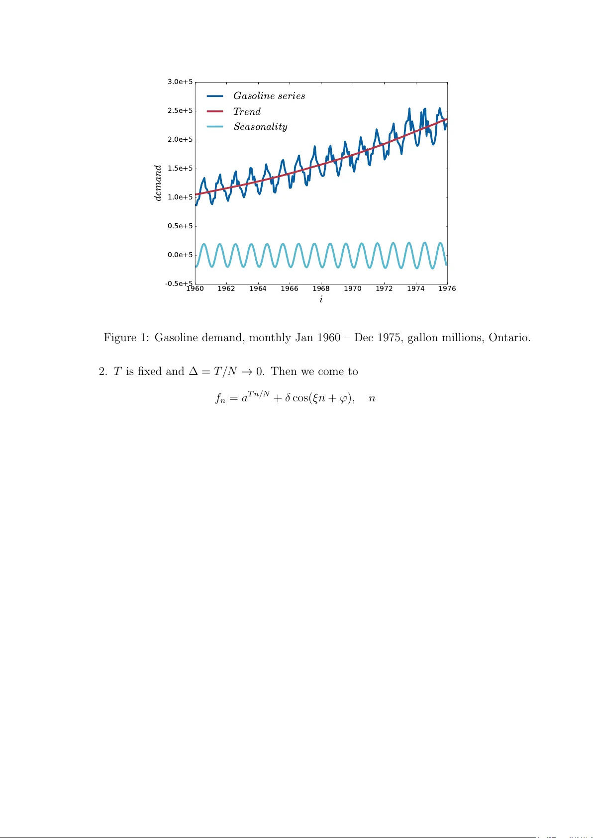
T w o asymptotic approac hes for the exp onen tial signal and harmonic noise in Singular Sp ectrum Analysis Eliza veta Iv ano v a 1 and Vladimir Nekrutkin 2 1 Junior R ese ar cher, Sp e e ch T e chnolo gy Center, 4 Kr asutsky str., St. Petersbur g, 196084, R ussia, E-mail imst563@mail.c om 2 Asso ciate pr ofessor, St. Petersbur g State University, 7/9 Universitetskaya nab., St. Petersbur g, 199034, R ussia, E-mail vnekr@statmo d.ru Abstract The general theoretical approach to the asymptotic extraction of the signal series from the p erturb ed signal with the help of Singular Spectrum Analysis (briefly , SSA) w as already outlined in Nekrutkin 2010, SI I, v. 3, 297–319. In this paper we consider the example of suc h an analysis applied to the increasing exp onen tial signal and the sin usoidal noise. It is prov ed that if the signal rapidly tends to infinit y , then the so-called reconstruction errors of SSA do not uniformly tend to zero as the series length tends to infinity . More precisely , in this case an y finite n umber of last terms of the error series do not tend to an y finite or infinite v alues. On the con trary , for the “discretization” scheme with the b ounded from abov e ex- p onen tial signal, all elemen ts of the error series tend to zero. This effect shows that the discretization mo del can b e an effectiv e to ol in the theoretical SSA considerations with increasing signals. AMS Sub ject Classification 2010 : Primary 65G99, 65F30; secondary 65F15. Keyw ords : Singular Spectrum Analysis, signal extraction, perturbation expansions, asymptotical analysis. 1 In tro duction Let us start with the general construction describ ed in [1]. Consider the real-v alued “signal” series F N = ( x 1 , . . . , x N − 1 ) , 1 < L < N − 1 . T ransfer the series F N in to the Hankel “tra jectory” L × K -matrix H with rows ( x j , . . . , x K + j − 1 ) , where 0 ≤ j < L and L + K = N +1 . It is supp osed that d def = rank H < min( K , L ) . Denote U 0 the eigenspace corresp onding to the zero eigenv alue of the matrix A def = HH T . Then d = dim U ⊥ 0 and dim U 0 = K − d > 0 . Let F N ( δ ) = F N + δ E N b e the p erturb ed signal, where E N = ( e 0 , . . . , e N − 1 ) is a certain “noise” series and δ stands for a formal perturbation parameter. Then w e come to the p erturb ed matrix H ( δ ) = H + δ E with the Hank el matrix E pro duced from the noise series E N . If δ is sufficien tly small, then the linear space U ⊥ 0 ( δ ) spanned by d main left singular v ectors of the matrix H ( δ ) can serv e as an approximation to U ⊥ 0 . The qualit y of this ap- pro ximation can b e measured by the spectral norm   P ⊥ 0 ( δ ) − P ⊥ 0   , where P ⊥ 0 and P ⊥ 0 ( δ ) are orthogonal pro jections on the linear spaces U ⊥ 0 and U ⊥ 0 ( δ ) corresp ondingly . Note that 1   P ⊥ 0 ( δ ) − P ⊥ 0   is nothing but the sine of the largest principal angle b etw een unperturb ed and p erturb ed signal subspaces U ⊥ 0 and U ⊥ 0 ( δ ) . It is w ell-known that a lot of subspace-based metho ds of signal pro cessing are relying on the close pro ximit y of U ⊥ 0 and U ⊥ 0 ( δ ) . Still the main goal of Singular Sp ectrum Analysis (briefly , SSA) is the appro ximation (or “reconstruction”) of the signal F N from the p erturb ed signal F N ( δ ) , see [2] for the detailed description. As it is men tioned in [1, sect. 5], the analysis of the errors of this appro ximation can b e expressed in such a manner. First of all, the “hank elization” (in other terms, “diagonal a veraging”) op erator S is defin ed. If the hank elization op erator S is applied to some L × K matrix Y = { y k,` } L,K k =1 ,` =1 then the resulting L × K matrix S Y has equal v alues denoted b y ( S Y ) j on its an ti-diagonals { ( k , ` ) : such that k + ` − 2 = j }, where j = 0 , . . . , N − 1 , k = 1 , . . . , L and ` = 1 , . . . , K . Besides, ( S Y ) j equals to the av erage of inputs y k,` on this an ti-diagonal. Then, under denotation ∆ δ ( H ) = ( P ⊥ 0 ( δ ) − P ⊥ 0 ) H ( δ ) + δ P ⊥ 0 E , (1.1) the series r 0 , . . . , r N − 1 with r j =  S ∆ δ ( H )  j (1.2) is the series of the reconstruction SSA errors. The peculiarity of the approac h describ ed in [1] can be expressed as follows. The usual metho d of the general p erturbation analysis is to consider the small p erturbation parameter δ and therefore to inv estigate the linear in δ approximation of the problem. F or the subspace- based metho ds this means that N is fixed and δ ↓ 0 , see for example [3] - [6]. Still SSA is usually characterized b y big series length N , and formally this corresp onds to fixed δ and N → ∞ . The mathematical tec hnique that is used in [1] for this goal, go es bac k to [7] and consists of the asymptotic analysis of the corresp onding p erturbation expansions. This paper is devoted to the example of such an analysis for the exp onen tially growing signal and the harmonic noise. This model is not so far from real-life series. F or example, the series “Gasoline demand” (see Fig. 1, data is taken from [8]) can b e approximated by the sum of tw o addends: the increasing trend of the exp onential form and the 12-mon th p erio dicity . Note that b oth trend and p erio dicity in Fig. 1 are pro duced b y SSA with L = N / 2 = 96 . Naturally , the trend is reconstructed b y the first eigen triple of the decomp osition, while the p erio dicity is pro duced with the help of eigentriples 2 and 3. In this pap er w e deal with the follo wing construction. A certain time p erio d [0 , T ] is divided into N in terv als of length ∆ = T / N , and w e consider the signal x n = e θ ∆ n and the noise e n = cos( ξ n + ϕ ) , so that the p erturb ed signal has the form f n = e θ ∆ n + δ cos( ξ n + ϕ ) , n = 0 , . . . , N − 1 , (1.3) where θ > 0 , ξ = 2 π ω with ω ∈ (0 , 1 / 2) , and ϕ ∈ [0 , 2 π ) . As in [1], w e are in teresting in the b ehavior of the reconstruction errors for long signals. F or this goal we consider tw o asymptotic schemes as N → ∞ . 1. ∆ is fixed, further we put ∆ = 1 . Then T = N → ∞ and (1.3) has the form f n = a n + δ cos( ξ n + ϕ ) , n = 0 , . . . , N − 1 (1.4) with a = e θ > 1 . 2 1960 1962 1964 1966 1968 1970 1972 1974 1976 i -0.5e+5 0.0e+5 0.5e+5 1.0e+5 1.5e+5 2.0e+5 2.5e+5 3.0e+5 d e m a n d G a s o l i n e s e r i e s T r e n d S e a s o n a l i t y Figure 1: Gasoline demand, monthly Jan 1960 – Dec 1975, gallon millions, Ontario. 2. T is fixed and ∆ = T / N → 0 . Then we come to f n = a T n/ N + δ cos( ξ n + ϕ ) , n = 0 , . . . N − 1 (1.5) with the same a . F urther w e apply the term “discretization” for this scheme. Note that in b oth cases d = dim U ⊥ 0 = 1 for L, K > 1 . Y et there are considerable differences b et ween (1.4) and (1.5). In particular, the signal of the series (1.4) tends to infinit y as N → ∞ while a T n/ N < a T = const in (1.5). Though the num b er of noise p erio ds tends to infinity in b oth models, the discretization model seems to describ e the real-life situations b etter than (1.4). F or example, the trend of “Gasoline demand” series growths v ery slowly o ver the p erio d of observ ations, while the n umber of p erio ds of the 12-mon th harmonic is relativ ely big. F or b oth mo dels, our in terest lies in the asymptotic b ehavior of   P ⊥ 0 ( δ ) − P ⊥ 0   and of the reconstruction errors. Since the mo del (1.4) corresp onds to the st yle of all examples in [1], sev eral results about this series can be b orrow ed from [1]. In particular, it is already sho wn for (1.4), see [1, sect. 3.2.1], that under the conditions N → ∞ and min( L, K ) → ∞   P ⊥ 0 ( δ ) − P ⊥ 0   = O ( N a − N ) (1.6) and   P ⊥ 0 ( δ ) − P ⊥ 0 − δ V (1) 0   = O ( N 2 a − 2 N ) (1.7) for an y δ ∈ R , where V (1) 0 = P 0 EH T S 0 + S 0 HE T P 0 (1.8) 3 is the linear term of the expansion of P ⊥ 0 ( δ ) − P ⊥ 0 in to p ow er series (see [1, theor. 2.1]), and S 0 stands for the pseudoinv erse of HH T . Besides,   V (1) 0 k = O  N a − N  . Note that in the case L ∼ α N with α ∈ (0 , 1) more careful calculations lead to the precise asymptotic a N √ N   P ⊥ 0 ( δ ) − P ⊥ 0   → | δ | a 2 − 1 a s α ( a 2 − 1) 2( a 2 + 1 − 2 a cos ξ ) (1.9) as w ell as to more precise inequality   P ⊥ 0 ( δ ) − P ⊥ 0 − δ V (1) 0   = O ( N 3 / 2 a − 2 N ) (1.10) instead of (1.7). Since w e omit here pro ofs of b oth (1.9) and (1.10), w e use the inequality (1.7) for the series (1.4) in all further considerations. Section 2 of the pap er is dev oted to the reconstruction errors r j = r j ( N ) for the mo del (1.4). Proposition 2.1 and Corollary 2.1 sho w that r j → 0 as N → ∞ if, roughly sp eaking, j is separated from N . On the con trary , if j is close to N , then r j do es not con verge to zero. Moreov er, the asymptotic b ehavior of r j in this case dep ends on the rationality/irrationalit y of the frequency ω = ξ / 2 π , see prop ositions 2.3 and 2.4. The model (1.5) under the assumption L/ N → α ∈ (0 , 1) is inv estigated in Section 3. It is pro ved in Theorem 3.3 that in this case   P ⊥ 0 ( δ ) − P ⊥ 0   = O ( N − 1 ) as N → ∞ for the sufficien tly small δ . Unlik e the mo del (1.4), the reconstruction errors r j in the discretization scheme tend to zero for all j , see Theorem 3.4. Thus the mo del (1.5) seems to b e more practical than (1.4). In what follo ws, w e alw a ys assume the r e gular b ehavior of the parameter L = L ( N ) as N → ∞ . This means that L ∼ αN with α ∈ (0 , 1) . Still sev eral further inequalities are v alid under less restrictiv e condition min( L, K ) → ∞ . 2 Reconstruction errors for the signal x n = a n Consider the series (1.4) and supp ose that L ∼ α N with α ∈ (0 , 1) as N → ∞ . Our aim is to in vestigate the asymptotic prop erties of the reconstruction errors (1.1), (1.2) for the p erturb ed series (1.4). Since the result of the reconstruction does not c hange if w e reduce H b y H T , assume that L ≤ K . The base of the approac h is the well-kno wn inequality k A k max ≤ k A k , where k A k stands for the usual spectral norm of the matrix A and k A k max = max | a ij | for the matrix A with en tries a ij . Therefore, if k A k is small, then kS A k max is small as well. Th us we rewrite (1.1) in the form ∆ δ ( H ) =  P ⊥ 0 ( δ ) − P ⊥ 0 − δ V (1) 0  H ( δ ) + δ P ⊥ 0 E + δ V (1) 0  H + δ E  . (2.11) It is easy to c hec k that k E k = O ( N ) , k H k = O ( a N ) and k V (1) 0 E k = O ( N 2 a − N ) . Applying (1.7), w e see that k  P ⊥ 0 ( δ ) − P ⊥ 0 − δ V (1) 0  H ( δ ) k = O ( N 2 a − N ) . 4 This means that the reconstruction errors hav e the form r j = r j ( N ) = δ  S ( V (1) 0 H + P ⊥ 0 E )  j + O ( N 2 a − N ) , j = 0 , . . . , N − 1 , (2.12) and all w e need is to inv estigate the asymptotical b ehavior of the series ρ j def =  S ( V (1) 0 H + P ⊥ 0 E )  j =  S ( P 0 EH T S 0 H  j +  S ( P ⊥ 0 E )  j . (2.13) 2.1 The reconstruction errors r j ( N ) in the case N − j → ∞ Let us start with the case when j is not close to N . Prop osition 2.1. Let ρ j = ρ j ( N ) b e defined by (2.13). If L is regular as N → ∞ and N − j → ∞ , then ρ j ( N ) → 0 as N → ∞ . Pr o of. As it w as already men tioned, it is sufficien t to assume that L ≤ K . First of all, for fixed ξ ∈ (0 , π ) , b > 1 , ψ ∈ [0 , 2 π ) and an integer M ≥ 1 denote Φ M ( b, ψ ) = M − 1 X j =0 b j cos( ξ j + ψ ) (2.14) and Υ T ,M ( b, ψ ) = T − 1 X j =0 b j Φ M ( b, ξ j + ψ ) . (2.15) Eviden tly , | Φ M ( b, ψ ) | ≤ ( b M − 1) / ( b − 1) and | Υ T ,M ( b, ψ ) | ≤ ( b M − 1)( b T − 1) ( b − 1) 2 . (2.16) Under the denotation W M = (0 , a, . . . , a M − 1 ) T , P ⊥ 0 = W L W T L k W L k 2 and S 0 = W L W T L k W L k 4 k W K k 2 (2.17) and therefore P ⊥ 0 E + V (1) 0 H = W L W T L k W L k 2 E +  I − W L W T L k W L k 2  EH T W L W T L k W L k 4 k W K k 2 H = W L W T L E k W L k 2 + E W K W T K k W K k 2 − Υ L,K ( a, ϕ ) W L W T K k W L k 2 k W K k 2 = J 1 + J 2 + J 3 . Since  S ( W L W T K )  j = a j and k W M k 2 = ( a 2 M − 1) / ( a 2 − 1) , then     S ( J 3 )  j    = | Υ L,K ( a, ϕ ) | a j ( a 2 − 1) 2 ( a 2 L − 1)( a 2 K − 1) ≤ ( a L − 1)( a K − 1) ( a − 1) 2 a j ( a 2 − 1) 2 ( a 2 L − 1)( a 2 K − 1) = a j ( a + 1) 2 ( a L + 1)( a K + 1) . 5 Let us no w c hec k J 1 and J 2 . In view of the equalities E W K =  Φ K ( a, ϕ ) , Φ K ( a, ξ + ϕ ) , . . . , Φ K ( a, ( L − 1) ξ + ϕ )  T (2.18) and E T W L =  Φ L ( a, ϕ ) , Φ L ( a, ξ + ϕ ) , . . . , Φ L ( a, ( K − 1) ξ + ϕ )  T , w e get that  S ( W L W T L E )  j =                      1 j + 1 j X k =0 a k Φ L ( a, ( j − k ) ξ + ϕ ) for 0 ≤ j < L, 1 L L − 1 X k =0 a k Φ L ( a, ( j − k ) ξ + ϕ ) for L ≤ j < K , 1 N − j N − K X k = j − K +1 a k Φ L ( a, ( j − k ) ξ + ϕ ) for K ≤ j < N . (2.19) In the same manner,  S ( E W K W T K )  j =                      1 j + 1 j X k =0 a j − k Φ K ( a, k ξ + ϕ ) for 0 ≤ j < L, 1 L L − 1 X k =0 a j − k Φ K ( a, k ξ + ϕ ) for L ≤ j < K , 1 N − j N − K X k = j − K +1 a j − k Φ K ( a, k ξ + ϕ ) for K ≤ j < N . Due to (2.16),     S ( W L W T L E )  j    ≤                1 j + 1 a j +1 − 1 a − 1 a L − 1 a − 1 for 0 ≤ j < L, 1 L  a L − 1 a − 1  2 for L ≤ j < K , a j − K +1 N − j a N − j − 1 a − 1 a L − 1 a − 1 for K ≤ j < N . and     S ( E W K W T K )  j    ≤              1 j + 1 a j +1 − 1 a − 1 a K − 1 a − 1 for 0 ≤ j < L, a j L a L − 1 a L 1 a − 1 a K − 1 a − 1 for L ≤ j < K , a j − N + K N − j a N − j − 1 a − 1 a K − 1 a − 1 for K ≤ j < N . Therefore, | ρ j | ≤ 1 j + 1 a + 1 a − 1 a j +1 − 1 a L + 1 + 1 j + 1 a + 1 a − 1 a j +1 − 1 a K + 1 + a j ( a + 1) 2 ( a L + 1)( a K + 1) 6 for 0 ≤ j < L , | ρ j | ≤ 1 L a + 1 a − 1 a L − 1 a L + 1 + 1 L a + 1 a − 1 a L − 1 a L a j a K + 1 + a j ( a + 1) 2 ( a L + 1)( a K + 1) for L ≤ j < K , and | ρ j | ≤ a + 1 a − 1 1 N − j a L − a j − N + L a L + 1 + a + 1 a − 1 1 N − j a K − a j − N + K a K + 1 + a j ( a + 1) 2 ( a L + 1)( a K + 1) if K ≤ j < N . Th us there exist a constant C such that for N big enough | ρ j | ≤ C      a − ( L − j ) / ( j + 1) for 0 ≤ j < L, 1 /L for L ≤ j < K , 1 / ( N − j ) + a − ( N − j ) for K ≤ j < N . (2.20) The pro of is complete. Corollary 2.1. It follows from Prop osition 2.1 that under conditions L/ N → α ∈ (0 , 1) and N − j → ∞ the reconstruction errors r j tend to zero as N → ∞ . Moreo v er, if L ≤ K , then | r j | follo w the same inequalities (2.20) as | ρ j | up to the multiplicator | δ | . 2.2 The reconstruction errors r j ( N ) in the case N − j = O (1) Consider no w the case j = N − 1 − ` with ` = O (1) . Denote G ( a, ξ ) = a 2 − 1 a ( a 2 + 1 − 2 a cos ξ ) . Prop osition 2.2. If ` = O (1) then un der the conditions of Corollary 2.1 r N − 1 − ` = δ G ( a, ξ )  C 1 ( ` ) cos(( N − 1) ξ + ϕ ) + C 2 ( ` ) sin(( N − 1) ξ + ϕ )  + O ( a − L ) , (2.21) where C 1 ( ` ) = 2 1 + `  a cos( `ξ ) − a − ` cos ξ  − ( a 2 + 1 − 2 a cos ξ − 2 sin 2 ξ ) G ( a, ξ ) a − ` and C 2 ( ` ) = 2 1 + `  a sin( `ξ ) + a − ` sin ξ  − 2 sin ξ ( a − cos ξ ) G ( a, ξ ) a − ` . (2.22) Pr o of. F or fixed ξ denote P ( a, n, ψ ) = a cos(( n − 1) ξ + ψ ) − cos( nξ + ψ ) . Straigh tforw ard calculations sho w that Φ M ( b, ψ ) = b M +1 cos(( M − 1) ξ + ψ ) − b M cos( M ξ + ψ ) − b cos( ξ − ψ ) + cos ψ b 2 + 1 − 2 b cos ξ (2.23) and therefore Φ M ( b, ψ ) = b M P ( b, M , ψ ) b 2 + 1 − 2 b cos ξ + O (1) (2.24) for fixed b and M → ∞ . 7 Denote ψ n = ( K − ` − n − 1) ξ + ϕ , then P ( a, L, ψ n ) = P ( a, N − n − `, ϕ ) and ` X n =0 a − n P ( a, N − n − `, ϕ ) = a cos(( N − 1 − ` ) ξ + ϕ ) − cos( N ξ + ϕ ) a − ` . Therefore, taking into accoun t that K ≤ j = N − 1 − ` and applying (2.24) with b = a , M = L and ψ = ψ n , w e get from (2.19)  S ( W L W T L E )  N − 1 − ` k W L k 2 = 1 k W L k 2 1 ` + 1 N − K X k = N − K − ` a k Φ L ( a, ( N − 1 − ` − k ) ξ + ϕ ) = ` X n =0 a N − K − n Φ L ( a, ( K − ` − n − 1) ξ + ϕ ) a 2 − 1 ( ` + 1)( a 2 L + 1) = a 2 − 1 ` + 1 ` X n =0 a L − 1 − n  a L P ( a, L, ψ n ) a 2 + 1 − 2 a cos ξ + O L (1)  1 a 2 L − 1 = a 2 − 1 a ( ` + 1)( a 2 + 1 − 2 a cos ξ ) ` X n =0 a − n P ( a, N − n − `, ϕ ) + O ( a − L ) = = G ( a, ξ ) 1 + `  a cos(( N − 1 − ` ) ξ + ϕ ) − cos( N ξ + ϕ ) a − `  + O ( a − L ) . In the same manner, ( S E W K W T K ) N − 1 − ` k W K k 2 = G ( a, ξ ) 1 + `  a cos(( N − 1 − ` ) ξ + ϕ ) − cos( N ξ + ϕ ) a − `  + O ( a − K ) . No w w e pass to Υ L,K ( a, ϕ ) which is defined in (2.15). It easy to chec k that if b > 1 and T , M → ∞ then Υ T ,M ( b, ψ ) = b S +1 ( b 2 + 1 − 2 b cos ξ ) 2 C ( b, S, ψ ) + O ( b min { T ,M } ) , where S = T + M − 1 and C ( b, S, ψ ) = b 2 cos(( S − 1) ξ + ψ ) − 2 b cos( S ξ + ψ ) + cos(( S + 1) ξ + ψ ) . Therefore, a N − 1 − ` Υ L,K ( a, ϕ ) k W L k 2 k W K k 2 = a 2 N − ` C ( a, N , ϕ ) ( a 2 + 1 − 2 a cos ξ ) 2 ( a 2 − 1) 2 a 2 N +2 (1 − a − 2 L )(1 − a − 2 K ) + O ( a − L ) = = G 2 ( a, ξ ) a ` C ( a, N , ϕ ) + O ( a − L ) . Since a cos(( N − 1 − ` ) ξ + ϕ ) − cos( N ξ + ϕ ) a − ` =  a cos( `ξ ) − a − ` cos ξ  cos(( N − 1) ξ + ϕ ) +  a sin( `ξ ) + a − ` sin ξ  sin(( N − 1) ξ + ϕ ) and C ( a, N , ϕ ) = ( a 2 − 2 a cos ξ + cos(2 ξ )) cos(( N − 1) ξ + ϕ ) + 2 sin ξ ( a − cos ξ ) sin(( N − 1) ξ + ϕ ) , w e get the result in view of (2.12). 8 T o analyze the behavior of the righ t-hand side of (2.21) more precisely , we need some more considerations. First of all, it is w orth to men tion, that C 1 ( ` ) C 2 ( ` ) 6 = 0 for any fixed ` . Th us we can rewrite the result of Prop osition 2.2 in the form r N − 1 − ` = δ F N ( ` ) + O ( a − L ) , (2.25) where F N ( ` ) = D ( ` ) sin  ( N − 1) ξ + ϕ 1 ( ` )  (2.26) with D ( ` ) = a 2 − 1 a ( a 2 + 1 − 2 a cos ξ ) q C 2 1 ( ` ) + C 2 2 ( ` ) and ϕ 1 ( ` ) = arccos C 2 ( ` ) p C 2 1 ( ` ) + C 2 2 ( ` ) ! + ϕ. Remind that ξ = 2 π ω with ω ∈ (0 , 1 / 2) . It is natural that the asymptotic b ehavior of r N − 1 − ` dep ends on the prop erties of the frequency ω . Supp ose that ω = p/q , where p and q are coprime natural num b ers. F or fixed 0 ≤ k < q and ` ≥ 0 consider the sequence N ( k ) m = mq + k + 1 , m ≥ 1 . Since sin  2 π ( N ( k ) m − 1) p/q + ϕ 1 ( ` )  = sin  2 π k p/q + ϕ 1 ( ` )  , then r N ( k ) m − 1 − ` → D ( ` ) sin  2 π k p/q + ϕ 1 ( ` )  as m → ∞ . (2.27) Prop osition 2.3. Let the conditions of Proposition 2.2 be fulfilled. Assume that ` is fixed and that ω is a rational num b er. Denote τ the n umber of limit p oints of the series r N − 1 − ` as N → ∞ . Then τ ≥ 2 . Pr o of. Since D ( ` ) > 0 , it is sufficien t to examine the expressions S ( k ) = sin(2 π k p/q + ϕ 1 ( ` )) with 0 ≤ k < q . If S ( k ) = s = const for all k , then there exist integers m k suc h that 2 π k p/q + ϕ 1 ( ` ) = ( − 1) m k arcsin s + m k π , k = 0 , . . . , q − 1 . Therefore, for 0 ≤ k < q − 1 2 π p/q =  ( − 1) m k +1 − ( − 1) m k  arcsin s +  m k +1 − m k  π = ∆( s, m k , m k +1 ) def =      2 arcsin s + ( m k +1 − m k ) π for ev en m k +1 and o dd m k , − 2 arcsin s + ( m k +1 − m k ) π for odd m k +1 and ev en m k , ( m k +1 − m k ) π , if m k +1 , m k are b oth o dd or even . Since 0 < 2 π p/q < π , then w e immediately come to the inequalit y s 6 = 0 . Supp ose no w that arcsin s > 0 . (The case of arcsin s < 0 can b e treated in the same manner.) Then ∆( s, m k , m k +1 ) ∈ (0 , π ) iff m k +1 − m k = 1 and m k +1 is o dd. Therefore, for an y sequence { m k } q − 1 k =0 with q > 2 there exist a pair ( m k +1 , m k ) with ∆( s, m k , m k +1 ) / ∈ (0 , π ) , and the assertion is prov ed. 9 50 100 150 200 250 300 N 0.002 0.001 0.000 0.001 0.002 0.003 E r r o r s r N − 5 r ( a s ) N − 5 Figure 2: Reconstruction errors r N − 5 and their limit v alues r ( as ) N − 5 for ω = 2 / 9 , L = b 0 . 35 N c , a = 1 . 05 , δ = 0 . 1 , ϕ = 0 and 10 ≤ N ≤ 300 . The con vergence (2.27) and Prop osition 2.3 are illustrated by Fig. 2. T o in v estigate the case of the irrational ω we use the following famous equidistribution theorem going back to P . Bohl [9] and W. Sierpinski [10]. Theorem 2.1. If α ∈ (0 , 1) is irrational, then the sequence z n = { nα } is uniformly dis- tributed on [0 , 1] in the sense that for any 0 ≤ a < b ≤ 1 1 n n X i =1 1 [ a,b ) ( z i ) → b − a, n → ∞ . (2.28) Prop osition 2.4. Let ω ∈ (0 , 1 / 2) b e the irrational num b er and assume ` ≥ 0 to b e fixed. Then for an y ( a, b ) ⊂ [ D ( − ` ) , D ( ` )] and any δ 6 = 0 1 N N + ` X n = ` +1 1 ( a,b ) ( r n − 1 − ` /δ ) → b Z a 1 π p D 2 ( ` ) − u 2 du as N → ∞ . Pr o of. In terms of the weak conv ergence of distributions (see [11] for the whole theory), the con vergence (2.28) means that P n ⇒ U(0 , 1) as n → ∞ , where P n stands for the uniform distribution on the set { z 1 , . . . , z n } , U(0 , 1) is the uniform distribution on [0 , 1] , and “ ⇒ 00 is the sign of the weak conv ergence. No w let us consider the sequence { β n } n ≥ 1 of random v ariables defined on a certain prob- abilit y space (Ω , F , P) and suc h that L ( β n ) = P n for an y n . (Note that here and further L ( β ) stands for the distribution of the random v ariable β .) Then (2.28) can b e rewritten as L ( β n ) ⇒ L ( υ ) as n → ∞ , where υ ∈ U(0 , 1) . A ccording to the Mapping Theorem [11, theor. 2.7], if n → ∞ then L  h ( β n )  ⇒ L  h ( υ )  10 with h ( z ) = D ( ` ) sin  2 π z + ϕ 1 ( ` )  . Standard calculations sho w that the random v ariable η = h ( υ ) has the probability density p η ( z ) = 1 [ − D ( ` ) ,D ( ` )] ( z ) π p D ( ` ) 2 − z 2 , (2.29) where 1 A ( x ) stands for the indicator function of the set A . Since sin(2 π j ω + φ ) = sin  2 π { j ω } + φ  for an y in teger j ≥ 1 , this means that for any a < b 1 N N + ` X n = ` +1 1 ( a,b )  F n ( ` )  → b Z a p η ( u ) du, where F N ( ` ) is defined in (2.26) and N → ∞ . In view of (2.25) the assertion is prov ed. The result of Prop osition 2.4 is illustrated b y Fig. 3. 0.015 0.010 0.005 0.000 0.005 0.010 0.015 r N − 1 0 50 100 150 D e n s i t y Figure 3: Reconstruction errors r N − 1 for ω = √ 2 / 6 , L = b 0 . 35 N c , a = 1 . 05 , δ = 0 . 1 , ϕ = 0 and 10 3 ≤ N ≤ 10 6 . The histogram and the theoretical density (2.29). Remark 2.1. Prop ositions 2.3 and 2.4 sho w that for fixed ` and an y ω ∈ (0 , 1 / 2) the reconstruction error r N − 1 − ` do es not conv erge to an y limit v alue as L/ N → α ∈ (0 , 1) . The case ω = 1 / 2 can b e studied in the same manner and gives the analogous result, while the exp onen tial signal and the constant noise (i.e., the case ω = 0 ) is already c hec ked in [1]. 3 Reconstruction errors for the signal x n = a nT / N No w we deal with the discretization of the exp onential signal, describ ed in the Introduction. More precisely , we consider the constant T > 0 and the triangular array of the series f n = f ( N ) n = a nT / N + δ cos( ξ n + ϕ ) , n = 0 , . . . , N − 1 , N = 1 , 2 , . . . (3.30) 11 under the assumption that N → ∞ and L ∼ αN with α ∈ (0 , 1) . As in the previous section, w e supp ose that a > 1 , ξ ∈ (0 , π ) and ϕ ∈ [0 , 2 π ) . Of course, all form ulas b orro wed from [1] are v alid here. Moreo v er, we can use all general form ulas of Section 2 if w e put a j T /N instead of a j . F or example, now we put W j =  1 , a T / N , . . . , a ( j − 1) T /N  T instead of denotation W j =  1 , a, . . . , a j − 1  T that was used in Section 2. In particular, since rank H = 1 , then the unique p ositive eigen v alue µ of the matrix HH T has the form µ =   W L   2   W K   2 = ( a 2 LT / N − 1)( a 2 K T / N − 1) ( a 2 T / N − 1) 2 . (3.31) T o inv estigate the discretization case we apply t w o general inequalities demonstrated in [1]. Here we put these statements in the form adapted to our problem. Denote B ( δ ) = δ  HE T + EH T  + δ 2 EE T = δ A (1) + δ 2 A (2) (3.32) and let µ b e defined by (3.31). Theorem 3.1. ([1, theor. 2.3]). If δ 0 > 0 and   B ( δ )   /µ < 1 / 4 for an y δ ∈ ( − δ 0 , δ 0 ) , then   P ⊥ 0 ( δ ) − P ⊥ 0   ≤ 4 C k S 0 B ( δ ) P 0 k 1 − 4 k B ( δ ) k /µ with C = e 1 / 6 / √ π . Theorem 3.2. ([1, theor. 2.5]) Put B ( δ ) = | δ | k A (1) k + δ 2 k A (2) k and assume that δ 0 > 0 , B ( δ 0 ) = µ/ 4 and | δ | < δ 0 . Denote A (2) 0 = P 0 A (2) P 0 , then k δ A (2) 0 k < 1 and the matrix I − δ A (2) 0 is in vertible. Besides, under denotation L ( δ ) = L 1 ( δ ) + L T 1 ( δ ) with L 1 ( δ ) = P ⊥ 0 B ( δ ) P 0 µ  I − δ A (2) 0 /µ  − 1 , (3.33) the inequalit y   P ⊥ 0 ( δ ) − P ⊥ 0 − L ( δ )   ≤ 16 C k S 0 B ( δ ) kk S 0 B ( δ ) P 0 k 1 − 4 k B ( δ ) k /µ ≤ 16 C k S 0 B ( δ ) k 2 1 − 4 k B ( δ ) k /µ (3.34) is v alid with the same C as in Theorem 3.1. 3.1 The con v ergence of   P ⊥ 0 ( δ ) − P ⊥ 0   W e start with the norm of B ( δ ) . Lemma 3.1. Assume that L ∼ αN with α ∈ (0 , 1) . Then there exist δ 0 > 0 , N 0 and C suc h that C δ 2 0 < 1 / 4 and k B ( δ ) k /µ ≤ B ( δ ) /µ ≤ C δ 2 for an y δ with | δ | ≤ δ 0 and N > N 0 . 12 Pr o of. First of all, EE T = K 2   1 cos ξ . . . cos(( L − 1) ξ ) . . . . . . . . . . . . cos(( L − 1) ξ ) cos(( L − 2) ξ ) . . . 1   + + sin( K ξ ) 2 sin ξ   cos(( K − 1) ξ + 2 ϕ ) cos( K ξ + 2 ϕ ) . . . cos(( N − 1) ξ + 2 ϕ ) . . . . . . . . . . . . cos(( N − 1) ξ + 2 ϕ ) cos( N ξ + 2 ϕ ) . . . cos(( N + L − 2) ξ + 2 ϕ )   . Since sin ξ > 0 and k A k ≤ √ `k k A k max for an y matrix A : R ` 7→ R k , then k EE T k ≤ LK 2 + | sin( K ξ ) | L 2 sin ξ ∼ α (1 − α ) N 2 / 2 (3.35) as N → ∞ . Using the analogue of (2.18) we see that k HE T + EH T k ≤ 2 k E W K k k W L k ≤ 2 v u u t L − 1 X ` =0 Φ 2 K ( a T / N , ξ ` + ϕ ) a 2 LT / N − 1 a 2 T / N − 1 . (3.36) It can b e c hec ked that | Φ K ( a T / N , ψ ) | ≤ C with a certain constant C = C ( a, T , α, ξ ) that do es not dep end on ψ . F or the further use we denote C 1 = max  C ( a, T , α, ξ ) , C ( a, T , 1 − α, ξ )  . (3.37) Since a 2 LT / N − 1 a 2 T / N − 1 ∼ a 2 αT − 1 2 T ln a N as N → ∞ , then it follows from (3.36) that k B ( δ ) k ≤ B ( δ ) ≤ δ 2 α (1 − α ) 2 N 2 + o ( N 2 ) . In view of the asymptotic µ = ( a 2 αT − 1)( a 2(1 − α ) T − 1) 4 T 2 ln 2 a N 2 + o ( N 2 ) , (3.38) the pro of is complete. Theorem 3.3. Under the conditions of Lemma 3.1,   P ⊥ 0 ( δ ) − P ⊥ 0   = O ( N − 1 ) as N → ∞ . Pr o of. Due to Theorem 3.1 and Lemma 3.1, all w e need is to pro of that k S 0 B ( δ ) k = O (1 / N ) . (3.39) By (2.17), S 0 B ( δ ) = δ D 1 k W L k 2 k W K k 2 + δ D 2 k W L k 4 k W K k 2 + δ 2 D 3 k W L k 4 k W K k 2 (3.40) 13 with D 1 = W L W T K E T , D 2 = W L W T L E W K W T L , and D 3 = W L W T L EE T . (3.41) Consider summands in the righthand side of (3.40) separately . First of all , D 3 D T 3 = W L W T L EE T EE T W L W T L = W L W T L L − 1 X i =0 L − 1 X j =0 a j T /N Ψ K ( ϕ, i, j ) ! 2 , where Ψ M ( ψ , k , ` ) = M − 1 X j =0 cos( ξ ( j + k ) + ψ ) cos( ξ ( j + ` ) + ψ ) . (3.42) Since L − 1 X j =0 a j T /N Ψ K ( ϕ, i, j ) = K 2 Φ L ( a T / N , − iξ ) + sin( K ξ ) 2 sin ξ Φ L ( a T / N , iξ + ( K − 1) ξ + 2 ϕ ) , (3.43) w e get k D 3 k 2 ≤ a 2 T L/ N − 1 a 2 T / N − 1  C 2 1 K 2 L 4 + O ( LK )  = a 2 αT − 1 2 T ln a C 2 1 (1 − α ) 2 α 4 N 4 + o ( N 4 ) with C 1 defined in (3.37). Thus k D 3 k  k W L k 4 k W K k 2  − 1 = O (1 / N ) . In the same manner, D 2 = W L W T L L − 1 X i =0 a iT / N Φ K ( a T / N , iξ + ϕ ) and k D 2 k ≤ C 1 r a 2 αT − 1 2 a αT − 1 ( T ln a ) 3 / 2 N 3 / 2 + o ( N 3 / 2 ) . Therefore, k D 2 k  k W L k 4 k W K k 2  − 1 = O (1 / N ) . Lastly , D 1 D T 1 = W L W T K E T E W K W T L = W L W T L L − 1 X i =0 Φ 2 K ( a T / N , iξ + ϕ ) . Since P L − 1 i =0 Φ 2 K ( a T / N , iξ + ϕ ) ≤ LC 2 1 , then k D 1 k 2 ≤ a 2 T 0 L/ N − 1 a 2 T 0 / N − 1 C 2 1 L = α a 2 αT − 1 2 T ln a C 2 1 N 2 + o ( N 2 ) , k D 1 k  k W L k 2 k W K k 2  − 1 = O (1 / N ) and the pro of is complete. 14 3.2 Reconstruction errors T o in vestigate the reconstruction errors w e use the same idea as in Section 2 but deal with the inequalit y (3.34) instead of (1.7) and use the expression ∆ δ ( H ) =  P ⊥ 0 ( δ ) − P ⊥ 0 − L ( δ )  H ( δ ) + δ P ⊥ 0 E + L ( δ ) H + δ L ( δ ) E . (3.44) instead of (2.11). F or this goal, we need the following supplementary assertions. Lemma 3.2. Denote Z = δ A (2) 0 /µ = δ P 0 EE T P 0 /µ . Then there exists a constan t C 2 suc h that k Z k max ≤ | δ | C 2 / N (3.45) with k Z k max = max m,`   Z [ m, ` ]   . Pr o of. First of all, A (2) 0 [ m, ` ] = EE T [ m, ` ] − EE T W L W T L [ m, ` ] k W L k 2 − W L W T L EE T [ m, ` ] k W L k 2 + W L W T L EE T W L W T L [ m, ` ] k W L k 4 . Note that EE T [ m, ` ] = Ψ K ( ϕ, m, ` ) , where Ψ M ( ψ , k , ` ) is defined in (3.42). Analogously , EE T W L W T L [ m, ` ] = a `T / N L − 1 X j =0 a j T /N Ψ K ( ϕ, m, j ) , W L W T L EE T [ m, ` ] = a mT / N L − 1 X j =0 a j T /N Ψ K ( ϕ, j, ` ) , and W L W T L EE T W L W T L [ m, ` ] = a ( ` + m ) T / N L − 1 X k,j =0 a ( j + k ) T / N Ψ K ( ϕ, k , j ) . In view of (3.43), EE T W L W T L [ m, ` ] k W L k 2 + W L W T L EE T [ m, ` ] k W L k 2 + W L W T L EE T W L W T L [ m, ` ] k W L k 4 = O (1) . Since Ψ K ( ϕ, m, ` ) = K cos( ξ ( m − ` )) / 2 + O (1) as K → ∞ , then A (2) 0 [ m, ` ] = cos(( m − ` ) ξ ) 2 K + o (1) uniformly in 0 ≤ m, ` ≤ L − 1 . Therefore, see (3.38), Z [ m, ` ] = δ cos(( m − ` ) ξ ) 2(1 − α ) T 2 ln 2 a ( a 2 αT 0 − 1)( a 2(1 − α ) T 0 − 1) 1 N + o (1 / N ) and the pro of is complete. Remark 3.1. As the consequence of the inequality (3.45) w e get that for any n ≥ 1 k Z n k max ≤ | δ | n C n 2 / N . Since k Z n k max ≤ L k Z n − 1 k max k Z k max , this fact can b e pro ved with the help of a simple induction. Therefore, if | δ | C 2 < 1 , then    X n ≥ 1 Z n    max ≤ X n ≥ 1 k Z n k max ≤ | δ | C 2 1 − | δ | C 2 1 N . (3.46) 15 Lemma 3.3. If the series f n = f ( N ) n is defined b y (3.30), N → ∞ and L ∼ α N with α ∈ (0 , 1) , then 1) k B ( δ ) H k max = O ( N ) ; 2) k S 0 B ( δ ) k max = O (1 / N 2 ) ; 3) k B ( δ ) S 0 E k max = O (1 / N 2 ) and 4) k P ⊥ 0 E k max = O (1 / N ) . Pr o of. 1) The matrix B ( δ ) H can b e rewritten as follows: B ( δ ) H = δ k W L k 2 J 1 + δ J 2 + δ 2 J 3 with J 1 = E W K W T K , J 2 = W L W T K E T W L W T K and J 3 = EE T W L W T K . Applying the equalities (2.15) and (3.42), (3.43) we get that k J 1 k max = max k 1 and ξ ∈ (0 , π ) , ϕ ∈ [0 , 2 π ) . If N → ∞ and L = αN + o ( N ) with 0 < α < 1 , then there exists δ ∗ > 0 such that r j = O (1 / N ) uniformly in 0 ≤ j < N for an y δ with | δ | < δ ∗ . Pr o of. First of all, see Lemma 3.1, the inequality (3.34) holds for an y δ suc h that | δ | < δ 0 . Then, due to (3.44), P ⊥ 0 ( δ ) H ( δ ) − P ⊥ 0 H =  P ⊥ 0 ( δ ) − P ⊥ 0 − L ( δ )  H ( δ ) + L ( δ ) H + δ L ( δ ) E + δ P ⊥ 0 E . (3.47) It follo ws from (3.34) and (3.39) that k  P ⊥ 0 ( δ ) − P ⊥ 0 − L ( δ )  k = O (1 / N 2 ) for | δ | < δ 0 , and therefore    P ⊥ 0 ( δ ) − P ⊥ 0 − L ( δ )  H ( δ )   ≤    P ⊥ 0 ( δ ) − P ⊥ 0 − L ( δ )    k H ( δ ) k = O (1 / N ) . Th us we must chec k the tree last terms in the righthand side of (3.47). Note that k P ⊥ 0 E k max = O (1 / N ) , see Lemma 3.3. Let us consider op erators L ( δ ) H and L ( δ ) E . As in Lemma 3.2, put Z = δ A (2) 0 /µ . Since P 0 H = 0 , then ZH = 0 and L 1 ( δ ) H = S 0 B ( δ ) P 0  I − Z  − 1 H = S 0 B ( δ ) P 0 X m ≥ 0 Z m H = 0 . Therefore, L ( δ ) H = L T 1 ( δ ) H =  I − Z  − 1 P 0 B ( δ ) H µ = 1 µ I + X m ≥ 1 Z m ! P 0 B ( δ ) H = 1 µ P 0 B ( δ ) H + 1 µ X m ≥ 1 Z m P 0 B ( δ ) H = 1 µ P 0 B ( δ ) H + 1 µ X m ≥ 1 Z m ! B ( δ ) H . Since P ⊥ 0 = W L W T L / k W L k 2 and k W L W T L k max ≤ a 2 T , then k P ⊥ 0 k max = O (1 / N ) and, in view of Lemma 3.3,   P 0 B ( δ ) H /µ   max =    I − P ⊥ 0  B ( δ ) H /µ   max ≤ k B ( δ ) H k max µ +   P ⊥ 0 B ( δ ) H   max µ ≤ k B ( δ ) H k max µ + L   P ⊥ 0   max k B ( δ ) H k max µ = O (1 / N ) . Besides, if additionally | δ | C 2 < 1 , then, due to (3.38) and (3.46),    1 µ  X m ≥ 1 Z m  B ( δ ) H    max ≤ L µ    X m ≥ 1 Z m    max    B ( δ ) H    max ≤ L µ | δ | C 2 1 − | δ | C 2 1 N    B ( δ ) H    max = O (1 / N ) . As the result, k L ( δ ) H k max = O (1 / N ) . By definition, L ( δ ) E = L 1 ( δ ) E + L T 1 ( δ ) E with L 1 ( δ ) E = S 0 B ( δ ) P 0  I − Z ) − 1 E and L T 1 ( δ ) E =  I − Z ) − 1 P 0 B ( δ ) S 0 E . The equalit y k L T 1 ( δ ) E k max = O (1 / N 2 ) can b e demonstrated in the same manner as k L T 1 ( δ ) H k max = O (1 / N ) , with the help of the equality k B ( δ ) S 0 E k max = O (1 / N 2 ) (see Lemma 3.3). 17 No w note that L 1 ( δ ) E = S 0 B ( δ ) P 0 E + S 0 B ( δ ) P 0 X m ≥ 1 Z m ! E = S 0 B ( δ ) P 0 E + S 0 B ( δ ) X m ≥ 1 Z m ! E . T aking into account (3.46) and equalities k E k max = O (1) , k S 0 B ( δ ) k max = O (1 / N 2 ) w e get     S 0 B ( δ )  X m ≥ 1 Z m  E     max ≤ L 2 k S 0 B ( δ ) k max    X m ≥ 1 Z m    max k E k max = O (1 / N ) . Lastly , k S 0 B ( δ ) P 0 E k max ≤ k S 0 B ( δ ) E k max + k S 0 B ( δ ) P ⊥ 0 E k max ≤ L k S 0 B ( δ ) k max k E k max + L 2 k S 0 B ( δ ) k max k P ⊥ 0 k max k E k max = O (1 / N ) . Therefore, k L ( δ ) E k max = O (1 / N ) . Finally , the uniform norm k · k max of each addend in the sum (3.44) has the order O (1 / N ) . Since kS C k max ≤ k C k max for any matrix C , the pro of is complete. References [1] Nekr utkin, V. (2010). Perturb ation exp ansions of signal subsp ac es for long signals. Statistics and Its Interface. 3 297–319. [2] Gol y andina, N., Nekr utkin, V. and Zhiglja vsky, A. (2001). A nalysis of Time Series Structur e. SSA and R elate d T e chniques. Champan & Hall/CRC, Bo ca Raton- London-New Y ork-W ashington D.C. [3] Badea u, R., Ga ¨ el Richard, G., and D a vid, B. (2008). Performanc e of ESPRIT for Estimating Mixtur es of Complex Exp onentials Mo dulate d by Polynomials. IEEE T ransactions on Signal Pro cessing. 56 , 1, 492-–504. [4] Gol y andina, N., Vlassiev a, V. (2009). First-or der SSA-err ors for long time se- ries: mo del examples of simple noisy signals. In: Proceedings of the 6th St.Petersburg W orkshop on Simulation V ol.1, June 28-July 4, 2009, St. Petersburg, VVM com.Ltd., 314-319. [5] Hassani, H., Xu, Zh. and Zhiglja vsky, A. (2011). Singular sp e ctrum analysis b ase d on the p erturb ation the ory. Nonlinear Analysis: Real W orld Applications, 12 , 5, 2752– 2766. [6] Vr onska y a-R ob, M., Schmidt, K. (2017). On p erturb ation stability of SSA and MSSA for e c asts and the supp ortiveness of time series. Statistics and Its In terface, 10 , 1, 33-–46. [7] Ka to, T. (1966). Perturb ation the ory for line ar op er ators . Springer-V erlag, Berlin- Heidelb erg-New Y ork. [8] Abraham, B., Ledol ter, J. (1983). Statistic al Metho ds for F or e c asting . Wiley Series in Probabilit y and Statistics, Wiley . 18 [9] Bohl, P. (1909). ¨ Ub er ein in der The orie der s¨ akutar en St¨ orungen vorkommendes Pr oblem . J. reine angew. Math. 135 189-283. [10] Sierpinski, W. (1910). Sur la valeur asymptotique d’une c ertaine somme , Bull In tl. A cad. Polonmaise des Sci. et des Lettres (Cracovie) series A, 9-11. [11] Billingsley, P. (1999). Conver genc e of pr ob ability me asur es , 2-nd edition, Wiley series in probabilit y and statistics, Wiley , New Y ork-Chic hester-W einheim-Brisbane- Singap ore-T oronto. 19