Performance Bounds for Parameter Estimation under Misspecified Models: Fundamental findings and applications
Inferring information from a set of acquired data is the main objective of any signal processing (SP) method. In particular, the common problem of estimating the value of a vector of parameters from a set of noisy measurements is at the core of a ple…
Authors: ** S. Fortunati, F. Gini, M. S. Greco (University of Pisa
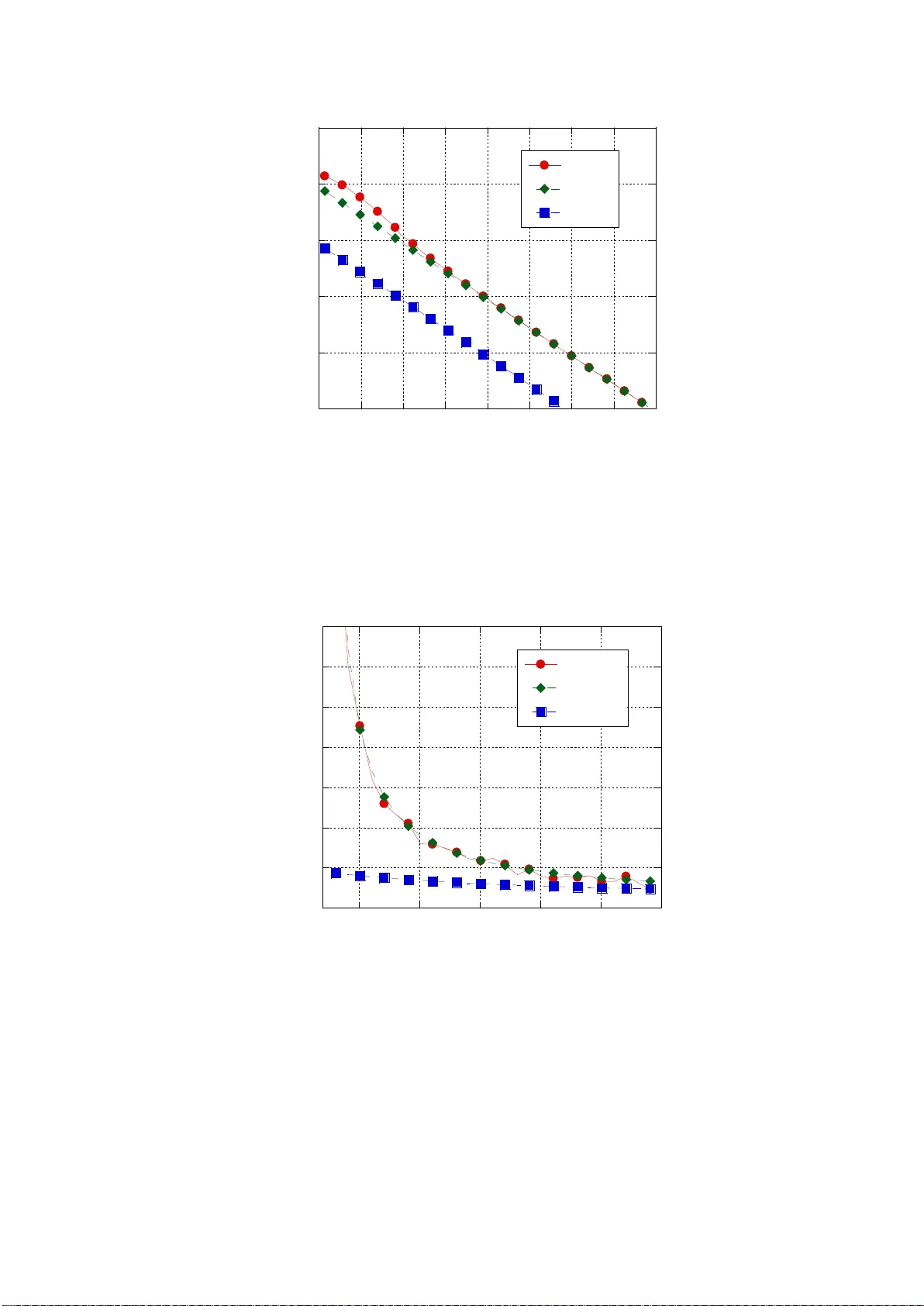
1 Performance Bound s for Param eter Estimation under Misspecif ied Models: Fund amental findings and applications S. Fortunati 1 , F. Gini 1 , M. S. Greco 1 , and C. D. Richmond 2 1 Dipartimento di Ingeg neria dell’I nformazione, Universit y of Pisa , Italy 2 Arizona State University, School of Electrical, Computer and Energy En gineering, Tempe, USA. A BSTRACT Inferring information f rom a set of acqu ired data is the main objective of any signal pro c- essing ( SP) method. In particular, the common problem of est imating the value of a vector of parameters from a set of noisy measure ments is at the core of a plethora of scientific and technological advances in the last decades; for example, wireless comm unications, radar and sonar, biomedicine , image process ing, and seismolog y, just to name a few. Developing an estim ation algorithm o ften begins by assuming a st atistical m odel for the measured data, i.e. a probabil ity density function (pdf), which if correct, fully char acterize s the behaviour of t he collected data/measurements. Experience with real data, howev er, often exposes the limitations of any assumed data model since modelling errors at som e level are always present. Consequen tly, the true data model and the model assumed to derive the est i- mation algorithm could differ. When this happens, the model i s said to be mismatched or mi s- specified . Therefore, understand ing the possib le performance loss o r regret t hat an estimation algorithm could experience under model misspecification is of cruc ial importance for any SP practitioner. Further, und erstanding the limits on the perfor mance of any estimator subject to model m isspecification is of practical intere st. Motivated by t h e widespread and practical need to assess the performance of a “mi s- matched” estimator , th e goal of this paper is to help to bring attention to the main theoretical 2 fi ndings on estimation theory, and in particular on lower bounds under model misspecific a- tion, that have been published in the statistical and econometrical literature in the last fifty years. Secondly, some applications are discussed to illustrate the broad range of areas and problems to which this framework extends , and consequently the numerous opportunities available for SP re searche rs . 1. I NTRODUCTION The mathem atical basis for a formal theory of statistica l inference w as presented by Fisher, who introduced the Maximum Likelihood (ML) method along with its main properties [Fis25]. S ince then, ML estimation has been widely used i n a variety of applications. One of the main reasons for its popularity is its asym ptotic efficiency, i .e. its ability to achieve a minim um value of the erro r variance as the number of available observ ations goes to infini ty or as the noise power decreases to zero. T he concept of efficiency is strictly related to the ex- istence of some lower bounds on the performance of any estimator designed for a specific i n- ference task. Such perform ance bounds, one of which is the celebrated Cram ér-Rao Bound (CRB) [Cra46] [Rao45], are of fundamental importance in practical applicati ons since t hey provide a benchmark of com parison for the performance of any estimator. Specifi cally, given a particular estimation problem, if the perform ance of a certain algorithm ac hieves a relevant performance bound, then no other algorithm can do better. Moreover, evaluat ing a perfo r- mance bound is often a prerequisi te for any feasibility study. I n particular, the availability of a lower bound for the estimation problem at hand makes the SP practitioner aware of the pract i- cal impossibility to achieve better estimation accurac y than t he one i ndicate d by the bound itself. Another fundamental feature of a perform ance bound i s its ability to cap ture and reveal the complex dependence s am ong st the various paramet ers of interest, t hus offering the oppo r- tunity to understand more deeply the estimation problem at hand and ultimately to i dentify an appropriate desig n choice of param eters and criterion for an estim ator [Kay98]. 3 Before describing specific performance bounds, it is worth mention ing that estimation th e- ory explores two different fram eworks: one i s determin istic and one i s Bayesian . In the class i- cal deterministic approach, t he parameters to be estim ated are modelled as determinis tic but unknown variables. This im plies that no a-priori information is available that would suggest that one outcome is more or less likely than another. In the Bay esian framework instead, the parameters of interest are assumed to be random variabl es and the goal is to estimate their particular realizations. Unlik e t he cl assical deterministi c approach, the Bayesian approach ex- ploits th is random characterization o f the unknown parameters by incorporating a-priori in- formation about the unknown parameters in the derivation of an estim ation algorithm. In pa r- ticular, the joint pd f of the unknown param eters is assum ed known, and therefore can be tak en into account in the estimation process through Bayes’ theorem [Kay98]. 1.1 B ASICS ABOUT PERFORMANCE BOUNDS When talking about lower bounds, the first distinction that needs to be made is between local (or small-error) bounds and global (or large-error) bounds. A bound can be considered a local error bound if its calculation relies exclus ively on the b ehaviour of the pdf of the data at a single point value of t he parameter ( or perhaps a very small “local” neighbourhood around this point). I f the calculation of a bound requires knowledge of the pdf behaviour at multiple (more than one) distinct and well separated (non- local) points, then the bound can be characterized as a global error bound. Local error bounds at best determine the limits of the asymptotics of optim al algorithms like ML, whereas characterization of non -asym ptotic pe r- formance m ust somehow take into account the possible influence of parameter values other than the true v alue. A bound is said to be “tight” if it reasonably predicts the perform ance of the ML estim ator. In part icular, if a bound is only as ym ptotically tight, then it is reliable only in t he presence of high Signal- to - Noise Ratio (SNR) or sufficiently large number of measurements. On the other hand, if a b ound is globally t ight, then it is a reliable bound for the error covariance of an ML 4 estimator irrespective of t he S NR level or of the amount of available data. The determ inistic bound t hat can be regarded as the most general representative of the class of global bounds is the Barankin Bound (BB) [ Bar49]. However, due to its generality, the calculation of the BB is not straig htforward and it usually does not admit a closed form representation. T he most po p- ular local bound is the above-m entioned CRB. Unlike the BB, the CRB is easy to evaluate for many practical problem s, but it is reliable only asymptotical ly . In the non-asym ptotic region, which is characterized by a low SNR and/or by a l ow number of m easure ments, the CRB can be “too optim istic” with respec t t o the effective error covariance achievable by an estimator [Van13]. The second subdiv ision of the perform ance bounds is a di rect consequence of the di cho t- omy between the determ inistic and the Bayesian estimation frameworks. In particular, we can identify the class o f deterministic lower bounds and the class of Bayesian lower bounds [Van07]. Without any cl aim of completeness, the class of the deterministic lower bounds in- cludes: the (global) BB [Bar49], and two local bounds, the Bhattacha ryya Bound [Bha46] and the CRB [Cra46] [Rao45]. We stress that the most comm on forms of these bounds, including the CRB , apply only to unbiased estimators. Versio ns of these bounds exist, how ever, that can be applied to bia sed estimators whose bias function can be determined. Concerning the Bayesian bounds, t hey can be di vided into two classes [Ren08] : the Ziv- Za kaï family and the Weiss-Weinste in family, to which the Bayesian version of the CRB belongs . The first family is derived by relating mean squa red error to the probability of error in a binary hypothesis testing problem, while the derivation of the l atter is b ased on the covariance i ne quality. For further details on B ayesian Bounds, we refer the reader to the comprehensiv e book [Van07]. 1.2 A N ESTIMATION THEORY UNDER MODEL MISSPECIFICATION : MOTIVATIONS Regardless of the differences previously discussed, both the classical deterministic estim a- tion theory and the Bayesian framework are based on the implicit assum ption that t he a s- sumed dat a m odel, i.e. the pdf, an d the true data model are t he sam e, i.e. the m odel is co r- 5 rectly spec ified . However, much evidence from engineering pr actice shows that this assum p- tion is often violated, i.e. the assum ed model is different from t he true one. There are two main reasons for model misspecificatio n . The first is the imperfect knowledge of the true data model, which leads t o an incorrect specifica tion of the data pdf. On the other hand, t here could be cases where perfect knowledg e of the true data model i s available but, due to an i n- trinsic computa tional complex ity or to a costl y hardware implementation, it is not possible nor convenient to pursue the opt i mal “matched” estim ator. I n these cases, one may prefer to derive an estimator by as sum ing a si mpler but misspecified data model, e.g. t he Gaussian model. Of course, this suboptimal procedure may lead to some degradation in the overall sy s- tem performance, but ensur es, on the other hand, a sim ple analytical deriv ation and real-time hardware implem entation of the inference algorithm. I t is clear that, i n such a misspecified estimation fram ework, the possibility t o assess t he impact of the model misspecificat ion o n the esti m ation performance is of fundam ental importance to guarantee the reliability of the (mism atched) estimator. Misspecified bounds are then the perfect candidates to fulfil this task: they generalize the classical framework by allowing the assumed a nd true models to di f- fer, yet they es tablish performance limits on the estimation error covariance in a way that i n- dicates h ow t he diff erence between the tr ue and assum ed m odels affects the estimation pe r- formance. Having es tablish ed the main m otivations, we can now briefly review the literature on t he estimation framework under model misspecification, with a focus on the two classica l building block s, i.e. the ML estim ator and the CRB. 1.3 S OME HISTORICAL BACKGROUND The first fundamental result on the behaviour of the ML estimator under misspecificat ion appeared in the statistical literature in t he year 1967 and was provided by Huber [Hub67]. In that paper the cons istency and the normality of the ML es tim ator were proved under very mild regularity conditions. Five years later, Akaike [Aka72 ] highlighted the link between Huber’s findings and the Kullback-Leibler divergence (KLD) [Cov06]. He noted that t he convergence point of the ML estimator under model misspecif icatio n could be i nterpreted as 6 the point that minimizes the KLD between the true and the assumed models. In the early 80’s, these ideas were further developed by White [Whi8 2 ], where the term “Quasi -Maximum Likelihood” (QML) estimator was intro duced. Som e y ears later, the second fundam ental building blo ck of an estim ation theory under model m isspecification was e stablished by Vuong in [Vuo86 ]. Vuong was the first one to derive a generalization of the Cramér-Rao lower bound under misspecified models. Analysis of the Bayesian misspecified estimation problem has been inv estigated in [Ber66 ] and [Bun98 ]. Quite surpr isingly and despite the wide v ariety of potential applications, the SP comm u- nity has remained largely unaware of these fundamental r esu lts . Only r ecently, this topic ha s been red iscovered and its application s to well- kn own SP problems investigated ([Xu04], [Noa07], [ Ric13 ], [Gre14], [Gus14], [Ric15], [Kan15 ], [Par15], [ Ren15], [Fri15], [For16a], [For16b], [For16c], [Ric16], [ Men18] ). Of course, every SP practitioner was well aware of the misspec ification problem, but some approach es comm only used within the SP community to address it differed from some of th ose proposed in the sta tistical literature. I n particular, the effect of the misspecific ation has been modelled by adding i nto the true data model some ran- dom quanti ties, also called nuisance parameters , and by trans form ing the estimation problem at hand in to a higher dimensional hybrid estim ation problem. The performance degradation due to the augm ented level of uncertainty generated by the nuisance param eters could be a s- sessed by evaluating the t rue CRB when possible, t he hybrid CRB (see, e.g. [Roc87] , [Gin00], [Par08], [Noa09]), or the m odified CRB ([And92], [Gin98], [Kba17]). T his ap- proach, although reasonab le, is application-depende nt and not general at all. Other approach es include sensitiv ity analyses [Fr i90] , [Van1 3]. Finally, it could also be of i nterest to point out here the relationship between misspecified estimation theo ry and robust (see [Zou12 ] for an excellent tutori al on robust statistics ) . As one would expect, these t wo framework s share t he same motivations, i .e. an imperfect knowledge of the true data model. The aim of r obust estimation theory is to develop estim ation algo- rithms ca pable of achieving good performance over a l arge set of allowabl e input data m o d- 7 els, even if suboptim al under any nominal (or true) model. Even though the development of robust estimators ar e surely of great i mportan ce in ma ny SP applications, for som e of these the mathematical derivation and consequent implem entati on may be t oo involv ed or too time and hardware intensive. In these cases, as discussed before, one may prefer to apply the cla s- sical, non - robust, estim ation theory by assum ing a simplified , h ence misspeci fied, statistical model for the dat a. The first aim of this article is to summ arize the most relevant existing works in the statist i- cal literature using a formalism that is more familiar to the SP community . Secondly, we aim to show the potential appl ication of misspeci fied estim ation theory, in both the deterministic and Bayesian con texts, to various cla ssical SP problems. 2. D ESCRIPTION OF A MISSPECIFIED MODEL PROBLEM Let 1 , , M x x be a set of N -dimensional (generally complex) random vector s, r epre senting the outcome of a measurem ent process. Let N m x be a single observation vector with probability density f unctio n (p df ) () Xm p x belonging t o a possibly parametric f amily, or model , that charac terizes the observed ran dom experim ent. As discussed in Sect. 1 , in a l- most all practical applications the true pdf () Xm p x ei ther is not perfectly known, o r it does not adm it a simple derivation or easy implementation of the estimation alg orithm . Th us, in- stead of () Xm p x , in t he mismatched estim ation framework we adopt a different parametric pdf, say ( | ) Xm f x θ with d θ , to characterize the statistical behaviour of the data ve c- tor m x . Potential estim ation algorithms may be deri ved from the misspecified parametric pdf ( | ) Xm f x θ belonging to a paramet ric model and not from the true pdf () Xm p x . Mor e- over, we assume t hat ( | ) Xm f x θ could differ from () Xm p x for every θ . Since this a s- sumption represents the di v ision bet ween the classical matched and the misspecif ied parame t- ric estimation theories, some additional comm ents are warranted. The matched estimation theory requires the existence of at l east a param eter ve ctor θ for which t he pdf assum e d 8 by the SP practitioner is equal to the t rue one. Mathe matically, we can say that the classical matched theory holds true i f, for some θ , ( ) ( | ) X m X m pf xx θ , or equivalently if () Xm p x . For exa mple, suppose that the collected data, i.e. the outcomes of a random e x- periment, are dis tributed according to a univariate Gaussian distribution with m ean value and variance 2 , namely, 2 ( ) ( , ) m X m x p x , 1 , , m M . Moreover, suppose that the assum ed parametric model for data in ference is the Gaus sian parametri c model, i.e. 12 { | ( | ) ( , ) } X X m f f x θθ , where i s the set of positi ve rea l number s . This situation clearly represents a matched case, since there exists 2 ( , ) θ such that ( ) ( | ) X m X m p x f x θ = 2 ( , ) . Suppose now that the collected data are actually di s- tributed acco rding to a univariate Lap lace distributio n with l ocation parameter and scale parameter , i.e. ( ) ( , ) m X m x p x . Due to perhaps misleading and incomplete info r- mation on the experim ent at hand, or due to the need to derive a simple algorithm, we decide to adopt a parametric Gaussian model to characteriz e the collected data. Unlike the prev i- ous case, this is obviou sly a mismatched case, since there does not exist any 12 ( , ) θ for which the assum ed Gaussian m odel is equal to the true Laplace model. Many pr actical examples of model misspecification can be f ound in the everyday eng i- neering practices. J ust to nam e a few, recent papers have investigated t he applic ation of this misspecifed model framework to the Direction-of-Arrival (DoA) estimation problem in se n- sor arrays ([Ric13],[Ri c15],[Kan15]) and MIMO radars [Ren15], to the covariance matrix e s- timation problem in non-Gaussian distur bance ([Gre14], [For16a], [For16c]), to radar- communication systems coexistence [Ric16], to wave form parameter estim ation in the pre s- ence of uncertainty in the propagation model [Par15] , and to the Time-of-Arrival (ToA) est i- mation problem fo r ultra wi deband (UWB) signals in t he presence of interf erence [Gus14]. Since the first part of the paper deals with the determ inistic misspecified es timation theory , the par ameter vector θ is assum ed t o be an unknown and determ inistic real vecto r. T he ex- 9 tension to the Bayesian case is discussed in Sect. 5. Suppose that for inference purposes we collect M i ndependent, identical ly distributed (i.i.d.) measurem ent vectors 1 {} M mm xx , where () m X m p x x . Due to the independ ence, the true joint pdf of the dataset x can be expressed as the product of t he marginal pdf as 1 ( ) ( ) M X X m m pp xx . The assumed j oint pdf of the dataset is instead 1 ( | ) ( | ) M X X m m ff x θ x θ . This misspecifi ed model fram ework raises two important ques tions: I s it still possible to derive lower bounds on the error covariance of any mi s- matched estim ator of the param eter vector θ ? How will the classical statistical properties of an estimator , e.g. unbiasedness, co n- sistency and effi ciency, chang e in this misspecified model fram ework? What is the meaningfu lness of parameter estimates under extrem e cases of mi s- match? The remainder o f th is paper addr ess es these fun damental issues. 3. T HE M ISSPECIFIED C RAMÉR -R AO B OUND This section i ntroduce s a version of the CRB accounting for poss ible mo del misspecific a- tion, i.e. the misspecified Cramér- Rao bound (MCRB), which can be cons idered a generaliz a- tion of the usual CRB, which is obtained when the model is corr ectly specified. We start by providing the require d regularity conditions and the notion of unbiasedness for m ismatched estimators. 3.1 R EGULAR MODELS As with the class ical CRB, in order to guarantee the e xistence of the MCRB, som e regula r- ity conditions on the assum ed pdf need to be imposed. Specifically , the assumed parametric model has to be regular with respect to (w.r.t.) , i.e. the family to which the true pdf belongs. The complete list of assum ptions that has to sa tisfy to be regular w.r.t. are 10 given in [Vuo86] and brief ly recalled in [ For16a ]. Most of them are rather technical and f a- cilitate order reversal of integral and derivative operators. Neverthe less, there are two a s- sumptions that need to be discussed here due t o thei r importance in the develop ment of the theory. The firs t condition that has to be sat isfied is: A1. There exist s a unique interior po int 0 θ of such that 0| ar g m in ln | ar g m in p X m X X E f D p f θ θθ θ x θ , (1) where p E indicates the expectation operator of a vector - or scalar-v alued fun c- tion w.r.t. the pdf () Xm p x and | l n ( ( ) ( | )) ( ) X X X m X m X m m D p f p f p d θ xx θ x x is the KLD [Cov06] betwee n the true and the assumed pdfs. As indicated by eq. (1), 0 θ can be interpreted as the point that minimiz es the KLD between () Xm p x and ( | ) Xm f x θ and it is called the p seudo-true parame ter vector ([Vuo86], [Whi82]). After having defined the pseudo-true param eter vector 0 θ in A1, let 0 θ A be the matrix whose entries are de fined as: 0 0 2 0 ln | ln | T p X m p X m ij ij ij E f E f θ θ θ θθ Ax θ x θ , (2) where 0 () u θ θ and 0 () T u θθ θ indicate respectively the gradient (column) vector and the symmetric Hessian matrix of the scalar function u evalua ted at 0 θ . The second fu ndamental condition that m ust be satisfied by the assumed model in order to b e regular w.r.t. is: A2. The m atrix 0 θ A is non-sing ular. The pseudo-true param eter vector 0 θ pl ays a fundamental role in estim ation theory for misspecified m odels. Roughly speaking, it identifies the pd f 0 ( | ) Xm f x θ in the assumed p a- rametric model that is close st , i n the KLD sense, to the true model. As the next sections 11 will clarify, it can be interpreted as the counterpart of t he true parameter vector of the class i- cal matched theory. Regarding the matrix 0 θ A , its negative represents a generalization of the classical Fisher Information Matrix (FIM) to the m isspecified model framework . In order to clarify this, we f irst define the m atrix 0 θ B as: 0 00 00 ln | ln | ln | ln | . T p X m X m ij ij X m X m p ij E f f ff E θ θ θ θ θ θ θ Bx θ x θ x θ x θ (3) As with matrix 0 θ A , we recognize in 0 θ B the second possible generalization of the F I M. Vuong [Vuo86] showed that if ( ) ( | ) X m X m pf xx θ for some θ , then 0 θθ and θθ BA , where θ is the true parameter vector of t he classical matched theory. The last equality shows that, under correct model specificatio n, the two expressions of the FIM are equal, as expected [Van13 ]. This provides evidence of the fact that the misspecified estim a- tion theory is consistent with the classical one. The reader, howev er, should note the fact that the equality between the pseudo- true parameter vector and the t rue one does not imply in any way the equality between the true and t he assumed pdfs, and consequently between the matr i- ces 0 θ B and 0 θ A . Aft er having established the necessary regularity conditions, we can i n- troduce the class o f misspecified-unbiased ( MS-unbiased) estim ators. 3.2 T HE MISSPECIFIED (MS) – UNBIASEDNESS PROPERTY The first general ization of the classical unbiasedness pr operty t o mismatched estimators was proposed by Vuong [Vuo86]. Specifical ly, let ˆ () θx be an estimator of the pseudo- true parameter vector 0 θ , i .e. a function of the M available i.i.d. observation vectors 1 {} M mm xx , derived u nder the misspecified parametric m odel . Then ˆ () θx is said t o b e an MS - unbiased estim ator if and only if (i ff): 0 ˆˆ ( ) ( ) ( ) , pX E p d θ x θ x x x θ (4) 12 where 0 θ is the pseudo- true parameter vector defined in eq. (1). The link with the classical matched unbiasedness property is obv ious : if the parametric model is correctly speci fied, 0 θ is equal to the vec tor θ such that ( ) ( | ) X m X m pf xx θ . Consequ ently, eq. (4) can be rewritten as ˆˆ { ( )} ( ) ( | ) pX E f d θ x θ x x θ x θ , which is the cl assical definition of the unb i- asedenss property. At this point, we ar e ready to introduce the explicit expression for the MCRB. 3.3 A COVARIANCE INEQUALITY IN THE PRESENCE OF MISSPECIFIED MODELS In this section, w e prese nt the MCRB as in troduced by Vuong in his sem inal paper [Vuo86]. An alternative deriv ation was proposed by Richmond and Horowitz in [Ric13] and [Ric15]. A comparison between t he derivation giv en in [Vuo86] and the one proposed in [Ric13] and [R ic15] has been provid ed in [For16a]. Theorem 1 [Vuo86] : Let be a misspecified parametric model t hat is regular w.r.t. . Let ˆ () θx be an MS-unbiased estimator derived under the misspecfied model f rom a se t of M i.i.d. observat ion vectors 1 {} M mm xx . Then, for every poss ible () Xm p x : 0 0 0 11 00 1 ˆ ( ), M C R B p M θ θ θ C θ x θ A B A θ , (5) where 0 0 0 ˆ ˆ ˆ ( ), ( ) ( ) T p p E C θ x θ θ x θ θ x θ (6) is the error covariance matrix of the mismatched estimator ˆ () θx wh ere the matrice s 0 θ A and 0 θ B have been defined in eqs. (2) and (3 ), respectively. The following comments are in order. The major implication of Theorem 1 is that it is still possible to establish a l ower bound on the error covariance m atrix of an ( MS -unbiased) est i- mator even if it is derived under a misspecified data model, i.e. it is derived under a pdf ( | ) Xm f x θ that could diff er from the true pdf () Xm p x for every value of θ in the parameter 13 space . An important question that may arise under a misspecified model fram ework is which vector in the assumed parameter space should be used to evaluate the effectiveness of a mism atched estimator, particularly when no “true” parameter vector exi sts , i.e. ( ) ( | ) X m X m pf xx θ , for all θ ? I t is cer tainly rea sonable to use the param eter valu e that minim izes the “distan ce” , in a given sense, between the assumed misspecified pdf ( | ) Xm f x θ and the tr ue pdf () Xm p x . Theorem 1 shows that if, as a measure of the “distance , ” one uses the KLD and by assuming t hat the m isspecified model is regular with respect to t he true model , this parameter vector exists and it is the pseudo-true parameter vector 0 θ defined in eq. (1). Specifi cally, t he MCRB is a l ower bound on the error covariance matrix of any MS -unbiased estim ator, where the error is defined as the difference between the estimator and the pseudo-true param eter vector. Moreover, if the model is cor rectly specified, then, as said before, 0 θ = θ , such that ( ) ( | ) X m X m pf xx θ , and 0 θ θθ B B A . Consequently, the inequality i n (5) becom es the classical ( m atched) Cram ér -R ao bound inequality for unbiased estimators: 11 11 ˆˆ ( ) ( ) C R B T p E MM θθ θ x θ θ x θ B A θ . (7) The second poin t is how can Theorem 1 be exploited i n prac tice? The MCRB is a gene r- alization of the classical CRB to the misspecified model framework and can pla y a similar role. Specifically, the MCRB can be used to assess the perform ance of any mismatched est i- mator and it plays the same key role as the classical CRB in any feasibility study, but with the added flex ibility to assess performance under modelli ng errors. Consider for example the r e- curring scenario in wh ich the SP practitione r is aware of the true data pdf () Xm p x , but in o r- der to fulfil some operational constrain ts, the user is forced to derive the required estim ator by exploiting a simpler, but m isspecified, model. In this scenario, the MCRB in (5) can be d i- rectly applied to asses s the potential estimation loss due to the m ismatch between the assum ed and the true m odel s. 14 This scenario can be extended to the case where the SP practitioner is not completely aware of the functiona l form of the true data pdf, but the user is still able to infer some of its properties, f or exam ple, fr om empirical data or parameter estimates based on such data. Such knowledge can be used to motivate surrogate models for the tr ue data pdf, whic h in t urn can be exploited to conduct system ana lysis and performance assessment. T o clarify this poi nt, consider the case in which the SP practitioner, in order to derive a simple inference algorithm, decides to assume a Gaussian m odel to describe the data behaviour. Howev er, thanks to a pr e- liminary data analysis, t he user is aware of the fact that t he data share a heavy- tailed distribu- tion, e.g., due to the presen ce of impulsive non- Ga ussian noise. Then the user could choose as true data pdf a heavy- tailed distribution, e.g. the t -distribution, and consequently, exploit the MCRB t o assess how ignoring the heavy-tailed and impulsive nat ure of the data affects the performance of the estimation algorithm based on a Gaussian model. This explains t hat, a l- though the chosen “true” pdf (in this exam ple, the t -distribution) m ay not be the exact true data pdf, it can still serve as a use ful surrogate for the purposes of system anal ysis and d esign by means of the MCRB. The MCRB can also be use d to predict potential weak nesses (i.e. breakdown of the estim a- tion performance) of a system. Suppose one has a system/estimator der ived under a certa in modelling assum ption, but it is of interest for practica l reasons to predict how well this sy stem will react in the presence of different “true” input data distributions perh aps characterizing operational scenarios that the system can undergo. Clearly, the MCRB is well-suited to ad- dress this task. Another important qu estion m ay arise analysing Theorem 1. In orde r to evaluate th e pseudo-true parameter vector 0 θ in eq. (1) and then the MCRB in eq. (5), we need to know the true data pdf () Xm p x , since it is required to evaluate the expectation operators. How c an we calculate the MCRB in all the practical cases in which we haven’t any a priori knowledge of the functional form of () Xm p x ? An answer to this fundamental ques tion is given i n Sect. 15 4.1, where we show that cons istent estimators for both the pseudo-true parameter v ector 0 θ and of the MCRB can be derived f rom the acquired d ata set. We conclude this section with two r em arks. It is worth mentioning t hat t he proposed MCRB can be eas ily extended to missp ecified estim ation problems that require equality con- straints. We refer the reader to [For16b ] for a comprehensive treatise of t his problem. The second remark concerns the possibility to generalize the previously discussed results to the case of complex unknown parameter vectors. The extension to the complex fields can be achieved in two equivalent ways. We can always maps a complex parameter vector into a real one simply by stacking its real and t he imaginary parts as e.g. in [Ren15] or we could exploit the so- ca lled Wi rtinger calculus as d iscussed in [Ric15 ] and [For17]. 3.4 A N INTERESTING CASE : A LOWER BOUND ON THE M EAN S QUARE ERROR VIA T HE MCRB In this section, we focus on a particular mism atched case t hat i s of great interest i n many practical applications. Specifically, we consider the case in which the parameter vector of t he assumed model i s nes ted in the one of the true parametric model , i.e. the assumed p a- rameter space Θ is a subspace of the true p aram eter space , where indicates the Cartesian produc t. Under this res triction, the true para metric model can be expressed as | ( | , ) is a p d f , , X X m p p x θ γ θ γ (8) while the assumed model is { | ( | ) is a p df } X X m f f x θθ as before. Note that ( | ) Xm f x θ could differ from the true ( | , ) Xm p x θγ θ and γ . Moreover, the nested parameter vector assum ption includes, as special case, the scenario in which the true param e- ter space and the assumed one are equal, i.e. . This particular case arises, for example, in array proce ssing application s in which both the true and the assumed pdfs of the acquired data vectors can be parameterized by the angles of arrival of a certain number of sources [Ric15]. A practical example of the m ore general nested model assumption is the estimation of the disturbance cov ariance matrix i n adaptive radar detection [For16a]. I n thi s misspecified 16 estimation problem , both the unknown true data pdf and the assum ed one can be paramete r- ized by a scaled version of t he covariance matr ix and by the disturbanc e power. Both these applications will be discussed in Sect . 6, while here we focus our attention on the theoretica l implications of the condition i n ( 8). The first imm ediate consequence of (8) is the fact that if the pseudo-true parameter vector 0 θ and the true parameter sub - vector θ belong to the same parameter space Θ , then the difference vector 0 r θθ is well defined, but in general is di f- ferent from a zero-vector. As shown in ([For16a], Sect. II.D ) or in ([Ric15], eq. 70), using r , a bound on the Mean Square Error (MSE) of the estim ate of the true param eter vector θ under model m isspecification can be ea sily established as: 0 0 0 11 0 ˆ ˆ ˆ MS E ( ), ( ) ( ) 1 ˆ ( ), L B . T p p TT p E M θ θ θ θ x θ θ x θ θ x θ C θ x θ rr A B A rr θ ( 9) Note that here the 0 L B M C R B T θ θ rr is considered as a function of the true param e- ter vector θ . A si mple example that clarifies t he role of the inequality (9) as lower bound on the MSE is reported in Sect ion 4.2. 4. T HE M ISMATCHED M AX IMUM L IKELIHOOD (MML) ESTIMATOR The aim of this section is to present the second milestone of the estimation theory under model misspecificatio n: the Mismatched Maximum Likelihood (MML) estimator. As di s- cussed in the Introduction, t he theoretical framework supporting the existence and the con- vergence properties of the MML estimator was developed by Huber [Hub67] and l ater by White [Whi82]. Here, our goal is to summarize the ir main findings from an SP standpoint. As detailed in Section 2, assu me we have a set 1 {} M mm xx of M i.i.d. measurement vectors di s- tributed according to a true, but unknown or inac cessible, pdf () Xm p x . So, the l og-likelih ood function for the data x under a generally misspecified parametric pdf ( | ) Xm f x θ is given 17 by 1 1 ( ) ln ( | ) M M X m m l M f θ x θ . Following the classical definition, the MML estimate is the vector that m aximizes the (misspeci fed) log-likelihood fun ction: 1 ˆ a r g m a x ( ) ar g m ax l n | M M ML M X m m lf θθ θ x θ x θ , (10) where () m X m p x x . T he definition of the MML estimator given in eq. (10) is clear and self- explanatory. Moreover, it is consisten t with the classi cal “ m atched ” ML estimator. The main question is what is the converg ence point of ˆ () MML θx ? As prov ed in [Hub67] and [Whi82], under suitable r egularity condi tions, the MML estimator converges ( almost surely , a.s. ) to t he pseudo-true parameter vector 0 θ defined i n eq. (1). This is a desirable result, since it shows that the MML estimator converg es to the parameter vecto r that minimizes the distance, in the KLD sense, between the misspecified and the true pdfs. In addition, Huber and White invest i- gated the asymptotic behaviour of the MML estimator and their valuable findings can be summarized in the f ollowing theorem . Theorem 2 ([Hub6 7], [Whi82 ] ) : Under su itable regularity conditions, it can be sh own that: .. 0 ˆ as MML M θ x θ . (11) Moreover, 0 . 0 ˆ , , d MML M M θ θ x θ 0 C (12) where . d M indicates the convergence in distribution and 0 0 0 0 1 1 θ θ θ θ C A B A , where the matr i- ces 0 θ A and 0 θ B have been defined in eqs. ( 2) and (3), respectiv ely. Matrix 0 θ C is sometimes referred to as Huber ’s “sandwich cov ariance.” Two comm ents are in order: 1. The MML estim ator i s asymptotically MS-unbiased and its as ym ptotic error covar i- ance is equal to the MCRB, i.e. it is an efficient estimator w.r.t. the MCRB. The ana l- ogy with the classical matched ML estimator is completely transparent. In particular, if the model is correctly specified, i.e. there exi sts a parameter vector θ such 18 that ( ) ( | ) X m X m pf xx θ , then .. ˆ () as MML M θ x θ with an asymptotic error covariance matrix giv en by the classical CRB, w hich is the inverse of the FIM θ B = θ A . 2. Theorem 2 represents a very use ful result for practical applications. In f act, i t tells us that, when we do not have any a-priori information about the true data model, the ML estimator derived under a possibl y misspecified model, i s still a reasonable choice among other MS - unbiased mism atched estimators, since it conv erges to the param eter vector that minim izes the KLD between the true and the assum ed model and it has the lowest possible error co variance (at leas t asymptoticall y). 4.1 A CONSISTENT SA MPLE ES TIMATE OF THE MCRB In this s ection, we go back t o an issue raised before , i.e. the calculation of the MCRB when the true model i s completely unknown. In fact, from eq. (5), to obtain a closed form e x- pression of the MCRB, we need to evaluate analyt ically 0 θ , 0 θ A , and 0 θ B . As shown in eqs. (1), (2), and (3), these quantities involve the evaluation of the expectation operator taken w.r.t. the true pdf () Xm p x . If () Xm p x is completely unk nown, we will not be able to evalua te these expectations in closed form, but, as an alternative, we could obta in sample es tim ates of them. More form ally, we define the m atrices [Whi82]: 2 1 1 ln | () M Xm M ij m ij f M x θ A θ , (13) 1 1 ln | l n | () M X m X m M ij m ij ff M x θ x θ B θ , (14) 11 ( ) [ ( ) ] ( )[ ( )] M M M M C θ A θ B θ A θ . (15) Remark ably, it can be shown (see th e proof in [Whi82, Theo 3.2]) that: 0 .. 0 ˆ ( ) M C R B( ) as M MML M θ C θ C θ . (16) In other words, eq. (16) assures us that we can obtain a strongly consistent estimate of the MCRB by e valuating the sample counterpart of 0 θ A and 0 θ B , i .e. () M A θ and () M B θ , at the 19 value of t he MML estimator. This result has strong practical implications, since it pr ovides an estimate of the MCRB when we do not have any prior knowledge of the true pdf () Xm p x . Hence, it widens areas of applicabi lity of the MCRB. This of course requ ires the data t o be stationary over some reasonable period of time to allow sufficient averaging (as is required in numerous SP application s). This result can al so be used to design statistical tests to detect model m isspecification [Whi82], [Whi96, p. 21 8]. 4.2 A N EXAMPLE : VARIANCE ESTIMATION We now describe an illustr ative example with the aim of cl arifying the use and the der iv a- tion of t he MCRB. Building upon the examples discussed in [For16a], we investig ate here the problem of estimating the variance of a Gaussian-distributed dataset under t he m isspecific a- tion of the mean value. Let 1 {} M mm x x be a set of M i.i.d. univariate data sam pled from a Gaussian pdf with mean value and var iance 2 , i.e. 2 ( ) ( , ) Xm px with 0 . Due to perhaps an imperfect knowledge about t he data generation process, the user assumes a zero-m ean parametric Gaussian model { | ( | ) ( 0 , ) } X X m f f x , i.e. the user misspecifies the mean value. Note t hat, as long as 0 , the true but unknown pdf () Xm px does not belong to the assum ed model . Moreover, the reader can easi ly rec og- nize this mismatched sc ena rio as a sim ple instance of the particular case discussed i n Section 3.4. In f act, i t is immediate to verify that the param eter space that characterizes the assumed model is a subset of t he true parameter space, that is 2 0 [ , ] , where 0 indicates the se t of all the real num bers excluding 0. According to t he theory presented in Sect. 3, we first have to check if the assum ed m odel is regular w.r.t. or, in other words, we have to prove the existence of t he pseudo- true parameter 0 (Assumption A1) and t he non - singularity of the matrix 0 θ A defined in (2) (A s- sumption A2). Note that, for the prob lem at hand, 0 θ A is a scalar quantity, so we have to 20 prove that 0 0 A θ . T he pseudo-true par amete r 0 is defined in (1). Following [Cov06], the KLD can be expr essed as: 2 2 2 | 1 ( ) 1 l n 22 XX D p f θ . (17) The minimum is obtained for 22 0 , which according to (1), represents the pseudo- true paramete r. Since t he pseudo-true param eter exists and is unique, Assum ption A1 is sati s- fied. We can now che ck Assum ption A2. To this end, from (2), 0 A can be evaluated a s: 00 2 2 2 2 3 2 0 0 0 ln ( | ) 1 1 1 22 Xm p p m fx A E E x , (18) yielding a denominator differ ent from zero since 2 ; consequently, Assumption A2 is verified as well. Now we can evaluate t he MCRB in (5) for the estimation problem at hand. First, the scalar 0 B can be easily evaluated from (3) as: 00 2 4 2 2 4 2 2 00 44 00 2 ln ( | ) 24 44 p m p m Xm p E x E x fx B E . (19) Finally, from (5), we get: 4 2 2 0 24 M CRB ( ) MM . (20) It can be noted that the MC RB in (20) i s always greater than the classical CRB given by 24 C RB ( ) 2 M and they are equal only in the case of perfect model specific ation, i.e. when the true m ean is equal to the assumed m ean, i.e. 0 . Since, as said before, t his misspecified scenario belong s to the particular class of nested parametric models, discuss ed in Section 3.4, we can al so rewrite the MCRB i n eq. (20) a s 21 function of the true variance 2 . This can be easily done by i ntroducing the (scalar) 2 2 0 r and consequently , according to eq. (9), by evaluating the 2 L B ( ) as: 4 2 2 24 24 L B( ) MM . (21) After having established a l ower bound on t he MSE, we now investigate the properties of the MML estimator for the estimation problem at hand. In par ticular, we can say t hat the MML estimator is not cons istent since, from (11), it conv erges to 0 , which is different f rom the true variance 2 . More form ally, we have that: .. 1 2 2 2 2 0 1 ˆ ˆ as M MM L M M L m m M Mx x . (22) However, accordi ng to (4), the MML est imator is MS -unbia sed since: 1 2 2 2 0 1 ˆ M p M ML p m m E E M x . (23) Hence, according to Theorem 1, its error covariance w.r.t. 0 , i .e. 0 ˆ , p MM L C is lower bounded by the MCRB in (20). Fig. 1 shows the error covariance of the MML estimator, the 0 M C R B ( ) and t he sample es tim ate of 0 M C R B ( ) obtained according to (13)-(15). As we can see, 0 M C R B ( ) is a tight bound for the error variance of the MM L estimator and the sample 0 M C R B ( ) accurately predicts it . Due to the particular nested structure of the true and as sumed parameter spaces of this exam ple, we can also evaluate the MSE of the MML estimator w.r. t. the true variance, i.e. 2 ˆ M SE ( , ) p MM L and the related 2 L B ( ) obtained as shown in (9). In Fig. 2, we repor t the MSE of the MML estim ator , the 2 L B ( ) and t he classical CRB on the estimation of the variance, 2 CR B( ) , as function of the value of the true mean value . As expected from (9), 2 L B ( ) is a tight bound for the MSE o f the MML estimator. Finally , it 22 can be noted t hat the 2 L B ( ) is equal to the 2 CR B( ) only when 0 , i.e. when t he a s- sumed mean v alue is equal to the true one. 4.3 A NOTHER EXAMPLE : POWER ESTIMATION IN CORRELATED DATA Another example that clarifies the theory concerns the estimation of the statistical power of a set of zero mean Gaussian v ectors. Let 1 {} M mm xx be a set of M i.i.d. real N -dim ensional random vectors sampled from a multivariate Gauss ian pdf with zero mean value and covar i- ance matrix given by 2 M Σ , i.e. 2 ( ) ( , ) Xm p x 0 Σ where 2 is the statistical power and Σ is a symmetric, positive definite matrix whose trace is equal to N , i.e. tr( ) N Σ . For simplicity, we assum e that [] ij ij Σ , , 1 , , i j N where 1 is the one-lag correlation coefficient (this i s the typical correlation m atrix of an AR(1) process) . Suppose now that the user is not aware of the data correlation structure and decide to assume the following parametric Gaussian model : { | ( | ) ( , ) } X X m N ff x 0 I , where N I is the identity matrix of dimension N . Note that, as long as 0 , the true pdf () Xm p x does not belong to t he assum ed m odel . We will proceed exac tly as in the prev i- ous example by checking the assum ptions A1 and A2, and then by evaluating t he MML est i- mator and the relative MCRB . To evaluate t he pseudo-true parameter 0 we need to find the minimum of the KLD b e- tween the true and the assumed model. Following again [Cov06], the KLD between 2 ( , ) 0 Σ and ( , ) N 0I is given by: 1 2 2 | 1 ( ) tr( ) ln ln det( ) 2 XX D p f N ΣΣ . ( 24) Keeping in mind that tr( ) N Σ , it is imm ediate to verify that the minimum is given by 2 0 , i .e. the pseudo-true param eter is equal to t he true power. After some basic calculus, the terms 0 A and 0 B are obtained as: 23 00 2 2 2 3 4 00 ln ( | ) 1 22 T Xm p p m m f NN A E E x xx , (25) 00 2 2 2 2 00 44 0 ( ) 2 tr ln ( | ) 42 TT p m m p m m Xm p N E N E f B E x x x x Σ x . (26) Finally, from (5), we get: 4 22 0 2 2 M CR B( )=M CR B ( ) t r MN Σ . (27) The CRB f or the estimation of t he statistical power of the true model can be easily o b- tained as 24 C R B ( ) 2 MN . As expected, the CRB is always greater that the MCRB on 2 and they are equal if and only if ΣI , i.e. when the model is correct ly specified. We can go on t o investigate the propertie s of the MML estimator. Unlike the example in Sect 4.1, the MML estim ator of the statistical power is consistent since, from (11), it converges to 0 that is equal to the tr ue power 2 : .. 12 0 1 ˆ () as M T MM L m m m M MN x x x . ( 28) Moreover, the M ML estimator is MS-unbiased since: 1 1 2 2 0 1 ˆ ( ) ( ) tr ( ) M T p M ML p m m m E MN E N x x x , (29) And then, according to Theorem 1, its MSE is lower bounded by the MCRB in (20). Fig. 3 shows t he MSE of t he MML estim ator, the MCRB, the sample estimate of the MCRB, and the CRB as function of the one-lag coefficient . The MCR B is a tight bound for the MSE of the MML estimator and the sample MCRB accurately predicts it. Finally, we note that the MCRB is equal to the CRB only when 0 , i.e. when ΣI . 5. G ENERALIZATION TO THE B AYESIAN SETTING 24 The Bayesian philosophy adopts the notion that one has some prior knowledge (belief or perhaps a guess) about the values a desired parameter will assume bef ore an experiment. Once data are observed, then one can update that prior know ledge based on the information provided by the data measurem ents. Thus, the Bayesian framework is designed to allow prior knowledge to influence the estimation process in an optimal fashion. Specifically, within a Bayesian f ramework , es ti mation of the parameter vector θ i s derived from the joint pdf , ( , ) X f θ x θ i nstead of solely the conditional (non-Bayesian) pdf ( | ) X f θ x θ . From basic prob- ability theory, the j oint density can be expressed as , ( , ) ( | ) ( ) XX X f f f θ θ x θ θ x x wher e clearly the posterior density ( | ) X f θ θx summarizes all t he information needed to make any inference on θ based on the data 1 {} M mm xx . The joint density can likewise be related to the cond i- tional dens ity that models the parameter' s influence on data measure ments, i .e. , ( , ) ( | ) ( ) X X f f f θθ θ x θ x θ θ . Prior knowledge about parameter vector θ is r eflec ted in the prior pdf () f θ θ . When there i s no prior knowledge, all outcomes for the parameter vector can be assumed equally li kely . Such a non- informative prior often l eads to results consistent with standard non-Bayesian approaches, i .e. yields algorith ms and bounds that rely primarily on ( | ) X f θ x θ . Thus, the Bayesian fram ework in a sense can be consider ed a generalization of the non-Bayesian fram ework [Van07], [Van13 ], [Leh98]. When the m odel is perfectly specified, the optimal Bayesian estimator under cost metrics such as the squared error and the uniform cost , depe nds prim arily on the posterior distribu- tion ( | ) X f θ θx . Indeed, the squared error cost is m inimized by the conditional mean estim ator ˆ ( ) { | } X MS E f E θ θ x θ x and the uniform cost is minimized by the maximum a post erior i (MAP) estimator ˆ ( ) arg m ax ( | ) MA P X f θ θ θ x θ x [Van13], [Leh98]. Under perfec t model specification the asym ptotic propertie s of Bayes estimators and the posterior distribut ion have been inve s- tigated extensively. It is known that under suitable conditions, as the number of data samples 25 increases the Bayes estimator tends to become independent of the prior distributio n ([Leh98], Ch. 4). Thus, the influenc e of the prior distribu tion on posterior inferences decre ases and a s- ymptotic behaviour sim ilar to the non -B ayesian ML estimator emerges. Indeed, strong consi s- tency, efficiency, and normality properties of Bayes estimators have been established for a large class of prior dis tributions [Str81]. T his asym ptotic behaviour has some i ntu itive appeal since t he prior represents a st atistical summary of one's best guess (prior to an actual exper i- ment) of the likelihood the desired param eter will assu me any particular value. As actual data measurem ents become available, however, it makes sense that one will eventually abandon the guidance provided by the prior pdf in light of the valuable information carried by the d ata measurem ents obtained from the actual experim ent. This phenomenon is well established and has been observed in signal processing applications. W hen the prior () f θ θ is incorrect but the model ( | ) X f θ x θ i s correct then it is possible that a si gnificant ly larger number of data obse r- vations (or higher signal- to -noise ratios) may be required before the Bayes estimator becomes independent of th e influence of the incorrect prior ([Kan13] p. 4737). Misspecification within a Bayesian f ramework explores the possibility that the assumed joint pdf , ( , ) X f θ x θ may be i ncorrect. T his, of course, includes the prior pdf () f θ θ as well as the model ( | ) X f θ x θ . Under model misspecification, the asymptot ic properties of t he post e- rior distribution also have been investigate d extensively. The following discussion attem pts to summarize som e key results on this topic, although no claims are made here that the summ ar y is complete or exhaustive. The g oal here is to identify results perhaps of interest t o the signal processing community in the author s' viewpoint. The f irst discussion to follow will focus on published results that detai l t he asymptotic behaviour and properties of the Bayesian posterior distribution under model misspecifica tion, i.e. the asy mptotic behav iour of ( | ) X f θ θx as the amount of data i ncreases. These results can be considered the Bay esian counterparts in spirit of the contributions of Huber [Hub67] and White [Whi82] that detail ML estimator perfor m- ance under misspecificatio n, as discussed before. Secondly, a discuss ion of results on mi s- 26 specified Bayesian bounds is given. As this rem ains a r elativ ely new area of research, there appear to be very few published res ults on this t opic. Hence, a brief discussion of some of the issues involv ed is given. 5.1 B AYESIAN ESTIMAT ION UNDER M ISSPECIFIED MODELS Since Bay es estimator s are der ived from t he posterior density ( | ) X f θ θx , cons idering its asymptotic behaviour yields insights into the converge nce properties of the associated estim a- tors. Berk [Ber66] was the fir st one to i nvestig ate the asymptotic behav iour of the posterior distribution under misspecification as the number of data observations becom es arbitraril y large. Specifical ly, consider a set of i.i.d. data measurements 1 {} M mm xx according to joint pdf 1 ( ) ( ) M X X m m pp xx . Let the assumed pdf of x be 1 ( | ) ( | ) M X X m m ff x θ x θ and the assumed prior be () f θ θ . Define the set A such that : a rg min ln | A p X Ef θ θ x θ . (30) For a large class of unimodal and well-behaved distributions, the set A consists of a si ngle unique point, i.e. 0 {} A θ , but clearly the definition allows for the possibility that this set contains more than one point. It is also noteworthy (see also eq. (1)) that t he set A is simply the set of all points/vectors θ that minimizes the KLD | ( || ) XX D p f θ between the true and assumed distributions. Berk noted this relation to the KLD in [Ber66], i.e. pri or to th e Akaike [Aka72] ref erence to Huber's work [Hub67]. In particular, Berk proved that, i f 0 {} A θ , i.e. it consists of a single uni que point 0 θ , then the following convergence in di s- tribution holds: . 1 2 0 ( | ) ( | , , , ) d M X X M f f θ θ θ x θ x x x θ θ , ( 31) where 12 ( ) ( ) ( ) ( ) d a a a a and () a is a Dirac delta function. 27 From (31), one can presume t hat 0 θ is the counterpart for the missp ecified Bay esian est i- mation framework of the pseudo-true param eter vector introduced in (1). T his conjecture is validated by the fund amental results of Bunk e and Milaud [Bun9 8] that provide st rong consi s- tency arguments for a class of Mismatch ed (or pseudo ) Bayesian (MB) estimators . Specif i- cally, let ( , ) L be a nonneg ative, real valued loss function such that ( , ) 0 L θθ . A familiar example of this type of function is the one leading to t he MSE between a giv en estimate ˆ θ and a given vector θ , i .e. ˆ ˆ ˆ ( , ) ( ) ( ) T M SE L θ θ θ θ θ θ . Consider now t he class of (possibly mismatched) B ayesian estim ates defined as: | ˆ ( ) a r g m i n , arg m in , ( | ) X M B f X E L L f d θ θ θ x θ θ θ x θ . (32) Bunke and Milaud [Bun98 ] i nvestig ated the asym ptotic behaviou r of the class of estim a- tors in (32) and the ir results can be recas t as follows. Theorem 3 ([Bun98 ] ) : Under certain regularity conditions (see A1-A11 in [Bun98]) and pr o- vided that 0 {} A θ , it can be shown that: .. 0 ˆ as MB M θ x θ . (33) Moreover, 0 . 0 ˆ , , d MB M M θ θ x θ 0 Λ (34) where 0 0 0 0 1 1 1 1 2 1 2 1 T θ θ θ θ Λ L L A B A L L , (35) 0 0 0 2 2 0 12 ,, ( , ) ( , ) , i j i j i j i j L L αθ αθ βθ αθ αβ LL , ( 36) and the matrices 0 θ A and 0 θ B have been defined in eqs. (2) and (3), res pectively. Two comm ents are in order: 28 1. The similarity between the results given in Theorem 1 for the MM L estimator and the ones given i n Theorem 2 f or the MB estimator is now cl ear: under model misspecif i- cation (and under suitable regularity conditions), both the MML and the MB est im a- tors converge alm ost surely to t he point θ 0 that minim izes the K LD between the true and the assum ed distributions. Moreover they are both asymptotically normal distri b- uted with covari ance matrices that are related to the matrices 0 θ A and 0 θ B . 2. If , in (32), t he squared error loss function ( , ) M SE L αβ is used, then 12 2 L L I and, consequently, the asymptotic covariance matrices of the MB estimator and the MML estimator are the same, i.e. 0 0 0 0 0 11 θ θ θ θ θ Λ C A B A . While identifying key results from [Bun98] and [Ber66] in this article, referenc e has been made to se veral assumptions (see e.g. A1-A11 in [Bun98]) whose deta ils were om itted here. While i mportan t (in partic ular, the unique ness of the KLD minimizer i s critical in T heorem 3), inclusion of these details would unnec essarily clutter the discussion. Howev er, the regula r- ity conditions describ ed by [Bun98] characteriz e a wide spectrum of problems relevant to the signal process ing community . To conclude, the r esults discusse d in this section ar e based on a parametric model ( | ) X f x θ f or the data. I t is worth mentioning that a sim ilar conv ergence persists in the no n- parametric case. Specifically , Kl eijn and Van der Vaart [Kle06] address convergence prope r- ties of the poste rior distribution in the nonparam etric case as well as the rate of co nvergence. 5.2 B AYESIAN BOUNDS UNDER MISSPECIFIED MODELS As sketched in the I ntroduction, when the m odel is correctly specified, a wide fam ily of Bayesian bounds can be derived from the covariance inequality [Van07]. As well detailed in [Van07] and [ Ren08], t his family includes the Bayesian Cramér-Rao Bound, the Bayesian Bhattacharyy a Bound, the Bobrovsky-Zak ai Bound, a nd the Weiss-Weinstein Bound, among others. Establish ing Bayesian bounds under model misspecification appears to have re ceived 29 very li m ited attention and represents an area of open research. T he only results on t he topi c to the authors' know ledge are given in [Kan15] and [Ric16]. T he approach tak en therein d i f- fers from the classic approach adopted in [Van07] w ith some loss in g enerality. I n fact, the Bayesian bounds obtained in [Kan15] and [R ic16] att empt to bui ld on the non-Bay esian r e- sults in [Ric15]. Specifically, it is required that the t rue conditional pdf | ( | ) X p θ x θ and the a s- sumed model | ( | ) X f θ x θ share the same parameter space Θ , thus any misspecification is ex- clusively due to the functional f orm of the assumed distribution. This is e ssentially the pa r- ticular case discussed in the non-Bayesian context i n sub-section 3.4, and the bound that we are going to der ive has a form similar to the non-Bay esian bound in (9). Let the conditional mean of the estimato r be | ˆ { ( )} ( ) X p E θ θ x μ θ and define the error vector and the bias vecto r as ˆ ( , ) ( ) ζ x θ θ x θ and ( ) ( ) r θ μ θ θ , r espectiv ely. As in (9), the total MSE is given by the sum of the covariance and squared bias. Thus, by use of the covariance inequality [Van0 7] a lower bound on MSE under mode l misspecification i s given by: , , , , , 1 1 ˆ M SE ( ) X X X X X T T T T T p p p p p p E E E E E M θ θ θ θ θ θ θ x ζ ζ ζη ηη ηζ r r , (37) where we dropped the dep endences on x and θ for notation sim plicity. The vec tor function ( , ) η x θ represents t he score function [Van07] and a judicious choice of it leads to tight bounds. In [Kan15] and [Ric16], the following score function is considered with the aim of obtaining a bound for the Bayes MAP es timator and M L estimator in m ind: | || ( , ) ln ( | ) l n ( | ) X X p X f E f θ θ θ θ θ η x θ x θ x θ . (38) This score function is t he sam e as the one used for the MCRB in [Ric15] and it l eads to a ve r- sion of t he misspecified Bay esian CRB (MBCRB). To pr ovide a sketch of this fact, we def ine the following two matrices based on the conditional exp ectation: | () X T p E θ η ζ Ξ θ and | () X T p E θ η η J θ . Closed-form expres sions can be f ound in [Ric15] for the case where both 30 the true and the assumed conditional distributions are complex Gaussian, for example. The resulting lowe r bound on MSE follows f rom (37) and is giv en by: , 1 1 ˆ M SE ( ) ( ) ( ) ( ) X TT p p p p p E E E E M θ θ θ θ θ θ x Ξ θ J θ Ξ θ rr . ( 39) The class of estimators to which t he above MBCRB applies is that with mean and estim a- tor-score function co rrelation sa tisfying respectively ,, ˆˆ ( ) ( ) , ( , ) [ ( ) ( )] ( ) XX T p p p p E E E E θ θ θ θ θ x μ θ η x θ θ x μ θ Ξ θ . (40) These constraints follow from the covariance inequality ([Ric15], Sect. III -C) and the choice of score function. This limits the applicabi lity of the bound in contrast to bounds ob- tained when the m odel is perfectly specified. Thus, an obvious area of future effort is the d e- velopm ent of Bayesian bounds under misspecified model s with fewer constraints and broader applicability . To conclude, we note that an example demonstrating the applicability of this Bayesian Boun d to D irection o f Arrival (DOA) estimation f or sparse arrays is g iven i n [Kan15]. 6. E XAMPLES OF APPLICATIONS In this section, we describe some exam ples related to the problems of DOA estimation and data covariance/scatter matrix estim ation. T hese problem s ar e relevant in many array proces s- ing and adaptiv e radar applications. 6.1 DOA ESTIMATION UNDER MODEL MISSPECIFICATION The estimation of the DOAs of plane wave signals by means of an array of sensors has been the core research area within the array si gnal processing community for years [Van02] . The fundamental prerequisite for any DOA estimation algorithm is that the pos itions of the sensors in the array ar e known exactly, i.e. known geometry. Many authors have investigated the im pact of imperfect know ledge of the sensor positions on t he DOA estimation perfor m- 31 ance, or of the misscalibra tion of the array itself (se e e.g. [Fri90] and [Van 02], just to name two of them). Other author s have proposed hybrid or modified CRBs with the aim t o predict the MSE o f the DOA estim ators in the p resence o f the posi tion uncertai nties ([Roc87], [Par08]). The goal of this s ection is to show that the m isspecified estimation fram ework pr e- sented in t his paper is a valuable and general tool to deal with m odelling errors in the array manifold. The application of the MCRB and the MML estim ator t o the DO A estimation prob- lem has been recently i nvestigated in [Ric15] for Uniform Linear Arrays (ULAs) and in [Ren15] for MI MO radar system s. Following [Ric15], consider a ULA of N sensors and a single plane wave si gnal im pinging on the array from a conic angle . Moreover, suppose that, due to an array misscalibration, the true position vector p n of the n th sensor, defined in a three-dimensional Cart esian coord i- nate fram e, is known up to an er ror term modelled as a zero-mean, Gaussian random vector, i.e. 2 3 ( 0 , ) n e e I . Then, the received data can be expressed as [ ( )] [ ] n n n xs dc , where [ ( )] ex p( ( )) T n n n j d k p e is the n th element of the tr ue (perturbed) steering vector and (2 ) ( ) ku , where () u is a unit vector pointing at the direction defined by and λ is the waveleng th of the transmitted signal. Moreover, s is an unknown determ inistic complex scalar that accounts f or the transmitted power, the source scattering characteristics and t he two-w ay path loss while c n j is the dis turbance noise term composed of white Gaussian noise n and of in terference signal (or jammer) j . Given particular realizations of the position errors e n , the cl utter vector is usually modelled as a zero-m ean complex Gaussian random ve ctor 2 ( 0 , ( ) ( ) ) H N j j j c I d d where 2 j and j represent the power and the DOA of the jamm ing signal. The DOA estim ation problem is clearly the estimation of given the complex data vector x . Since in prac tice, it is quite im possible to be aware of the particular realizations of the posi tion error vec tors e n , t he user may decide to derive a DOA es tim ator starting from the no minal steering vector () v , whose components are [ ( )] e xp ( ) T nn j v k p , i.e. the user neglects the sensor position errors. The true (unknown) 32 data model is given by t he pdf 2 ( ) ( ( ) , ( ) ( ) ) H X N j j j p s x d I d d , while the a s- sumed param etric model is: 2 | ( | , ) ( ( ) , ( ) ( ) ), , [ 0 , 2 ) H X X N j j j f f s s s x v I v v . (41) It must be noted that the true pdf () X p x does not belong to , or in other wo rds, the a s- sumed parametric pdf ( | , ) X fs x differs from () X p x for every value of [0 , 2 ) . This is because, even if both the true and the assumed pdfs are complex Gaussian, by neglecting t he position errors in the assum ed steer ing vector , we are choosing the wrong parameterization for the mean value and the covariance matrix of the assumed Gaussian model. The question that naturally arises is h ow large is the performance loss due to this model mismatch? T he MCRB presented in Sect. 3 answers th is question. We omit the details of the calculation of the MCRB and the deriv ation of the joint MML estimator of the DOA and of the scalar s . W e refer the readers to [Ric15]. However, in order to provide some insights about this mi s- matched estim ation problem , Fi g. 4 il lustrates the matched CRB in the estimation of , i.e. the CRB on the DOA estimation evaluated by considering the true data pdf () X p x , the MCRB and the MSE of the MML estimator obtained from the assumed and m isspecified pdf ( | , ) X fs x . Fig. 4 pl ots the squar e root s of the bounds and of the MSE (RMSE) i n units of beamwidths as a func tion of elem ent level SNR. The MCRB accurately predicts performance of the MML estimator. I f the system goal is a 10- to -1 beam split ratio, i.e. -10dB RMSE in beamwidths, then this could be accom plished with an SNR of 9.28dB when t he model is pe r- fectly known, but n ot k nowing pr ecisely the true senso r po sitions requires an add itional ~10dB of SNR to achieve the same goal ( M CR B 10 dB for 1 9. 4 d B S N R ). On the other hand, if the system receives an 9 .3 d B SN R , then minimum achi ev able beamspl it ratio in the presence of array errors is 3 - to -1, i.e. the M CR B 5 dB RMSE in beamwitdths. This information can be quite valuable in determining where to focus efforts for improve system performance. 33 6.2 S CATTER MAT RIX ESTI MATION UNDER MODEL MISSPECIFICATION Another widely encountered i nference problem is the es tim ation of t he corre lation stru c- ture, i.e. the scatter or cov ariance matrix, of a dataset. Estimation of the covariance/scatter matrix is a central component of a wide variety of SP applications [Oll12]: adaptive detection and DOA es timation in array processing, Principal C omponent Analysis (PCA), signal sep a- ration, interference cancel lation and t he portfo lio optimization in finance, just to name a few. Even if the data may come from disparate applications, they usually share a non-Gaussian, heavy- tailed statistical nature, as discussed e.g. in [Zou12]. Estim ating the covariance matrix of a set of non-Gaussian data, however, is not a trivial task. In fac t, non- Gaussian distribution characterization typically requires additional parameters that hav e to be jointly esti m ated along with the scatter matrix. Think for example to the ( complex ) t -dis tribution that has bee n widely adopted as a suitabl e and flexible model able to characte rize the non- Gaussian, heavy- tailed data behaviour [La n89], [San12], [Oll12]. A complex, zero-mean, random vector N m x is said to be t -distrib uted if its pdf can b e expressed as : 1 1 ( | , , ) , tr ( ) N H X m m m N N pN x Σ x Σ x Σ Σ , (42) where Γ (· ) i ndicates the Gamm a function while λ and η ar e the so -called shape and scale p a- rameters and Σ is the scatter matrix. T his multidim entional pd f i s obtained by assuming that vector m x follows the compound-Gaussian model with Gaussian speckle and inverse-Gamm a distributed texture [San12]. For proper identifiability, a constraint on Σ , e.g. tr( ) N Σ , needs to be imposed. The complex t -distribution has tails heavier t han the Gaussian for every λ (0, ∞ ), and i t b ecomes the complex Gaussian distribution for λ ∞ . As can be clearly seen from (42), in order to perform some inference on a t -distributed dataset, we have to j ointly e s- timate the shape and scale parameters along with the scatter matrix. Unfortunate ly, as pointed out in [Lan89], a joint ML estimator of these three quantities presents convergence and even existence issues. Moreover, as discussed in Sect. 3.3, the t - distribution may be only an ap- 34 proximation of the t rue heavy-tailed data m odel. To overcom e thes e pr oblem s, t he SP pract i- tioner has fundamenta lly two choices: i ) to apply some robust covariance matrix estim ator (see [Oll12] and [Zou12] for further details) or ii ) to assume a simpler, but ge nerally mi s- specified, model for characterizing t he data, gaining t he possibility to derive a cl osed-form estimator at the cost of a l oss in the estimation perform ance [ For16a], [For16c ]. If option ii ) is adopted, the most reasonable choice for the simplified data model is t he Complex Gaussian distribution: 1 2 2 2 1 | | , ex p , tr H mm X m X m N f f N x Σx x θ x Σ Σ Σ . (43) In fact, the joint (c onstrained) MML estimator of the scatter matrix and of t he data power can be derived as: 21 11 1 1 ˆˆ ˆ , MM HH CM ML m m CMM L m CM ML m M mm H mm m N NM Σ x x x Σ x xx . (44) Two comm ents are in order: 1. It can be shown that ˆ CMM L Σ converges to the true scatter matrix, i.e. .. ˆ as CMM L M ΣΣ , th us it can b e successfully applied to estimate it [For16 a], [For16c]. 2. It is computational ly inexpensive and easy to implem ent which makes t he use of ˆ CMM L Σ feasible in real-tim e applications, e.g . in adaptive radar detectio n. Along wit h the knowledg e of the convergence point of the MML estimator, it is of great in- terest to assess the perform ance l oss due to model mismatch. To this purpose, since the Gau s- sian model is nested in heavy-tailed t -distributed model (see Section 3.4), we can evaluate the MCRB f or the problem at hand and compare i t with the CRB. As an example in Fig. 5 we compare the curves relative to the constrained CRB (CCRB) f or t he estimation of the sca tter matrix under m atched conditions (i.e. when the true t -distribution is assum ed), the constrained 35 M CRB (CMCRB) [ For16b ] (i.e. when the misspecified Gaussian model is assum ed) , and the MSE of the cons trained MML estim ator of eq. (44) (details of the calcul ations can be found i n [For16c]). The dis tance between the CC RB and the CMCRB curv es provides a measure of the performance l oss due to model mismatch. As expecte d, the loss increases when the shape p a- rameter goes to zero, i.e. when the dat a have an extrem ely heavy -tailed behaviour. On t he other hand, when , i .e. when t he t -distribution tends to the Gaussian one, t he CCRB and t he CMCRB tend to coincide. We note t hat the constrained MML estimator of the scatter matrix is an ef ficient estimator w. r.t. the CMCRB, as predic ted by the theory in Sect. 4. 7. C ONCLUDING REMARKS The objective of this paper is to provide an accessible, and at the sam e time comprehensiv e, treatment of the fundament al concep ts about Cramér-Rao bounds and efficient estimators in the presence of model misspecification. Every SP practition er is well aware of the fact that, in almost all practical applica tions, a certain amount of mismatch between the true and the a s- sumed statistical data m odels is inevitable. Despite its ubiquity, the assessment of perfor m- ance bounds under model m isspecification appears to have received limited attention from the SP community, while it has bee n deeply investigated by the statisti cal comm unity. The f irst aim of this tutorial paper is to propose to a wide SP audience a com prehensive review of the main contributions to the m ismatched estim ation theory, both for the deter m inistic and Baye s- ian fram eworks, wit h a particular focus on the derivation of CRB under model mismatching. Specifically, we have described how the classical tools of the estimation theory can be gene r- alized to address a m ismatched scena rio. Firstly, the MCRB has been introduc ed and the b e- haviour of the MML estimator investigated. Secondly , results related to the determ inistic e s- timation framework have b een extended t o the Bayes ian one. The existence and the asym p- totic properties of a m is m atched Bayesian estimato r have been discussed . Moreover, some general ideas about the possibility to derive misspecifi ed Bayesian Cram ér-Rao Bounds have been prov ided. I n the last part of the paper, we showed how to apply t he theoretical findings 36 to two well-known relevant problem s: the DOA estimation in array processing and the est i- mation of the dis turbance covariance m atrix for adaptiv e radar detection. Of course, much work remains to be done. I n the following, we try to i dentif y some open problems that could be of great interest for the SP comm uni ty. A question that naturally arises is whethe r it i s possible to derive a more genera l class of misspecified bounds. The first step toward this direction has been outlined by Richmond and Horowitz in [Ric15], where a gen- eralization of the theory to the Bhattachary ya bound, to the Barank in bound, and to the Bo- brovsky- Mayer-Wolf-Zakai bound has been propos ed. Second ly , as discussed in Section 5, a future area of research is the derivation of general Bayesian lower bounds t hat coul d be o b- tained by relaxing or, hopefully, removing the constraints given in (40). T hird ly , a systematic and deep investig ation of a general decision th eory under model misspecificatio n is required since it could lea d great adv antages in a huge num ber of SP applications. A CKNOWLEDGMENT . The work of Stefano Fortunat i has been partially supported by t he Air Force Office of S cientific Research und er award number FA9550-17 -1-0065. R EFERENCES [Aka72] H. Akaike, “Information theory and an extension of the likelihood principle,” in Proc. of 2nd Interna tional Symposi um of Information Theory , pp. 267- 281, 1972. [And94] A. N . D'A ndrea, U. Mengali and R. Reggiannini , “ The modified Cramer-Rao bound and its applica ti on to synchronization problems,” IEEE Trans. Commun. , Vol. 42, No. 234, pp. 1391-1399, 1994. [Bar49] E. W. Barank in, “Locally best unbi ased estimates,” Ann. Math. Stat. , V ol. 20, pp. 477 – 501, 1949. [Ber66] R. H. Berk, “Lim iting behaviour of posterior d istributions when the m odel is i n- correct,” Ann. Ma th. Statist., Vol. 37, pp. 51 — 58, 1966. [Bha46] A. Bhattacharyya, “On some analogues of the amount of information and their use in stati stical estimation,” Sankhya Indian J. Statist ., Vol. 8, pp. 1 – 14, 201 – 218, 315 – 328, 1946. [Bun98] O. Bunke, X. Mi lhaud, “Asym ptotic Behav ior o f Bayes Estim ates Under Possibly Incorrect Models, ” The Annals of Stat istics , Vol. 26, No. 2, pp. 61 7 – 644, 1998. [Cov06] T. M. Cover, J. A. Thomas, Elements of Information Theory , 2 nd ed., New York, NY, USA: Wiley , 2006. 37 [Cra46] H. Cramér, Mathematical Methods of Statistics . Princ eton Univ. Press, 1946. [Fis25] R. A. Fisher, “ T heory of Statistical Estim ation” , Math ematical Proceedings of the Cambridge Philoso phical Society , 22(5 ), pp. 700 – 725, 1925. [For16a] S. Fortunati, F. Gini, M. S. Greco, “The Misspec ified Cram ér-Rao Bound and its application to the scatter mat rix estimation in Complex Elliptically Symm etric di s- tributions,” IEEE Tran s. Signal Processing , Vol. 64, No. 9, pp. 2387- 2399, 2016. [For16b] S. Fortunati, F. Gini, M. S. Greco, “The Constraine d Misspecified Cramér -Rao Bound,” IEEE Signal P rocess. Letters , Vol. 2 3, No. 5, pp. 718- 721, May 2016. [For16c] S. Fortunati, F. Gini, M. S. Greco, “Match ed, mismatched and robust scatter m a- trix estimation and hypothesis testing in complex t - distr ibuted data” , EURASIP Journal on Advanc es in Signal Pro cessing (2016) 2016:123. [For17] S. Fortunati, “Misspeci fied Cramér-Rao Bounds for complex unco nstrained and constrained p aram eters,” EUSIPCO 2017, Kos, 28 Aug . – 2 Sept. 2017. [Fri15] C. Fritsche, U. Orguner, E. Ozkan, F. Gust afsson, "On the Cramér-Rao l ower bound under m odel mismatch," IEEE ICASSP , pp. 3986- 3990, 19-24 April 2015. [Fri90] B. Friedlander, "Sensitivity analysis of the maximum likelihood direction-finding algorithm," IEEE Trans. on Aerospace and Electroni cs Systems , Vol. 26, No. 6, pp. 953-968, N ov 1990. [Gin00] F. Gini and R. Regg iannini, "On the use of Cramer-Rao-like bounds in the pre s- ence of random nuisance parameters," IEEE Trans. Commun. , Vol. 48, No. 12, pp. 2120-2126, D ec 2000. [Gin98] F. Gini, R. Regg iannini, U. Mengali, "The modified C ramer-Rao bound i n vector parameter estim ation," IEEE Trans. Commun. , v ol. 46, no. 1, pp. 52-60, Jan 1998. [Gre14] M. S. Greco, S. Fortunati, F. Gini, “Maxim um likelihood covarianc e m atrix est i- mation for com plex ellipti cally symmetric distr ibutions under mism atched cond i- tions,” Signal Pro cessing , Vol. 104, pp. 381- 386, Novem ber 2014. [Gus14] A. Gusi-Amigó, P. Closas, A. Mallat and L. Vandendorpe, "Z iv -Zak ai l ower bound f or UWB based T OA estimation with unknown interference," IEEE ICASSP , Florence, 2 014, pp. 6504-6508. [Hub67] P. J. Huber, “The behavior of Maximum Likelihood Estimates under Nons t andard Conditions,” Proc. of the F ifth Berkeley Symposium in Mathematica l Statistics and Probability. Ber kley: University of Cal ifornia Press , 1967. [Kan13] J. M. K antor, C. D. Richmond, D. W. Bliss, and B. Correll, Jr., “Me an -squared- error prediction for Bayesian direction- of- arrival estim ation,” IEEE Trans. Signal Processing , vol. 61, n o. 19, pp. 4729-4739, 2013. [Kan15] J. M. Kantor, C. D. Richmond, B. Correll, D. W. Bliss, “Prior Mism atch i n Baye s- ian Direc tion of Arrival for Sparse Arrays,” IEEE Radar Conf. , Philadelphia, PA, pp. 811-816, May 2015. [Kay98] S. Kay, Fundamentals of Statistical Signal Processing: Estimation Theory , Englewood Cliffs, N J, USA: Prentice- Hall, 1998. 38 [Kba17] N. Kbayer; J. Galy; E. Chaum ette; F. Vi ncent; A. Renaux; P. Larz abal, “ On Low er Bounds for Non-Standar d Deterministic Estim ation,” IEEE Tran s. on Signal Pro c- ess . , vol. 65, no. 6, pp. 1538- 1553, 2017. [Men18] A. Mennad, S. Fortunati, M. N. El Korso, A. Youns i, A. M. Zoubir, A. Renau x, “Slepian -Bang s-type formulas and the related Misspecified Cramér-Rao Bounds for Complex Elliptically Symmetric Distributions ”, Signal Processing , 142C (2018) pp. 320- 329. [Kle06] J . K. K leijn and A. W. van der Vaart, “ Misspeci fi cation i n in fi nite- dimensional Bayesian statist ics," The Annals of Statis tics , vol. 34, no. 2, pp. 83 7-877, 2006. [Lan89] K. L. Lang e, R. J. A. Little, J . M. G. Taylor, “Robust Statistical Modeling Using the t Distribu tion,” Journal of the American Stat istical Associ ation , Vol. 84, No. 408, pp. 881- 896, December 1989. [Leh98] E. L. Lehmann and G. Case lla, Eds., Theory of Point Estima tion, 2nd Edition . NY : Springer, 1998. [Noa07] Y. Noam, J. Tabrikian, "Marginal Likelihood for Estim ation and Detection Th e- ory," IEEE Trans. o n Signal Process. , Vol. 5 5, No. 8, pp. 3963- 3974, Aug. 2007. [Noa09] Y. Noam, H. Messer, "Notes on t he Tightness of the Hybrid Cramér – Rao Lower Bound," IEEE Trans. on Signal Process. , vol. 57 , no. 6, pp. 2074- 2084, June 2009. [Oll12] E. Ollila, D. E. Tyler, V. Koivunen, V. H. Poor, “Complex Elliptica lly Symmetric Distributions: Survey, New Results and Applications,” IEEE T rans. on Signal Process. , Vol. 60, No. 1 1, pp. 5597- 5625, November 2012. [Par08] M. Pardini, F. Lombardin i and F. Gini, “ The Hy brid Cramér – Rao Bound on Broadside DOA Estim ation of Extended Sourc es in Presenc e of Array Errors,” IEEE Trans. on Signa l Process. , V ol. 56 , No. 4, pp. 1726- 1730, April 2008. [Par15] P. A. Parker and C. D. Richm ond, “Methods and Bounds for Waveform Parameter Estimation w ith a Misspec ified Model,” Conf. on S ignals, Systems, and Compu ters (Asilomar) , Paci fic Grove, CA , pp. 1702-1706, Novem ber 2015. [Rao45] C. R. Rao, “Information and the accuracy attainable in the estimation of st atistic al parameters,” Bull. Cal cutta Math. Soc., V ol. 37, pp. 81 – 89, 1945. [Ren08] A. Renaux, P. Forster, P. Larzabal, C. D. Richmond and A. Nehorai, “ A Fresh Look at t he Bay esian Bounds of the Weiss- Weinstein Family,” IEEE Trans on Signal Process. , Vol. 56, No. 11, pp. 5334- 5352, Nov. 2008. [Ren15] C. Ren, M. N. El Korso, J. Galy , E. Chaumette, P. Larz abal, A. Renaux, “ Perfor m- ances bounds under misspecificat ion model for MIMO radar applicatio n” Euro- pean Signal Process . Conf. (EUSIPC O), Nice, France, pp. 514- 518, 2015. [Ric13] C. D. Richmond, L. L. Horowitz, “Parameter bounds under misspecif ied models,” Conf. on Signals, Systems and Computers ( Asilomar) , pp.176-180, 3- 6 Nov. 2013. [Ric15] C. D. Richmond, L. L. Horowitz, “Parameter Bounds on Esti mati on Accuracy U n- der Model Misspecification,” IEEE Trans. on Signal Process., Vol. 63, No. 9, pp. 2263-2278, 2015. [Ric16] C. D. Richmond, P. Basu, “Bayesian framework and radar: on misspecified bounds and radar- communication cooperation,” IEEE Statistical S ignal Proce s s- ing Workshop 2016 (S SP), Palma de Mallorc a, Spain, 26 – 29 June 201 6. 39 [Roc87] Y. Rockah and P. Schul theiss, “ Array shape calibratio n using sources in unknown locations- Pa rt I: Far- field sources,” IEEE Trans on Acoust., Speech, Signal Pro c- ess . , Vol. 35, No. 3, pp. 2 86- 299, Mar 1987. [San12] K.J. Sangston, F. Gini, M. Greco, “Coherent rada r detection in heavy -tailed co m- pound- G aussian clutter”, IEEE Trans. on Aerospace and Electronic Systems , Vol. 48, No. 1, pp. 64- 77, January 2012. [Str81] H. Strasser, “ Consistency of Maximum Likelihood and Bayes es timates,” The A n- nals of Statistics , vol. 9, no. 5, pp. 1107- 1113, 1981. [Van02] H. L. V an Tr ees, Optimu m Array Processing : Part IV of Detection, Estimation, and Modulation The ory . New York: Wiley , 2002. [Van07] H. L. Van Trees and K. L. Bell , Baye sian Bounds for Parameter Estimation and Nonlinear Filte ring/Tracking . Pisca taway: Wiley, 2007. [Van13] H. L. Van Trees, K. L. Bell, and Z. Tian, Detection, Estimation and Modulation Theory: Vol.1 , 2nd ed. H oboken: Wiley, 2013. [Vuo86] Q. H. Vuong, “ Cramér- Rao bounds for misspec ified models ,” Working paper 652, Division of the Humanities and Socia l S ciences , Cal tech, October 1986. Available at: https://www .hss.caltech.edu/c ontent/cramer-rao-bounds- misspecified-m odels. [Whi82] H. White, “Maxim um likeli hood estimation of misspecified models”, Econome t- rica Vol. 50, pp. 1- 25, January 1982. [Whi96] H. White, Estimation, Inference, and Specificati on Analysis, Econometric Society Monograph No. 22, C ambridge Univ ersity Press, 1996. [Xu04] W. Xu, A.B. Baggeroer , K.L. Bell, “ A bound on mean-square estimation error with backg round parameter mismatch,” IEEE Trans. on Inf. Theory , vol.50, no.4, pp.621,632, Apr il 2004. [Zou12] A. M. Z oubir, V. Koivunen, Y. Chakhchoukh, M. Muma, “ Robust Estim ation in Signal Processing: A Tutorial-Style Treatm ent of Fundamental Concepts,” IEEE Signal Processing Magazine , Vol. 29, N o. 4, pp. 61-80, July 2012. 1 10 100 -10 -5 0 5 10 MML MCRB MCRB_est Error covariance & Bounds True mean value Fig. 1 – Error covariance of the MML esti mator, MCRB ( θ 0 ) and estimated M CRB( θ 0 ) a s function of . S imulation parameters: M =10 and 2 = 4. 40 1 10 100 1000 -10 -5 0 5 10 MML LB CRB MSE & Bounds True mean value Fig. 2 – MSE of the MM L esti mator, 2 L B( ) , and 2 CR B( ) as function of . Simulatio n param e- ters: M =10 and 2 = 4. 0,1 1 0 0,2 0,4 0,6 0,8 1 MML MCRB MCRB_est CRB MSE & Bounds One-lag coefficient: Fig. 3 – M SE of the MML estimator, MCRB, e stimated MCRB, and CRB as function of . Si mul a- tion parameters: N =8, M =3 N and 2 = 4. 41 -20 -15 -10 -5 0 5 0 5 10 15 20 25 30 35 40 MML MCRB CRB Root MSE in Beamwidt hs [dB] Signal-to-Nois e Ratio (SNR) [dB] Fig. 4 – MSE of the MM L estimator, MC RB, for the DO A estimation p roblem . Simulation p arameters: M =18 element ULA, the ar ray position errors of σ e =0.01 λ of standard deviation, θ t =90°, θ j =87° and σ J 2 =10 3 (see [Ric15]). 0,13 0,14 0,15 0,16 0,17 0,18 0,19 0,2 5 10 15 20 25 30 CMML CMCRB CCRB Frobeni us norm Shape parame ter of the t -dis tribution: Fig. 5 – Frob enius norms of the MSE m atrix of the CMML estimator, CMCRB and CCRB for the scatter m atrix estimation pro blem. Si mulation parameters: N =16, M =10 N , the scale parameter o f the true t -distribution is η =1 .
Original Paper
Loading high-quality paper...
Comments & Academic Discussion
Loading comments...
Leave a Comment