On Maximizing Coverage in Gaussian Relay Networks

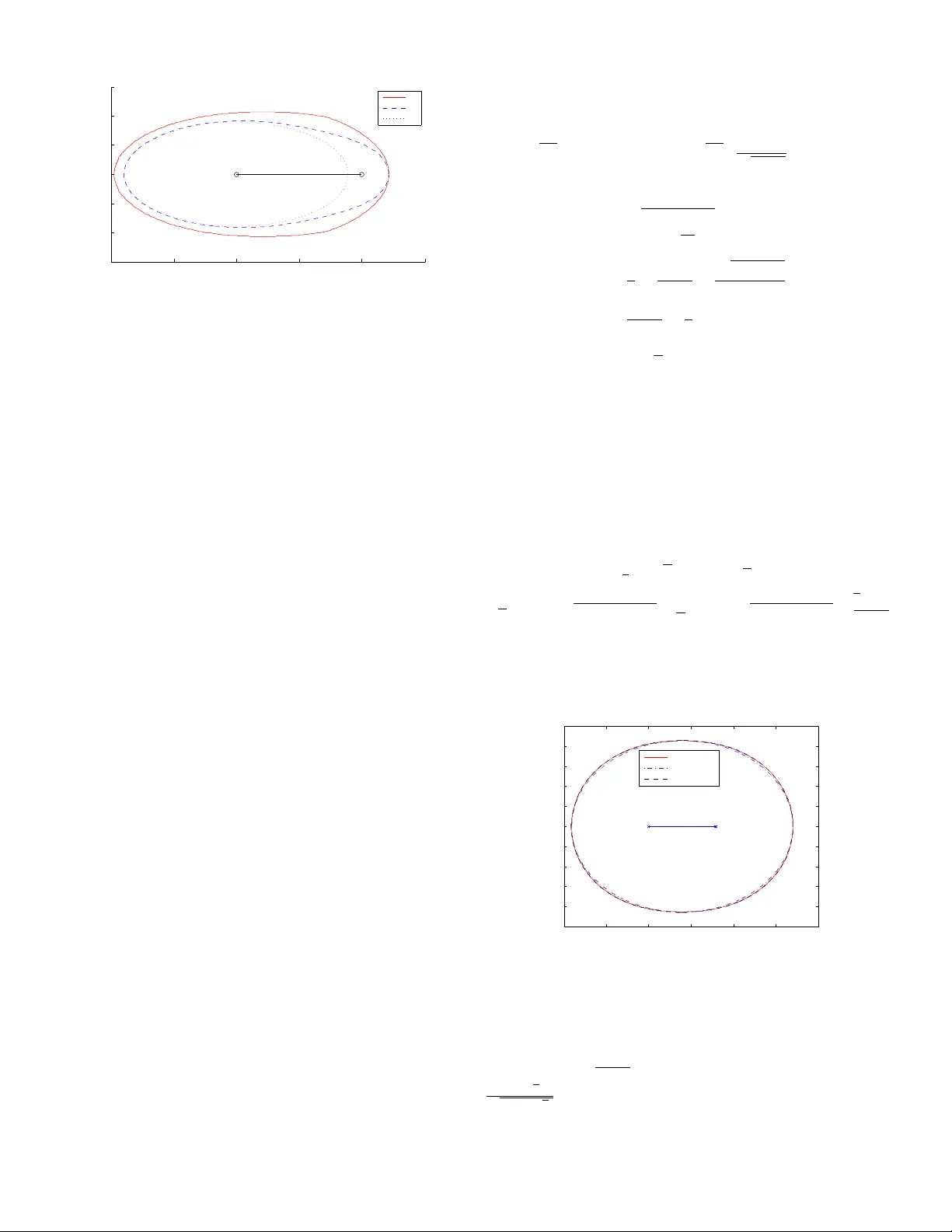
On Maximizing Co v erage in Gaussian Relay Networks V aneet Aggarwal Department of Electrical Engineering Princeton Univ ersity Email: vagg arwa@princeton.edu Amir Bennatan Program for Applied and Computational Mathematics Princeton Univ ersity Email: abn@math.princeton.edu A. Robert Calderbank Department of Electrical Engineering Princeton Univ ersity Email: calderbk@math.princeton.edu Abstract —Results for Gaussian relay channels typically focus on maximizing transmission rates for gi ven locations of the source, relay and destination. W e introduce an alternati ve per - spective, where the objective is maximizing coverage for a given rate. The new objectiv e captures the problem of how to deploy relays to pr ovide a given lev el of service to a particular geographic area, where the relay locations become a design parameter that can be optimized. W e e valuate the decode and f orward (DF) and compress and forward (CF) strategies for the relay channel with respect to the new objective of maximizing coverage. When the objective is maximizing rate, different locations of the destination fav or different strategies. When the objective is coverage for a given rate, and the relay is able to decode, DF is uniformly superior in that it pro vides coverage at any point served by CF . When the channel model is modified to include random fading, we show that the monotone ordering of coverage regions is not always maintained. While the coverage provided by DF is sensitive to changes in the location of the relay and the path loss exponent, CF exhibits a more graceful degradation with respect to such changes. The techniques used to approximate coverage regions are new and may be of independent interest. I . I N T RO D U C T I O N Relay channels ha ve recently attracted significant attention as a model for ad-hoc networks [7]. These channels model problems where one or more r elays help a pair of terminals communicate. The general channel model was first considered by v an der Meulen [1], [2], [3] and further studied in a ground breaking w ork by Cover and El Gamal [4]. Although the capacity region for the channel is still unkno wn, the results of [4] include two achie vable coding strategies which were subsequently named decode-and-forward (DF) and compress- and-forward (CF). The Gaussian relay channel was examined by Kramer et al. [5] and Høst-Madsen and Zhang [8]. A distincti ve property of the existing results in the literature is that they all consider the classic information-theoretic per- spectiv e of maximizing the achiev able rate for giv en locations of the source, relay and destination nodes. Howe ver , in many cases of practical interest, the design problem at hand is to maximize covera ge for a fixed desired transmission rate. This is the focus of our paper . The following simple e xample, illustrates the difference between the performance measure considered in this paper (maximizing coverage), and the classic measure (maximizing rate). Consider a source, relay and destination all at equal distances (say 1) from one another (on the v ertices of an equilateral triangle), as in Fig. 1. Assume equal power con- straints ( P 1 = P 2 = 1 ). Assume the requisite rate is R = 1 bits/channel use. Then DF can achiev e a maximum rate of 1 bit/channel use at the destination, yet CF can do better: 1.17. In this paper (Theorem 1, Sec. III) we assert that whenever the relay can decode, DF provides superior performance to that of CF . This example would appear to contradict that assertion. Howe ver , with the performance measure of our paper (cov erage), the advantage of CF does not matter . This is because we are not concerned with the maximum achiev able rate, as long as it is greater than R . Fig. 1. Locations of the source, the relay and the destination in the above example. In their seminal work, Kramer et al. [5][Sec. VII.B] ex- tended the classic treatment of the relay problem by consid- ering the location of the relay as a design parameter . That is, they considered the ef fect of relocating the relay on the achiev able rates at the destination. This effect is hea vily dependent on the destination’s loca- tion. While a destination at some locations may benefit from relocating the relay , a destination at other locations will suf fer . Howe v er , in many cases of practical interest, the location of the relay is determined at a time when the destination’ s location is unknown. The destination is typically a mobile station, while the relay is often a fixed terminal, whose location is determined once, at the time that the network is designed. Nev ertheless, while the location of the destination may be unknown at the time of network design, the target transmission rate is typically kno wn. Thus, the effect of changes in the relay (change of location or communication strategy) on the covera ge re gion can be ev aluated. Our analysis further extends the discussion of [5] in the following ways, 1) The discussion of [5] is limited to a single destination, at a fixed distance of 1 (normalized distance metric) from the source, and to a relay that is located on the line segment connecting the source to the destination. Our discussion is completely general. 2) In [5][Remark 31], the authors analyze the performance of DF and CF in the limit when the relay is either close to the source or close to the destination. They provide numerical data when the relay is intermediate these two extremes. In this paper, we provide rigorous analysis for all possible locations of the relay . 3) The results of [5] provide the following intuition: When- ev er the channel from the source to the relay is strong enough to enable the relay to decode the source’ s message, DF renders superior performance to that of CF . Ho wev er , re gardless of how strong (or weak) this channel may be, there is always some rate (howe ver low) that the channel can support (under the channel model both paper share). Strictly speaking, with the formulation of [5], the relay can always decode, and thus the intuition cannot be stated formally . The introduction of a target transmission rate, in this paper , enables us to formalize and prov e the intuition. W e begin in Sec. II by providing some background on the channel model and achiev able strategies for it. W e also formally define the concept of coverage. In Sec. III we compare the cov erage regions of the CF and DF achiev able strategies, for different locations of the relay . In this compari- son, we assume that the relay’ s location is the same with both strategies. W e extend the comparison in Sec IV, and allo w each strategy its o wn preferred relay location. In Sec. V we provide bounds on the area (measured in normalized units of area) of the coverage re gion of DF , as a function of the relay’ s location. The discussion in this paper mostly focuses on a full-duplex non-fading channel model. In Sec. VI we briefly discuss additional channel models. Sec. VII concludes the paper . Throughout the paper, proofs are deferred to the appendix. I I . B A C K G RO U N D A N D D E FI N I T I O N S A. The Channel Model In this section, we introduce a simple relay channel model, which will be our focus throughout most of the paper . In this model, nodes are assumed to be full-duplex. This means that a node can recei ve and transmit simultaneously . Furthermore, the signal attenuation between any two points assumed to be a deterministic function of the distance between the two. In Sec. VI we will consider additional channel models (random fading and half-duplex). Our model is depicted in Fig. 2. The channel consist of three nodes: a source (node 1), a relay (node 2) and a destination (node 3). W e consider a two-dimensional domain for our three-node network. This means that the source, relay and destination are associated with two-dimensional location vectors a 1 , a 2 and a 3 , respectiv ely . For simplicity , and without loss of generality , we may assume that a 1 = (0 , 0) , and a 2 = ( d, 0) where d > 0 is the distance between the source and the relay . The relations between the channel outputs and 12 d 23 d 13 d Source Relay Destina tio n 2 P 1 P 1 2 3 Fig. 2. Single Relay Network inputs are a function of the distances between the various nodes. W e let d kl , k , l = 1 , 2 , 3 denote the distances between nodes k and l . W ith this notation, d 12 = k a 2 k = d, d 13 = k a 3 k and d 23 = k a 3 − a 2 k where k · k denotes the Euclidean norm. See Fig. 2. The channel equations are now giv en by , y 2 [ i ] = 1 d α/ 2 12 x 1 [ i ] + z 1 [ i ] y 3 [ i ] = 1 d α/ 2 13 x 1 [ i ] + 1 d α/ 2 23 x 2 [ i ] + z 2 [ i ] where, x 1 [ i ] and x 2 [ i ] are the signals transmitted from the source and relay , respectiv ely , at time i . These signals are subject to average power constraints P 1 and P 2 , respectiv ely . y 2 [ i ] and y 3 [ i ] denote the observed signals at the relay and destination, respectiv ely . z 1 [ i ] and z 2 [ i ] are mutually indepen- dent i.i.d circularly-symmertic complex Gaussian noise with variance 1. α ≥ 2 is the path loss exponent. B. Codes and Achie vable Strate gies A code for the relay channel of rate R and block-length n , consists of a pair ( C, { f i } n i =1 ) . C is a set of 2 nR codew ords of length n . The source encoder constructs its signal by selecting a codew ord x 1 ∈ C . At time i , the source sends index x 1 [ i ] and the relay sends x 2 [ i ] using f i based on its past observation. That is, x 2 [ i ] = f i ( y 2 [ i − 1] , ..., y 2 [1]) . A relay transmission scheme S is formally a collection of relay codes. Definition 1: Gi ven locations a 2 = ( d, 0) and a 3 of the relay and the destination respectiv ely , a rate R is defined to be ac hievable by a scheme S (equiv alently: S supports R ) if for any  > 0 , there exist ( C, { f i } n i =1 ) ∈ S such that the rate of C is at least R , and the probability of error , under maximum-likelihood decoding is at most  . W e define the capacity of S at relay location a 2 = ( d, 0) and destination location a 3 as, C S ( d, a 3 ) = sup { R : S supports R } Cov er and El Gamal [4] introduced two achiev able cod- ing strategies which were subsequently named decode-and- forward (DF) and compress-and-forward (CF). W ith DF , the relay decodes the message transmitted by the source. It then cooperates with the source to transmit the message to the destination. W ith CF , the relay considers the observed signal from the source as a raw signal, compresses it, and transmits it to the destination. The destination then combines this observation with its own observation, and uses both to decode the source’ s message. An important distinction between the two strategies, is that with DF , the relay attempts to decode the source’ s message, while with CF it does not. A comprehensive description of the strategies is av ailable e.g. in [4], [5], [8]. The achie vable rates with both schemes, for our channel model, were computed in [5], [8], and are provided in Ap- pendix A. Following their example, we confine our attention to CF when the random variables used in the generation of the codebooks are Gaussian. C. Cover age W e are no w ready to formally define the concept of cover - age. Definition 2: Let R > 0 be a desired transmission rate. For a fixed distance d between the source and the relay , and a fixed transmission scheme S , we define the coverage region as, G S ( d ) ∆ = { a 3 : C S ( d, a 3 ) ≥ R } The concept of coverage is closely related to outage - we fix a target rate, and seek to maximize the geographic region, outside which an outage occurs. I I I . C O M P A R I S O N O F C F A N D D F In this section, we consider the coverage region when using the DF and CF approaches, for a fixed, giv en location of the relay a 2 . For reference, we also consider the no-r elay (NR) cov erage region, i.e, the cov erage region when the relay is not used. W e would expect dif ferent locations of the destination a 3 to fav or dif ferent schemes. That is, for a fixed rate R , some locations would be covered only by CF , others only by DF and yet others by both. Surprisingly , ho wev er , the following result indicates a monotonic ordering of the cov erage regions. Theor em 1: Assume the channel model of Sec. II and let R > 0 . Let d c be defined as follows, d c =  P 1 2 R − 1  1 /α (1) 1) If d ≤ d c , then G DF ( d ) ⊇ G CF ( d ) ⊇ G NR ( d ) 2) If d > d c , then G CF ( d ) ⊇ G NR ( d ) ⊇ G DF ( d ) = ∅ The proof is provided in Appendix B. W e now interpret the results of Theorem 1. The condition d ≤ d c determines whether the relay is still able to decode the information that is transmitted to it by the source. Whenev er the relay is able to decode, we see that DF is the method of choice. DF is uniformly superior in transmission to any point, in the sense that it provides coverage at any point served by CF . Howe ver , if the relay is not able to decode the data, then DF cannot be applied, and G DF ( d ) = ∅ . For such values of d , the best approach is CF , where the relay and destination combine their channel observations and perform collaborativ e decoding. From a design perspecti ve, while for d ≤ d c DF enjoys a larger coverage region than CF , it suffers from a sharp drop in performance when d crosses d c . In practical settings, when the path loss exponent α is not known (and consequently d c , as defined by (1), is not kno wn), this may become an important disadvantage. CF , in comparison, enjo ys a more graceful degradation with respect to changes in d . The abov e results can equi valently be stated as follows: Consider the combined transmission strategy CF ∨ DF , under which the various terminals are free to select the best of CF and DF . Theorem 1 implies that, G CF ∨ DF ( d ) =  G DF ( d ) , d ≤ d c ; G CF ( d ) , d > d c ; Figs. 3 and 4 present numerical examples of the regions considered in Theorem 1. In Fig. 3, d ≤ d c and in Fig. 4, d > d c . In both figures we also compare the cov erage regions with a region computed according to the upper -bound (UB) as provided by [5]. −1.5 −1 −0.5 0 0.5 1 1.5 2 2.5 − 1.5 −1 − 0.5 0 0.5 1 1.5 P1=10, P2=10, alpha=3.52,R=3 Source Relay UB DF CF NR Fig. 3. Coverage regions when d ≤ d c , P 1 = 10 , P 2 = 10 , α = 3 . 52 , R = 3 I V . C O M PA R I S O N W I T H U N E Q UA L R E L A Y P L AC E M E N T The analysis of Sec. III focused on coverage regions for a giv en distance d between the source and the relay . Howe ver , different schemes may fa vor different locations of the relay . Thus, in this section, we provide some interesting results that −1 −0.5 0 0.5 1 1.5 −1.5 −1 −0.5 0 0.5 1 1.5 P1=10, P2=10, alpha=3.52,R=4 Source Relay UB CF NR Fig. 4. Coverage regions when d > d c , P 1 = 10 , P 2 = 10 , α = 3 . 52 , R = 4 consider CF and DF when they are allowed differ ent locations of the relay . Theor em 2: Let R > 0 . Let d c be defined as in Theorem 1. Then the following assertions holds: 1) Assume α = 2 . Then there exists a non-negati ve positi ve fraction 0 < γ < 1 / 9 , independent of R , such that if P 2 > γ · P 1 , then for all d > d c , G CF ( d ) ⊆ G DF ( d c ) 2) There exists β ( R ) > 0 such that if P 2 < β ( R ) · P 1 , then there exists d 0 such that, G CF ( d 0 ) * [ d> 0 G DF ( d ) The proof of this theorem is provided in Appendix C Theorem 2, combined with Theorem 1, provide us with insight into the choice between strate gies DF and CF when the relay location may be optimized independently for each scheme. In the case of α = 2 , when the relay po wer is sufficiently large, DF is the method of choice regardless of the desired R . If we choose to place the relay at location d ≤ d c , then Theorem 1 tells us that G CF ( d ) ⊆ G DF ( d ) , and thus DF is superior . If d > d c , then Theorem 2 tells us that G CF ( d ) ⊆ G DF ( d c ) , and thus switching from CF and DF and repositioning the relay at d = d c would render superior performance. Regardless of α , if the power at the relay is sufficiently low , Theorem 2 tells us that there are locations and rates that may only be supported by CF . These cannot be supported by DF , regardless of where we place the relay . V . B O U N D S O N T H E D F C OV E R AG E A R E A So far , our discussion has focused on a comparison of cov erage regions with DF and CF . Howe ver , a natural question that arises is what the ar ea (in normalized units of area) of the cov erage region is, and the effect of the distance d on it. In this section we partially answer this question for the DF coverage region in a few specific cases. W e let |G DF ( d ) | denote this area, and begin with the following theorem. Theor em 3: Assume P 1 = P 2 and α = 2 . Then for all 0 < d ≤ d c , π p λγ · d 2 ≤ |G DF ( d ) | ≤ π p λγ · 1 − a/ 2 √ 1 − a · d 2 (2) where, ρ = s 1 −  d d c  2 , (3) λ = 1 4 + 1 1 − ρ + p 2(1 + ρ ) 1 − ρ 2 (4) γ = 2 1 − ρ − 1 4 (5) a = 1 − γ λ (6) Remark 1: 1) Recall, from Theorem 3, that when d > d c , G DF ( d ) = ∅ and thus |G DF ( d ) | = 0 . 2) Observe that ρ is is a function of d , and implicitly a function of of R and P 1 through its dependence on d c , which was defined by (1). Consequently , the other parameters are functions of these values too. The proof of this theorem is achie ved by bounding the cov erage region from within by an ellipse whose boundary is giv en by the points ( d 2 + √ λd cos( θ ) , √ γ d sin( θ )) , and from outside by a conic whose boundary is given by the points ( d 2 + √ λd cos( θ ) q 1 − a sin 2 ( θ ) , √ γ d sin( θ ) q 1 − a sin 2 ( θ ) / √ 1 − a ) . These two bounding shapes, for the case of P 1 = P 2 = 10 , R = 1 , are plotted in Fig. 5, along with the true re gion (computed numerically). The details of the proof are provided in Appendix D. −4 −2 0 2 4 6 8 −5 −4 −3 −2 −1 0 1 2 3 4 5 Source Relay d c Actual Area Lower Bound Upper Bound Fig. 5. Bounds for G DF , P 1 = P 2 = 10 , R = 1 , α = 2 Fig. 6 presents the bounds in (2), along with the true area (computed numerically) corresponding to the same parameters as Fig. 5. Examining this figure, we see that the bounds are very tight. By (2), the ratio between the two bounds is (1 − a/ 2) / ( √ 1 − a ) , which increases with d from 1 to 6+2 √ 2 √ 7(5+4 √ 2) ≈ 1 . 02216 . Thus, the gap between the two bounds nev er exceeds 2 . 22% . 0 0.5 1 1.5 2 2.5 3 3.5 70 80 90 100 110 120 130 d 12 Area Actual Area Lower Bound Upper Bound Fig. 6. Bounds for G DF , P 1 = P 2 = 10 , R = 1 , α = 2 Examining Fig. 6, we may observ e that |G DF ( d ) | approaches its maximum as d → 0 . T o see this, observe that both bounds coincide as d → 0 , and the upper bound decreases with d . Thus, from the point of view of maximizing coverage, the relay should optimally be placed as close to the base station as possible. While this results holds for α = 2 , it is not generally true, as the discussion below will show . The follo wing theorem extends the lower bound of (2) to the case of α = 4 . Theor em 4: Assume P 1 = P 2 and α = 4 . Then for all 0 < d ≤ d c , |G DF ( d ) | ≥ π p λγ · d 2 (7) where, ρ = s 1 −  d d c  4 (8) γ = r 2 1 − ρ − 1 / 4 (9) and λ is the largest real-valued solution of the equation,  x − 1 4  4 − 2 1 − ρ  x − 1 4  2 − 4 1 − ρ 2  x − 1 4  − 1 1 − ρ 2 = 0 (10) This solution can be found analytically by applying the Ferrari method, see e.g. [6][page 32]. The proof of this theorem follo ws along the lines of the proof of the lower bound in Theorem 3, namely by bounding the cov erage area from within by an ellipse. The details of the proof are provided in Appendix E. Fig. 7 compares the lower bound of Theorem 4 with the true area (computed numerically), when P 1 = P 2 = 100 and R = 1 . Lemma 1: The lo wer bound (7) becomes tight as d → 0 . The proof of this lemma is provided in Appendix F. Recall that with α = 2 , we proved that the maximum cov erage area was achiev ed when d → 0 . Lemma 1 enables us to sho w that this is not the case with α = 4 . T o prov e this, all we need to do is find a nonzero value of d at which the lower 0 0.5 1 1.5 2 2.5 3 3.5 56 57 58 59 60 61 62 63 64 65 d 12 Area Actual Area Lower Bound Fig. 7. Lower bound for G DF , P 1 = P 2 = 100 , R = 1 , α = 4 bound is greater than its value at d = 0 . Changing variables from d to ρ as in the proof of Lemma 1 (Appendix F), we obtain that at ρ = . 93 , |G DF | ρ = . 93 ≥ π p λγ d 2 ρ = . 93 = 2 . 0441 ..π d 2 c > 2 π d 2 c ( a ) = |G DF ( d = 0) | where (a) follows as in the proof of Lemma 1. V I . A D D I T I O NA L C H A N N E L M O D E L S A. Half Duple x Relay The half-duplex relay model is characterized by a relay that cannot transmit and recei ve at the same time. A comprehensi ve discussion of this case is provided in [9], [5] and [10]. In this setting, we assume that there exists a positi ve fraction t ∈ [0 , 1] such that the relay is listening (recei ving) during a proportion t of the time, and transmitting during a proportion 1 − t of the time. For this setting, we have the following theorem, Theor em 5: Assume the half-duplex channel model and let R > 0 . The follo wing results hold. 1) If t = 1 / 2 and d < d 0 c , where d 0 c =  P 1 2 2 R − 1  1 /α (11) then G DF ( d ) ⊇ G CF ( d ) ⊇ G NR ( d ) 2) If d > d c , then for all t ∈ [0 , 1] G CF ( d ) ⊇ G NR ( d ) ⊇ G DF ( d ) The proof is provided in Appendix G. This theorem is weaker than Theorem 1, because d 0 c < d c . Furthermore, note that we hav e confined our attention to the case that t = 1 / 2 . B. Random F ading Models In this section, we modify the channel model of Sec. II to introduce some random fading. The new channel equations are now giv en by , y 2 [ i ] = h 12 d α/ 2 12 e j ϕ 12 [ i ] x 1 [ i ] + z 1 [ i ] y 3 [ i ] = h 13 d α/ 2 13 e j ϕ 13 [ i ] x 1 [ i ] + h 23 d α/ 2 23 e j ϕ 23 [ i ] x 2 [ i ] + z 2 [ i ] W e consider two fading models, 1) Phase fading h kl = 1 for all { k,l } . ϕ kl [ i ] are uniformly distributed ov er [0 , 2 π ) , and are jointly independent of one other , of the transmitted signals and the noise. Their time realizations are also independent. 2) Rayleigh fading. ϕ kl [ i ] is defined as in the phase fading case. h kl are Rayleigh distrib uted with parameter 1, independent, and remain fixed for the duration of the transmission. In all cases, we assume that the realizations of the random variables h kl and ϕ kl [ i ] are known to the recei vers but not to the transmitters. W e begin by considering the phase-fading model. In Ap- pendix H-A we will show that Theorem 1 carries over directly to this case. Furthermore, Kramer et al. [5] hav e computed an upper bound (UB) on the capacity in the phase-fading model. In Appendix H-B we prov e the following lemma. Lemma 2: Assume d ≤ d c where d c is giv en by (1). Then G UB ( d ) = G DF ( d ) . W e now proceed to provide some interesting observ ation for the Rayleigh fading model. This channel is no longer an ergodic channel, and thus we redefine the coverage region in terms of outage pr obabilities ([7], [5]). Definition 3: Let R > 0 be a desired transmission rate and 0 <  < 1 be the maximum tolerable outage probability . For a fixed distance d between the source and the relay , and a fixed transmission scheme S , we define the coverage region as, G S ( d ) ∆ = { a 3 : P r [ C S ( d, a 3 ) ≥ R ] ≥ 1 −  } W e define ˆ d c in a manner analogous to d c of Theorem 1, ˆ d c =  − P 1 ln(1 −  ) 2 R − 1  1 /α ˆ d c is the distance after which the relay cannot decode with probability greater than 1 −  . At relay locations satisfying d > ˆ d c , DF cannot be applied. Expressions for the achie vable rates with CF and DF in this case are av ailable in [5]. In Fig. 8 we hav e plotted the coverage regions for the various schemes in the Rayleigh fading model. Interestingly , the monotonic ordering of G CF ( d ) and G DF ( d ) , which was observed in Theorem 1 for the simple (non-fading) model, is not maintained. Neither of the two regions contains the other . −1.5 −1 −0.5 0 0.5 1 1.5 2 −1.5 −1 −0.5 0 0.5 1 1.5 Source Relay UB DF NR CF Fig. 8. Coverage regions with Rayleigh Fading and d < ˆ d c , P 1 = 3 , P 2 = 0 . 3 , α = 3 . 52 , R = 1 ,  = 0 . 35 , d = 0 . 9 V I I . C O N C L U S I O N In this paper , we have introduced a new perspectiv e on the relay channel, switching from maximizing rate at a fixed gi ven destination location, to maximizing cov erage for a given rate. This perspecti ve opens up an array of ne w possibilities for research. Our main contrib utions are first, the formulation of the problem in Sec. II. In Theorem 1, we hav e obtained the surprising result that for any given placement of the relay , one of the two common strategies (CF and DF) is uniformly optimal, and thus a relay that switches between the two is not required. Theorem 2 extends the comparison for the case of α = 2 by allo wing each of the strategies its own preferred relay location. In this case, it is interesting that the results depend on the power constraint on the relay . Theorems 1 and 2 imply that while DF often provides a larger cov erage region than CF , it is also more sensitive to changes in the location of the relay and the path loss exponent α . In contrast, CF is more robust and pro vides a more graceful de gradation with respect to such changes. A natural question that arises, when considering co verage regions, is the numeric area of the region, as a function of the distance between the source and the relay . In Sec. V we hav e provided bounds in two special cases. In Sec.VI, we hav e hav e extended our discussion to half- duplex and random-fading channel models. In particular , our results for fading channels indicate that the monotonic order- ing of the DF and CF coverage regions no longer holds. A further study of the ef fect of relocating the relay , in such settings, is of great practical interest. In this paper , we hav e focused on a one-relay setting. An interesting extension would consider two or more relays. In this case, the number of degrees of freedom grows substan- tially , as not only distance to the relays but also the angles between the line segments connecting them to the source, may be optimized. An analysis of the benefit from cooperation between the relays, is also of great interest. A P P E N D I X A G E N E R A L E X P R E S S I O N S A N D N OTA T I O N A. DF and CF Achie vable Rates The achiev able rates, with DF and CF , that were computed by [5], [8], C DF = max 0 ≤ ρ ≤ 1 min  log  1 + P 1 d α 12 (1 − ρ 2 )  , log 1 + P 1 d α 13 + P 2 d α 23 + 2 ρ √ P 1 P 2 d α/ 2 13 d α/ 2 23 !) (12) C CF = log 1 + P 1 d α 12 (1 + ˆ N 2 ) + P 1 d α 13 ! (13) where ˆ N 2 is giv en by , ˆ N 2 = P 1 (1 /d α 12 + 1 /d α 13 ) + 1 P 2 /d α 23 (14) B. Switch to P olar Coordinates W e frequently use the polar coordinates x and θ to parame- terize the destination’ s location, i.e. we assume the destination is placed at, a 3 = ( x cos θ , x sin θ ) (15) Letting d denote the distance between the source and the relay , the distances d 12 , d 13 and d 23 (see Sec. II-A) now satisfy , d 12 = d , d 13 = x , and d 2 23 = d 2 + x 2 − 2 dx cos θ . A P P E N D I X B P RO O F O F T H E O R E M 1 W e begin by noting that for all d > 0 , the result G CF ( d ) ⊇ G NR ( d ) is straightforward from (13) and from the observ ation that, C NR = log  1 + P 1 d α 13  (16) W e now prove Part 2 of the theorem, which is the easier of the two parts. Whenever d > d c , by (1), R > log  1 + P 1 d α  = max ρ ∈ [0 , 1] log  1 + P 1 d α (1 − ρ 2 )  > C DF where the last inequality was obtained by (12), recalling that d 12 = d . This is true reg ardless of the destination location a 3 , and thus DF cannot support a rate of R anywhere and G DF ( d ) = φ . Before proceeding to the proof of Part 1 of the theorem, we introduce the following notation. For a given scheme S ( S being DF or CF), and a given θ , we define x S ( θ ) as the maximum x such that a destination with polar coordinates ( x, θ ) (see Appendix A) is contained in G S ( d ) . The proof now focuses on showing that x DF ( θ ) ≥ x CF ( θ ) for all θ . By (12), we may obtain a lower bound on C DF by restricting the maximization to ρ = 0 . Thus, C DF ≥ min  log  1 + P 1 d α 12  , log  1 + P 1 d α 13 + P 2 d α 23  (17) The follo wing lemma e xamines this expression at x = x DF ( θ ) . Lemma 3: For all θ , consider the point a 3 whose polar coordinates are giv en by ( θ, x DF ( θ )) . Then the follo wing holds at a 3 , P 1 d α 12 > P 1 d α 13 + P 2 d α 23 (18) Pr oof: Assume, by contradiction, that (18) does not hold. Letting x = x DF ( θ ) , we will now show that we may increase x and preserve C DF ≥ R , contradicting the maximality of x DF ( θ ) . Consider (12). Whenev er (18) does not hold, we have, for all ρ , log  1 + P 1 d α 12 (1 − ρ 2 )  ≤ log  1 + P 1 d α 12  < log 1 + P 1 d α 13 + P 2 d α 23 + 2 ρ √ P 1 P 2 d α/ 2 13 d α/ 2 23 ! Thus, the minimization in (12) is achie ved by the first term. Changing x does not affect this term. Increasing x affects d 13 and d 23 and thus reduces the second term. Ho we ver , by a continuity argument, we may increase x slightly without altering the in v alidity of (12). Thus, the minimization in (12) would still be achiev ed by the first term, and C DF will not change. Therefore, if C DF ≥ R at x = x DF ( θ ) , it will remain so after we increase x a little, producing the desired contradiction. By Lemma 3, (17) implies that at x = x DF ( θ ) , C DF ≥ log  1 + P 1 d α 13 + P 2 d α 23  (19) > C CF (20) The last inequality may be obtained by simple arithmetic using (13) and (14). By a continuity argument, C DF = R at ( θ, x DF ( θ )) , and thus the abo ve inequality implies that C CF < R at this point. W e now argue that this result implies that G DF ( d ) ⊇ G CF ( d ) . This would follow if we could show that C CF decreases in the range x > x DF ( θ ) , for all θ . In the range x > d , d 13 , d 23 can easily be sho wn to be increasing functions. This implies that ˆ N 2 increases (see (14)), and consequently C CF decreases (see (13)). Thus, our desired result would now follo w if we could prove that x DF ( θ ) > d for all θ . T o see this, observe that by (16) and (1), G NR is a sphere with radius d c . W e ha ve shown that G NR ⊂ G CF . Thus, if C CF < R at ( θ , x DF ( θ )) (as we ha ve sho wn above), then x DF ( θ ) ≥ d c ≥ d (the last inequality being one of the conditions of this part of the theorem). This is precisely the result we sought, thus completing the proof of Part 1 of the theorem. A P P E N D I X C P RO O F O F T H E O R E M 2 Before beginning with the proof, we argue that we may assume, without loss of generality , that P 1 (the po wer of the source) is 1. T o see this, observ e that if P 1 6 = 1 , we may replace P 1 and P 2 by ˆ P 1 = 1 and ˆ P 2 = P 2 /P 1 . This substitution preserves the ratio ˆ P 1 / ˆ P 2 = P 1 /P 2 , and has the effect of scaling the DF and CF cov erage regions. That is, if we relocate the relay and the destination from any locations a 2 and a 3 (respectiv ely) to 1 /P 1 /α 1 · a 2 and 1 /P 1 /α 1 · a 3 , the achiev able rates C CF and C DF would remain unchanged. Under these assumptions, gi ven that the relay is placed at ( d, 0) , and using the notation of Sec. A, the expressions for the DF and CF achiev able rates (12) and (13) may be rewritten as, C DF = max 0 ≤ ρ ≤ 1 min  log  1 + 1 d α (1 − ρ 2 )  , log 1 + 1 x α + P 2 d α 23 + 2 ρ √ P 2 d α/ 2 d α/ 2 23 !) (21) C CF = log 1 + 1 d α (1 + ˆ N 2 ) + 1 x α ! (22) and (14) by , ˆ N 2 = 1 /d α + 1 /x α + 1 P 2 /d α 23 (23) A. Pr oof of P art 1 of Theorem 2 In this section, we assume that α = 2 . Rather than focus on C DF and C CF as in (21) and (22), the follo wing lemma allows us to rev ert to two alternati ve functions. Lemma 4: Let C DF ( x, θ , d ) and C CF ( x, θ , d ) denote the achiev able rates when the relay is placed at ( d, 0) and the destination location is deriv ed from x and θ . Let, ˜ C DF ( x, θ ) ∆ = log 1 + 1 x 2 + P 2 d 2 23 ,c ! (24) C + CF ( x, θ ) ∆ = log   1 + 1 x 2 + P 2 inf d > d c ( P 2 d 2 + d 2 23 )   (25) where d 23 ,c is the distance from a relay placed at ( d c , 0) to the destination, and d 23 is the same for a relay placed at ( d, 0) . Then the following holds: 1) ˜ C DF ( x, θ ) ≥ R if and only if C DF ( x, θ , d c ) ≥ R . Equiv alently , G DF ( d c ) = n ( x cos θ , x sin θ ) : ˜ C DF ( x, θ ) ≥ R o 2) C + CF ( x, θ ) upper bounds C CF ( x, θ , d ) for all d ≥ d c , and therefore, [ d ≥ d c G CF ( d ) ⊂  ( x cos θ , x sin θ ) : C + CF ( x, θ ) ≥ R  Pr oof: Part 1 follows from the observation that when d = d c , by (1), any choice of ρ in (21) other than ρ = 0 would render C DF < R . Part 2 follows by bounding the term d 2 (1 + ˆ N 2 ) , which appears in (22), d 2 (1 + ˆ N 2 ) = d 2 (1 /d 2 + 1 /x α + 1 + P 2 /d 2 23 ) P 2 /d 2 23 ≥ d 2 d 2 23 (1 /d 2 + P 2 /d 2 23 ) P 2 = d 2 23 + P 2 d 2 P 2 Our aim now is to show that wherev er C + CF ( x, θ ) ≥ R , also ˜ C DF ( x, θ ) ≥ R . In the sequel, we use the shorthand notation s ∆ = cos θ . Lemma 5: Let θ be fixed, 1) If s ≤ 0 , then for all x > 0 , ˜ C DF ( x, θ ) ≥ C + CF ( x, θ ) . 2) Assume s > 0 and let x 1 be giv en by , x 1 = 1 s √ P 2 + 1 √ P 2 + 1 − √ P 2 · d c (26) Then the following holds, C + CF ( x, θ ) ≤ ˜ C DF (min( x, x 1 ) , θ ) Pr oof: Observe, by (24) and (25) that ˜ C DF ( x, θ ) ≥ C + CF ( x, θ ) if and only if f min ≥ d 23 ,c 2 where f min is given by , f min = inf d ≥ d c ( P 2 d 2 + d 2 23 ) (27) Let f ( d ) be defined by , f ( d ) ∆ = P 2 d 2 + d 2 23 = ( P 2 + 1) d 2 + x 2 − 2 dxs (28) where the last equality was obtained by the cosine theorem. T aking the deri vati ve of f ( d ) , we obtain that the unconstrained minimum (i.e., the minimum in the range d ∈ ( −∞ , ∞ ) ) is obtained at, d min = xs P 2 + 1 (29) If s ≤ 0 then d min ≤ 0 < d c , and thus f min , which is the minimum in the range d ≥ d c , is obtained at d c . Thus, f min = f ( d c ) = P 2 d 2 c + d 2 23 ,c > d 2 23 ,c , and our desired result of Part 1 of the lemma follows. T o pro ve Part 2, we begin by considering the range x ∈ [0 , x 1 ] . W e further divide the interval x ∈ [0 , x 1 ] into two ov erlapping intervals, [0 , x 0 ] and [ x 00 , x 1 ] and prove the desired result separately in each interval. W e define, x 0 = 1 s · d c x 00 = 1 s √ P 2 + 1 √ P 2 + 1 + √ P 2 · d c Clearly , x 00 < x 0 < x 1 , and thus the two intervals ov erlap. If x ≤ x 0 then d min < d c (by (29)), and thus f min ≥ d 2 23 ,c as in the proof of Part 1 of the lemma. Thus, the desired result is obtained for x ∈ [0 , x 0 ] . W e proceed to consider the interv al x ∈ [ x 00 , x 1 ] . The minimum f min (constrained to d ≥ d c ) clearly satisfies f min ≥ f ( d min ) . By (28) and (29), we ha ve, after some algebraic manipulations, f ( d min ) = x 2  1 − s 2 P 2 + 1  (30) Thus, a sufficient condition for f min ≥ d 2 23 ,c is, x 2  1 − s 2 P 2 + 1  ≥ d 2 23 ,c (31) Applying the cosine theorem and rearranging the terms, we obtain the inequality , s 2 P 2 + 1 · x 2 − (2 d c s ) x + d 2 c ≤ 0 (32) The left hand side of this inequality is a parabola in x , whose roots are x 00 and x 1 . Thus, the inequality is satisfied for all x ∈ [ x 00 , x 1 ] . Consequently , by the above discussion, f min ≥ d 2 23 ,c in this interval, as desired. This completes the proof on the lemma in the interval x ∈ [0 , x 1 ] . Before proceeding to the interval [ x 1 , ∞ ) , observe that x 1 satisfies (32) and consequently (31), with equality . Equi va- lently , x 2 1  1 − s 2 P 2 + 1  = d 2 23 ,c (33) W e now consider x ≥ x 1 . Observe that the discussion leading to (30) remains valid in this range. By (25), C + CF ( x, θ ) = log   1 + 1 x 2 + P 2 inf d > d c ( f ( d, x, θ )   ≤ log   1 + 1 x 2 + P 2 inf d > 0 f ( d, x, θ )   ( a ) = log   1 + 1 x 2 + P 2 x 2  1 − s 2 P 2 +1    ( b ) ≤ log   1 + 1 x 2 1 + P 2 x 2 1  1 − s 2 P 2 +1    ( c ) = log 1 + 1 x 2 1 + P 2 d 2 23 ,c ! = ˜ C DF ( x 1 , θ ) where (a) is obtained by (30), (b) follows from x ≥ x 1 , and (c) is obtained by (33). Lemmas 4 and 5 imply that a sufficient condition for Part 1 of Theorem 2 is ˜ C DF ( x 1 , θ ) ≤ R for all θ such that s = cos θ > 0 (recall that x 1 is a function of θ ) and all P 2 > 1 / 9 (recall that we hav e assumed that P 1 = 1 ). Using (1) and (24), ˜ C DF ( x 1 , θ ) ≤ R can be rewritten as, log 1 + P 2 d 2 23 ,c + 1 x 2 1 ! ≤ log  1 + 1 d 2 c  (34) W e now introduce the notations, A = 1 s √ P 2 + 1 √ P 2 + 1 − √ P 2 , B =  1 − s 2 P 2 + 1  (35) Observe that A and B are functions of s . With these notations, using (26) and (33), we obtain, x 1 = A · d c and d 2 23 ,c = B x 2 1 = B A 2 · d 2 c . Plugging these identities into (34), with some algebraic manipulations, leads to the inequality , P 2 ≤ B ( A 2 − 1) (36) The right hand side of the abov e inequality is a descending function of s in the range s ∈ [0 , 1] . Thus, a necessary and sufficient condition for the inequality to be valid for all s ∈ [0 , 1] is that the inequalities hold for s = 1 . W e thus confine our attention to this case. Using (35), we may rewrite (36) as, P 2 ≤  1 − 1 P 2 + 1  "  √ P 2 + 1 √ P 2 + 1 − √ P 2  2 − 1 # W e now proceed to develop this inequality , P 2 ≤ P 2 P 2 + 1  P 2 + 1 ( √ P 2 + 1 − √ P 2 ) 2 − 1  ( p P 2 + 1 − p P 2 ) 2 ( a ) ≤ P 2 + 1 P 2 + 2 p P 2 + 1 − p P 2 ( b ) ≤ √ P 2 + 1 √ P 2 + 2 p ( P 2 + 1)( P 2 + 2) ( c ) ≤ p P 2 ( P 2 + 2) + p P 2 + 1 ( P 2 + 1)( P 2 + 2) ( d ) ≤ P 2 ( P 2 + 2) + P 2 + 1 + +2 p P 2 ( P 2 + 2)( P 2 + 1) 1 ≤ 2 p P 2 ( P 2 + 2)( P 2 + 1) 1 4 ( e ) ≤ P 2 ( P 2 + 2)( P 2 + 1) (37) (a) is obtained by multiplying both sides by ( P 2 + 1) /P 2 · ( √ P 2 + 1 − √ P 2 ) 2 . (b) is obtained by taking the square root of both sides. (c) is obtained by multiplying both sides by √ P 2 + 2 and rearranging terms. (d) is obtained by taking the squares of both sides. (e) is obtained by dividing by 2 and taking the square of both sides. Finally , the right hand side of (37) is an ascending function of P 2 . The inequality can be verified to be satisfied for P 2 = 1 / 9 , and thus it is satisfied for all P 2 > 1 / 9 . B. Pr oof of P art 2 of Theorem 2 W e be gin with an outline of the proof. The proof follo ws from the observation that regardless of how low the power at the relay may be, if the destination is close enough to the relay , then arbitrarily high reliability may be achie ved in the link between them. With CF , the relay and the destination cooperate and form a virtual antenna array . W ith DF , the relay must decode alone, and is thus confined to the no-relay cov erage region (i.e., d must not exceed d c ). If its power is suf ficiently low , it cannot service a destination that is beyond the no-relay region. W e confine our attention in this section to destinations a 2 of the form (0 , x ) where x > d c . W e begin by examining C DF . By (21) (assuming, as discussed abov e, that P 1 = 1 ), lim sup P 2 → 0 C DF ≤ lim P 2 → 0 max 0 ≤ ρ ≤ 1 log 1 + 1 x α + P 2 d α 23 + 2 ρ √ P 2 x α/ 2 d α/ 2 23 ! = log  1 + 1 x α  < log  1 + 1 d α c  = R The last equality follows by (1). Thus, at any x > d c , for P 2 that is too small, C DF < R , and thus we may not support the desired rate of R . W e no w turn to examine C CF . W e wish to find a destination location a 3 = (0 , x ) , where x > d c , such that regardless of how low the relay po wer P 2 may be, by positioning the relay close enough to the destination, we will be able to support the desired rate of R . Combining this with our above result for DF will conclude the proof. Let x > d c be arbitrary . W e will examine relay locations giv en by (0 , d ) , where d = x − P 1 /α 2 . W ith this choice, P 2 /d α 23 = 1 . lim P 2 → 0 C CF = lim P 2 → 0 log 1 + 1 d α (1 + ˆ N 2 ) + 1 x α ! Where we ha ve used d 12 = d , and d 13 = x . Now , it is straightforward to verify that the following holds, recalling that d is now a function of P 2 , and it satisfies P 2 /d α 23 = 1 . lim P 2 → 0 d α (1 + ˆ N 2 ) = 2(1 + x α ) Thus, lim P 2 → 0 C CF = log  1 + 1 2(1 + x α ) + 1 x α  Now , taking the limit as x → d c , we obtain: lim x → d c  lim P 2 → 0 C CF  = log  1 + 1 2(1 + d α c ) + 1 d α c  > log  1 + 1 d α c  = R where the last equality follows by (1). Thus, there exists x 0 > d c , such that for arbitrarily small P 2 , the achiev able rate with CF (when the relay is appropriately placed) is greater than R . This is exactly what we set out to prov e, thus concluding the proof of the theorem. A P P E N D I X D P RO O F O F T H E O R E M 3 A. The Lower Bound As noted in Section V, the proof of the lower bound follows by bounding the coverage region from within by an ellipse whose boundary is giv en by the points,  d 2 + √ λd cos( θ ) , √ γ d sin( θ )  (38) W e let A denote this ellipse. W e be gin by focusing on the boundary of A , and sho w that it lies within the DF coverage region. W e will later show that this implies that interior of A is contained in the cov erage region as well. W e must therefore show that at each point a 3 on the boundary of A , C DF ( P 2 = P 1 , α = 2) ≥ R (39) where C DF is giv en by (12). Note that by (38), at a point on the boundary of A , the following holds, d 2 13 = d 2  ( 1 2 + √ λ cos( θ )) 2 + ( √ γ sin( θ )) 2  (40) d 2 23 = d 2  ( 1 2 − √ λ cos( θ )) 2 + ( √ γ sin( θ )) 2  (41) Consider (12). It is easy to observe that whenev er C DF is greater or equal to R , then selecting ρ to coincide with (3) would at worst reduce C DF to equal R . This is because this choice renders the first minimization term equal to R and can only increase the second term. Thus, we assume, without loss of generality , that this value of ρ maximizes (12). Thus, proving (39) is equiv alent to proving (recall that P 1 = P 2 ), log  1 + P 1 d 2 13 + P 1 d 2 23 + 2 ρP 1 d 13 d 23  ≥ R = log  1 + P 1 d 2 12 (1 − ρ 2 )  . Substituting (40) and (41) into the above equations, after some manipulations, we get (42) at the top of the page. W e now define s ∆ = sin 2 ( θ ) . W e also define, t ( s ) ∆ = 1 4 + λ − ( λ − γ ) s (43) f ( s ) ∆ = t 2 ( s ) − λ + λs (44) Using this, equation (42) reduces to 2 t ( s ) f ( s ) + 2 ρ p f ( s ) − (1 − ρ 2 ) ≥ 0 . W e will soon show (Lemma 6) that f ( s ) > 0 , and thus, multiplying abov e equation by − f ( s ) , we obtain that it is enough to show that h ( s ) ∆ = − 2 t ( s ) − 2 ρ p f ( s ) + (1 − ρ 2 ) f ( s ) ≤ 0 , for all s ∈ [0 , 1] . W e will soon show (Lemma 7) that h ( s ) is zero on the end points of the interv al s ∈ [0 , 1] ; hence it is enough to prov e that h ( s ) is conv ex. This will soon be proved in Lemma 8. The above discussion implies that the boundary of A lies within G DF . W e now ar gue that this implies that the interior of A is contained in G DF as well. Consider a point a 3 in the interior of A , and consider its polar coordinates (15). If x ≤ d , then it can easily be observed from (13) that C DF ≥ R (recall that d 13 = x, d 12 = d and that we have assumed d ≤ d c ). No w , keeping θ fixed, consider the range { x : d < x < x A ( θ ) } , where x A ( θ ) lies on the boundary of A . Both d 13 and d 23 can easily be shown to be ascending functions of x in this 1 ( 1 2 + √ λ cos( θ )) 2 + ( √ γ sin( θ )) 2 + 1 ( 1 2 − √ λ cos( θ )) 2 + ( √ γ sin( θ )) 2 + 2 ρ q (( 1 2 + √ λ cos( θ )) 2 + ( √ γ sin( θ )) 2 ) 1 q (( 1 2 − √ λ cos( θ )) 2 + ( √ γ sin( θ )) 2 ) ≥ 1 − ρ 2 (42) range, and thus by (12), C DF is a descending function of x . Therefore, if C DF ≥ R at the boundary point x A ( θ ) , then it is greater than R at any point satisfying x < x A ( θ ) . W e no w prove some of the lemmas that were used in the abov e discussion. Lemma 6: 1) λ − γ ≥ 1 2 2) t 0 ( s ) < 0 for all s ∈ [0 , 1] 3) f ( s ) is con vex 4) f 0 ( s ) ≤ 0 for all s ∈ [0 , 1] 5) f ( s ) ≥ 4 (1 − ρ ) 2 > 0 for all s ∈ [0 , 1] Pr oof: 1) λ − γ − 1 2 = 1 4 + 1 1 − ρ + p 2(1 + ρ ) 1 − ρ 2 − 2 1 − ρ + 1 4 − 1 2 = p 2(1 + ρ ) − (1 + ρ ) 1 − ρ 2 = √ 1 + ρ 1 − ρ 2 ( √ 2 − p 1 + ρ ) ≥ 0 2) t 0 ( s ) = − ( λ − γ ) < 0 by Part (1) of this Lemma. 3) f 00 ( s ) = 2 t 0 2 ( s ) = 2( λ − γ ) 2 > 0 by Part (1) of this Lemma. 4) f 0 ( s ) = 2 t ( s )( γ − λ ) + λ . As t ( s ) is decreasing function (part (2) of this lemma), we need to prove that 2 t (1)( γ − λ ) + λ ≤ 0 , or 2( 1 4 + γ )( λ − γ ) ≥ λ . Or , 2  2 1 − ρ  1 2 − 1 1 − ρ + p 2(1 + ρ ) 1 − ρ 2 ! ≥ 1 4 + 1 1 − ρ + p 2(1 + ρ ) 1 − ρ 2 After some manipulations, this is equiv alent to proving (3 + ρ )  r 2 1 + ρ + 1 − ρ 4  ≥ 4 which is true since the left hand side decreases with ρ ∈ [0 , 1) and goes to 4 as ρ → 1 . 5) As f 0 ( s ) ≤ 0 (by pre vious part of this Lemma), f ( s ) ≥ f (1) = t 2 (1) = 4 (1 − ρ ) 2 . Lemma 7: h ( s ) = 0 on the end points of the interval s ∈ [0 , 1] , that is 1) h (0) = 0 2) h (1) = 0 Pr oof: 1) h (0) = − 2 t (0) − 2 ρ p f (0) + (1 − ρ 2 ) f (0) = − 2  1 4 + λ  − 2 ρ  λ − 1 4  +(1 − ρ 2 )  λ − 1 4  2 = − 2 1 2 + 1 1 − ρ + p 2(1 + ρ ) 1 − ρ 2 ! − 2 ρ 1 1 − ρ + p 2(1 + ρ ) 1 − ρ 2 ! +(1 − ρ 2 ) 1 1 − ρ + p 2(1 + ρ ) 1 − ρ 2 ! 2 = − 2 1 2 + 1 + ρ 1 − ρ + p 2(1 + ρ ) 1 − ρ ! + 1 + ρ 1 − ρ 1 + 2 1 + ρ + 2 p 2(1 + ρ ) 1 + ρ ! = − 1 − 1 + ρ 1 − ρ + 2 1 − ρ = 0 2) h (1) = − 2 t (1) − 2 ρ p f (1) + (1 − ρ 2 ) f (1) = − 2  1 4 + γ  − 2 ρ  1 4 + γ  +(1 − ρ 2 )  1 4 + γ  2 = (1 / 4 + γ )( − 2 − 2 ρ + (1 − ρ 2 )  2 1 − ρ  ) = 0 Lemma 8: h ( s ) is con vex. Pr oof: h ( s ) ∆ = − 2 t ( s ) − 2 ρ p f ( s ) + (1 − ρ 2 ) f ( s ) . Since t ( s ) is linear , it is enough to show that − 2 ρ p f ( s ) + (1 − ρ 2 ) f ( s ) is con vex. Let g ( x ) ∆ = − 2 ρ √ x + (1 − ρ 2 ) x, for x > 0 , we need to show g ( f ( s )) is con vex. Since f ( s ) is con vex (Lemma 6), g ( x ) is con vex in the range { x : x > 0 } (this is easily obeerved by , g 00 ( x ) = ρ 2 x − 3 / 2 > 0 ), it is enough to show that g ( x ) is non-decreasing in its domain, and by a well-known con vex analysis result (see, e.g. [11][Page 85]) we will obtain that h ( s ) is con vex. T o show that g ( x ) is non-decreasing in its domain, we see that g 0 ( x ) ≥ 0 when x ≥  ρ 1 − ρ  2 . Since f ( x ) ≥ 4 (1 − ρ ) 2 ≥  ρ 1 − ρ  2 by Lemma 6, g ( x ) is non-decreasing in the range of f ( x ) . B. The Upper Bound As noted in Section V, the proof of the upper bound follows by bounding the co verage region from outside by a conic whose boundary is giv en by the points,  d 2 + √ λd cos( θ ) q 1 − a sin 2 ( θ ) , √ γ d sin( θ ) q 1 − a sin 2 ( θ ) √ 1 − a   (45) W e let B denote this conic. The proof follows along lines similar to those of Appendix D-A. Once again, we be gin by focusing on the boundary of the conic B , and show that on every point on this, C DF ≤ R . W e will later sho w that this implies that exterior of the conic is not contained in the cov erage region either . W e must therefore show that at each point a 3 on the boundary of B , C DF ( P 2 = P 1 , α = 2) ≤ R (46) where C DF is giv en by (12). Note that at a point (45) the boundary of B , the following holds, d 2 13 = d 2 "  1 2 + √ λ cos( θ ) q 1 − a sin 2 ( θ )  2 +   √ γ sin( θ ) q 1 − a sin 2 ( θ ) √ 1 − a   2    (47) d 2 23 = d 2 "  1 2 − √ λ cos( θ ) q 1 − a sin 2 ( θ )  2 +   √ γ sin( θ ) q 1 − a sin 2 ( θ ) √ 1 − a   2    (48) As in Appendix D-A, we may assume without loss of generality that ρ in (12) is gi ven by (3). W ith this choice, (46) becomes (recalling P 1 = P 2 ), log  1 + P 1 d 2 13 + P 1 d 2 23 + 2 ρP 1 d 13 d 23  ≤ R = log  1 + P 1 d 2 12 (1 − ρ 2 )  . Substituting (47) and (48) into this equation, we get, after some manipulations, (46) becomes (49) at the top of the page. W e now define s ∆ = sin 2 ( θ ) , t ( s ) ∆ = 1 4 + λ (1 − as ) and f ( s ) ∆ = t 2 ( s ) − λ (1 − s )(1 − as ) . W ith this notation, (49) becomes, 2 t ( s ) f ( s ) + 2 ρ p f ( s ) − (1 − ρ 2 ) ≤ 0 . W e will soon show (Lemma 9) that f ( s ) > 0 , and thus, multiplying abov e equation by f ( s ) / 2 , we obtain that it is enough to show that h ( s ) ∆ = t ( s ) + ρ p f ( s ) − 1 − ρ 2 2 f ( s ) ≤ 0 for all s ∈ [0 , 1] . W e will soon sho w (Lemma 10) that h ( s ) = 0 on the end points of the interv al s ∈ [0 , 1] ; hence it is enough to prov e that h ( s ) is con ve x which will follow from Lemma 10. The abov e discussion implies that the boundary of B , C DF ≤ R , with C DF = R only when sin 2 θ = 0 or 1 . W e no w argue that this implies that the exterior of B lies outside G DF . The discussion follo ws closely in the lines of a similar discussion in Appendix D-A. Consider an arbitrary point a 3 , and consider its polar coordinates (15). W e also let x B ( θ ) denote the value of x that coincides with the boundary of B (45). For all, x ≤ d , we have, as in Appendix D-A, C DF ≥ R . For θ such that s = sin 2 θ / ∈ { 0 , 1 } , we hav e shown above that C DF < R , and so x B ( θ ) > d . At the other values of θ , this can be shown by direct analytic calculation using (45). In the range x > d , C DF can be sho wn to be strictly descending (as in Appendix D-A). Using our results for the boundary of B , namely that C DF ≤ R when x = x B ( θ ) , we obtain that for all x > x B ( θ ) , C DF < R , and thus all such points (which constitute the exterior of B ) lie outside of G DF . W e now prov e some results that were required in the above discussion. Lemma 9: 1) λ − γ ≤ 1 2) f 00 ( s ) ≤ 0 3) f 0 ( s ) ≤ 0 4) f ( s ) > 0 Pr oof: 1) λ − γ − 1 = 1 4 + 1 1 − ρ + p 2(1 + ρ ) 1 − ρ 2 − 2 1 − ρ + 1 4 − 1 = 2 p 2(1 + ρ ) − 2(1 + ρ ) − 1 + ρ 2 2(1 − ρ 2 ) = 2 p 2(1 + ρ ) − 3 − 2 ρ + ρ 2 2(1 − ρ 2 ) It is easy to see that 2 p 2(1 + ρ ) − 3 − 2 ρ + ρ 2 ≤ 0 by proving con ve xity and checking the boundary points which completes the proof. 2) f 00 ( s ) = 2( aλ − 1) aλ = 2( λ − γ − 1) aλ ≤ 0 by first part of this Lemma. 3) f 0 ( s ) = 2 t ( s ) t 0 ( s )+ λ (1 − as ) + aλ (1 − s ) . Since f 00 ( s ) ≤ 0 by the previous part of this Lemma, it is enough to prov e f 0 (0) ≤ 0 . Or, f 0 (0) = λ  3 2 − γ 2 λ − 2( λ − γ )  ≤ 1 1 4 + λ (1 − a sin 2 ( θ )) + q λ (1 − a sin 2 ( θ )) cos( θ ) + 1 1 4 + λ (1 − a sin 2 ( θ )) − q λ (1 − a sin 2 ( θ )) cos( θ ) + (49) 2 ρ r 1 4 + λ (1 − a sin 2 ( θ )) + q λ (1 − a sin 2 ( θ )) cos( θ ) r 1 4 + λ (1 − a sin 2 ( θ )) − q λ (1 − a sin 2 ( θ )) cos( θ ) ≤ 1 − ρ 2 0 . Hence, it is enough to prove that 3 λ − γ ≤ 4 λ ( λ − γ ) . After substituting the values of λ and γ and some manipulations, it reduces to proving that 2 1+ ρ − (1 − ρ ) 2 8 ≥ 1 which is true since left hand side decreases with ρ ∈ [0 , 1) from 15 / 8 at ρ = 0 to 1 as ρ → 1 . 4) As f 0 ( s ) ≤ 0 by the previous part of this Lemma, it is enough to prov e f (1) > 0 . f (1) = t 2 (1) =  1 4 + λ (1 − a )  2 =  1 4 + γ  2 > 0 . Lemma 10: 1) h (0) = 0 2) h (1) = 0 3) h 000 ( s ) ≤ 0 4) h 00 ( s ) ≥ 0 Pr oof: 1) Proving this is equiv alent to prove 2 t (0) f (0) + 2 ρ √ f (0) − (1 − ρ 2 ) = 0 2 t (0) f (0) + 2 ρ p f (0) − (1 − ρ 2 ) = 2( λ + 1 / 4) ( λ − 1 / 4) 2 + 2 ρ λ − 1 / 4 − (1 − ρ 2 ) = 2( λ − 1 / 4) + 1 ( λ − 1 / 4) 2 − (1 − ρ 2 )(1 − 2 ρ 1 + ρ + p 2(1 + ρ ) ) = 2 λ − 1 / 4 + 1 ( λ − 1 / 4) 2 − 1 λ − 1 / 4 (1 − ρ + p 2(1 + ρ )) = 1 ( λ − 1 / 4) 2  (1 + ρ − p 2(1 + ρ ))( λ − 1 / 4) + 1  = 1 ( λ − 1 / 4) 2 ((1 + ρ − p 2(1 + ρ )) (1 + ρ + p 2(1 + ρ )) 1 − ρ 2 + 1) = 1 ( λ − 1 / 4) 2 ( − 1 + 1) = 0 2) Proving this is equiv alent to proving, 2 t (1) f (1) + 2 ρ √ f (1) − (1 − ρ 2 ) = 0 2 t (1) f (1) + 2 ρ p f (1) − (1 − ρ 2 ) = 2 t (1) t 2 (1) + 2 ρ t (1) − (1 − ρ 2 ) = 2 1 + ρ t (1) − (1 − ρ 2 ) = 2 1 + ρ 1 / 4 + γ − (1 − ρ 2 ) = 2 1 + ρ 2 1 − ρ − (1 − ρ 2 ) = 0 3) h ( s ) = t ( s ) + ρ p f ( s ) − 1 − ρ 2 2 f ( s ) h 0 ( s ) = t 0 ( s ) + ρf 0 ( s ) 2 p f ( s ) − 1 − ρ 2 2 f 0 ( s ) h 00 ( s ) = t 00 ( s ) + ρ 2( f ( s )) (3 / 2)  f ( s ) f 00 ( s ) − ( f 0 ( s )) 2 2  − 1 − ρ 2 2 f 00 ( s ) As t ( s ) is linear , h 00 ( s ) = ρ 2( f ( s )) (3 / 2)  f ( s ) f 00 ( s ) − ( f 0 ( s )) 2 2  − 1 − ρ 2 2 f 00 ( s ) h 000 ( s ) = − 3 ρ 4 f ( s ) 5 / 2 f 0 ( s )( f ( s ) f 00 ( s ) − f 0 ( s ) 2 / 2) By Lemma 9, we see that h 000 ( s ) ≤ 0 4) Using h 000 ( s ) ≤ 0 , it is enough to show that h 00 (1) ≥ 0 . f 0 (1) = − 1 4 − 4 (1 − ρ ) 2  q 2 1+ ρ − 1  f 00 (1) = 2  − 1 4 + 1 (1 − ρ ) 2 + 2 (1 − ρ 2 )(1 − ρ ) − 2 √ 2(1+ ρ ) (1 − ρ 2 )(1 − ρ )  h 00 (1) = 1 − ρ 4  − f 00 (1)(2 + ρ ) − ρ 8 (1 − ρ ) 2 f 0 ( s ) 2  After some manipulations, proving h 00 (1) ≥ 0 is equiv- alent to proving (1 − ρ ) 2 − 4(1 + ρ ) − 8 + 8 p 2(1 + ρ ) + 3 4 ρ (1 − ρ ) 2 − ρ 128 (1 − ρ ) 4 − ρ 4 (1 − ρ ) 2 q 2 1+ ρ ≥ 0 Hence, we will be done if we prov e a) (1 − ρ ) 2 − 4(1 + ρ ) − 8 + 8 p 2(1 + ρ ) ≥ 0 b) 3 4 ρ (1 − ρ ) 2 − ρ 128 (1 − ρ ) 4 − ρ 4 (1 − ρ ) 2 q 2 1+ ρ ≥ 0 which are true since 1) is monotonically increasing with ρ and 2) is monotonically decreasing with ρ , and the values at boundary points are satisfied. A P P E N D I X E P RO O F O F T H E O R E M 4 The proof follows closely in the lines of Appendix D-A. W e revie w its main points belo w . As in that appendix, this proof follows by bounding the coverage region from within by an ellipse whose boundary is gi ven by the points (38), but with λ and γ as defined by (9) and (10).W e once again let A denote this ellipse, and begin by focusing on the boundary of A , and show that it lies within the DF coverage region. By a similar discussion to that provided in Appendix D-A, this will imply that the interior of A is contained in the coverage region as well. W e must therefore show that at each point a 3 on the boundary of A , C DF ( P 2 = P 1 , α = 4) ≥ R (50) As in Appendix D-A, we begin by observing Note that by (38), at a point on the boundary of A , d 13 and d 13 satisfy (40) and (41). Once again, as in Appendices D-A and D-B, we may assume without loss of generality that ρ in (12) is giv en by (8). W ith this choice, (50) becomes (recalling P 1 = P 2 ), log  1 + P 1 d 4 13 + P 1 d 4 23 + 2 ρP 1 d 2 13 d 2 23  ≥ R = log  1 + P 1 d 4 12 (1 − ρ 2 )  . Substituting (40) and (41) into this equation, after some manipulations, we obtain (51) at the top of the page. W e define s, t ( s ) and f ( s ) as in Appendix D-A (see (43) and (44)). Using this notation, (51) becomes, 2( f ( s ) + 2 λ (1 − s )) f 2 ( s ) + 2 ρ f ( s ) − (1 − ρ 2 ) ≥ 0 . W e will soon show (Lemma 12) that f ( s ) > 0 , and thus, multiplying abov e equation by − f 2 ( s ) 2(1+ ρ ) , we obtain, h ( s ) ∆ = (1 − ρ ) f 2 ( s ) 2 − f ( s ) − 2 λ (1 − s ) 1 + ρ ≤ 0 for all s ∈ [0 , 1] . W e will soon show (Lemma 11) that h ( s ) is zero on the end points of the interv al s ∈ [0 , 1] ; hence it is enough to prov e that h ( s ) is conv ex. This will soon be proved in Lemma 13. The above discussion implies that the boundary of A lies within G DF . As in Appendix D-A, this implies that the interior lies within G DF as well. W e now prov e some results that were required in the above discussion. Lemma 11: 1) h (0) = 0 2) h (1) = 0 Pr oof: 1) h (0) = (1 − ρ ) f 2 (0) 2 − f (0) − 2 λ 1 + ρ = (1 − ρ ) ( t 2 (0) − λ ) 2 2 − ( t 2 (0) − λ ) − 2 λ 1 + ρ = (1 − ρ ) ( λ − 1 4 ) 4 2 − ( λ − 1 4 ) 2 − 2( λ − 1 4 ) 1 + ρ − 1 2(1 + ρ ) = 1 − ρ 2 [( λ − 1 4 ) 4 − 2 1 − ρ ( λ − 1 4 ) 2 − 4 1 − ρ 2 ( λ − 1 4 ) − 1 (1 − ρ 2 ) ] = 1 − ρ 2 [0] = 0 2) h (1) = (1 − ρ ) f 2 (1) 2 − f (1) = (1 − ρ ) t 4 (1) 2 − t 2 (1) = t 2 (1)(1 − 1 − ρ 2 t 2 (1)) = t 2 (1)[1 − 1 − ρ 2 ( γ + 1 4 ) 2 ] = t 2 (1)[1 − 1 − ρ 2 2 1 − ρ ] = t 2 (1)[1 − 1] = 0 Lemma 12: 1) f ( s ) is con vex 2) f 0 ( s ) ≤ 0 for all s ∈ [0 , 1] 3) f ( s ) ≥ 2 1 − ρ > 0 Pr oof: 1) f 00 ( s ) = 2 t 0 2 ( s ) = 2( λ − γ ) 2 ≥ 0 . 2) As f 00 ( s ) ≥ 0 , it is enough to prove f 0 (1) ≤ 0 . f 0 (1) = 2 t (1) t 0 (1) − λ ( − 1) = − 2( 1 4 + γ )( λ − γ ) + λ = − 2 r 2 1 − ρ ( λ − r 2 1 − ρ + 1 4 ) + λ T o prov e f 0 (1) ≤ 0 , we need to prove − 2 q 2 1 − ρ ( λ − q 2 1 − ρ + 1 4 ) + λ ≤ 0 , or λ − 1 4 > 1 √ 1 − ρ [ 1 4 (2 √ 2 − p 1 − ρ ) + 2 2 √ 2 − √ 1 − ρ ] Let d = 1 4 (2 √ 2 − √ 1 − ρ ) + 2 2 √ 2 − √ 1 − ρ . It is enough to show that ( d √ 1 − ρ ) 4 − 2 1 − ρ ( d √ 1 − ρ ) 2 − 4 1 − ρ 2 d √ 1 − ρ − 1 1 − ρ 2 ≤ 0 1  1 4 + λ cos 2 θ + γ sin 2 θ − √ λ cos θ  2 + 1  1 4 + λ cos 2 θ + γ sin 2 θ + √ λ cos θ  2 + 2 ρ  1 4 + λ cos 2 θ + γ sin 2 θ − √ λ cos θ   1 4 + λ cos 2 θ + γ sin 2 θ + √ λ cos θ  ≥ 1 − ρ 2 (51) Let q = 2 √ 2 − √ 1 − ρ . It is enough to prov e d 2 ( d 2 − 2)(1 + ρ ) − 4 d √ 1 − ρ − (1 − ρ ) ≤ 0 . It is enough to prove d ( d 2 − 2)(1 + ρ ) − 4 √ 1 − ρ ≤ 0 , or ( 4 q 2 − q 2 16 )( 2 q − q 4 )(1 + ρ ) 6 4 √ 1 − ρ . Hence, we will be done if we prove a) 4 q 2 − q 2 16 ≤ 1 b) 2 q − q 4 ≤ 2 √ 1 − ρ c) 1 + ρ ≤ 2 where (a) follows since q 2 ≥ (2 √ 2 − 1) 2 ≥ 8( √ 2 − 1) , Hence, q 4 + 16 q 2 − 64 ≥ 0 , (b) is equi valent to √ 1 − ρ ≤ 12 7 √ 2 which is true and (c) follows since ρ ≤ 1 . 3) As f 0 ( s ) ≤ 0 (by second part of this Lemma), f ( s ) ≥ f (1) = t 2 (1) = 2 1 − ρ . Lemma 13: h ( s ) is con vex. Pr oof: h ( s ) ∆ = (1 − ρ ) f 2 ( s ) 2 − f ( s ) − 2 λ (1 − s ) 1 + ρ As 2 λ (1 − s ) 1+ ρ is linear , it is enough to sho w that (1 − ρ ) f 2 ( s ) 2 − f ( s ) is con vex. Let g ( x ) ∆ = (1 − ρ ) x 2 2 − x, we need to show g ( f ( s )) is con vex. Since g ( x ) is con vex ( g 00 ( x ) = 1 − ρ > 0 ) and f ( s ) is con vex (Lemma 12), it is enough to show that g ( x ) is non-decreasing in its domain, and as in the proof of Lemma 8, we will obtain that h ( s ) is conv ex. T o show that g ( x ) is non-decreasing in in the range of f ( x ) , we see that g 0 ( x ) ≥ 0 when x ≥ 1 1 − ρ . Since f ( x ) ≥ 2 1 − ρ > 1 1 − ρ by Lemma 12, g ( x ) is non-decreasing in the range of f ( x ) . A P P E N D I X F P RO O F O F L E M M A 1 π p λγ d 2 = π p λγ (1 − ρ 2 ) d 2 c = π d 2 c q ( λ p 1 − ρ )( γ p 1 − ρ )(1 + ρ ) (52) W e now v ariables from d to ρ , using (8). T aking d → 0 is equiv alent to taking ρ → 1 . lim ρ → 1 γ p 1 − ρ = √ 2 (53) By definition of λ (Theorem 4), λ √ 1 − ρ is the largest solution of  t √ 1 − ρ − 1 4  4 − 2 1 − ρ  t √ 1 − ρ − 1 4  2 − 4 1 − ρ 2  t √ 1 − ρ − 1 4  − 1 1 − ρ 2 = 0 Multiplying by (1 − ρ ) 2  t − √ 1 − ρ 4  4 − 2  t − √ 1 − ρ 4  2 − 4 √ 1 − ρ 1 + ρ  t − √ 1 − ρ 4  − 1 − ρ 1 + ρ = 0 Thus, λ √ 1 − ρ = √ 1 − ρ/ 4 + ψ , where ψ is the lar gest solution of t 4 − 2 t 2 − 4 √ 1 − ρ 1 + ρ t − 1 − ρ 1 + ρ = 0 It is easy to see that as ρ → 1 , the largest solution of abov e equation approaches √ 2 (roots v ary continuously with the coefficients of the polynomial, hence the limit of the root of the polynomial equals the root of the limiting polynomial [12]). Hence, lim ρ → 1 λ p 1 − ρ = lim ρ → 1 √ 1 − ρ 4 + √ 2 = √ 2 (54) Substituting (53) and (54) in (52), we obtain, lim d → 0 π p λγ d 2 = 2 π d 2 c . W e no w consider the true cov erage region when d → 0 . T aking d → 0 is equiv alent to placing the relay at the source. Examining (12), it is straightforward to observe that this produces a coverage region which is a circle with radius √ 2 d c . Thus, the true area coincides with the abov e computed limit of the lower bound, when d → 0 . A P P E N D I X G P RO O F O F T H E O R E M 5 The proof of this theorem follo ws along lines similar to those of Theorem 1. The half-duplex DF and CF achiev able rates were computed by Zhixin et al. [10], and are giv en by , C DF = max 0 ≤ ρ ≤ 1 min  t log  1 + P 1 d α 12  + (1 − t ) × log  1 + (1 − ρ 2 ) P 1 d α 13  , t log  1 + P 1 d α 13  + (1 − t ) log  1 + P 1 d α 13 + P 2 d α 23 + 2 ρ √ P 1 P 2 ( d 13 d 23 ) α/ 2  (55) C CF = t log 1 + P 1 d α 13 + P 1 d α 12 (1 + ˆ N 2 ) ! +(1 − t ) log  1 + P 1 d α 13  (56) where ˆ N 2 = 1 + P 1 ( 1 d α 12 + 1 d α 13 ) (1 + P 1 d α 13 )  (1 + P 2 /d α 23 1+ P 1 /d α 13 ) (1 − t ) /t − 1  (57) W e begin by proving G CF ( d ) ⊇ G NR ( d ) , for all d > 0 . This is straightforward from the observation that by (56) and (16), C CF > C NR at ev ery destination point a 3 . W e now prov e Part 2 of the theorem, which (as in the proof of Theorem 1) is the easier of the two parts. T o sho w that G NR > G DF ( d ) , we first note that by (16) and (1), it can easily be observ ed that G NR is exactly a sphere with radius d c . W e no w sho w that DF cannot support a rate of R outside this sphere. Let θ ∈ [0 , 2 π ) , x > d c , and consider the achie vable rate C DF at the point a 3 whose polar coordinates (see Ap- pendix A-B) are ( θ , x ) , C DF ( a ) ≤ t log  1 + P 1 d α 12  + (1 − t ) log  1 + P 1 d α 13  ( b ) < t log  1 + P 1 d α c  + (1 − t ) log  1 + P 1 d α c  = log  1 + P 1 d α c  ( c ) = R (58) where (a) follows from (55), (b) follows since x > d c , d > d c , and (c) follows from (1). Thus, C DF is strictly less that R outside the sphere of radius d c , as desired. T o prove the first part of the theorem, we again apply the notation x S ( θ ) that w as defined in Appendix B. By (55), we may obtain a lower bound on C DF by restricting the maximization to ρ = 0 . Thus (recall that we have assumed t = 1 / 2 ), C DF ≥ 1 2 min  log  1 + P 1 d α 12  + log  1 + P 1 d α 13  , log  1 + P 1 d α 13  + log  1 + P 1 d α 13 + P 2 d α 23  = 1 2 log  1 + P 1 d α 13  + 1 2 min  log  1 + P 1 d α 12  , log  1 + P 1 d α 13 + P 2 d α 23  (59) The follo wing lemma e xamines this expression at x = x DF ( θ ) . Lemma 14: For all θ , consider the point a 3 whose polar coordinates are giv en by ( θ , x DF ( θ )) . Then (18) holds at a 3 , Pr oof: Assume, by contradiction, that (18) does not hold. Letting x = x DF ( θ ) , we will now show (as in the proof of Lemma 3) that we may increase x and preserve C DF ≥ R , contradicting the maximality of x DF ( θ ) . Consider (55). Whenever (18) does not hold, we hav e by (59), C DF ≥ 1 2 log  1 + P 1 d α 13  + 1 2 log  1 + P 1 d α 12  > 1 2 log  1 + P 1 d α 12  ( a ) ≥ 1 2 log  1 + P 1 d 0 α c  ( b ) = R Where the (a) was obtained by the fact that d 12 = d and d ≤ d 0 c , and (b) was obtained by (11). Since C DF > R , by a continuity argument, we may increase x slightly and still get C DF ≥ R . Therefore, if C DF > R at x = x DF ( θ ) , it will remain so after we increase x a little, producing the desired contradiction. By Lemma 14, (17) implies that at x = x DF ( θ ) , C DF ≥ 1 2 log  1 + P 1 d α 13  + 1 2 log  1 + P 1 d α 13 + P 2 d α 23  > C CF The last inequality is obtained by simple arithmetic, using (56) (recalling that t = 1 / 2 ) in a similar way to the way (20) was obtained in Appendix B. Again, by similar arguments as in Appendix B, this implies that C CF < R for all x > x DF ( θ ) , and thus G DF ( d ) ⊃ G CF ( d ) as desired. This completes the proof of Part 1 of the theorem. A P P E N D I X H E X T E N S I O N S T O P H A S E F A DI N G A. Extension of Theor em 1 to Phase F ading The achie vable rates with DF and CF and the upper bound, which were computed in [5] are giv en by , C DF = min  log  1 + P 1 d α 12  , log  1 + P 1 d α 13 + P 2 d α 23  (60) C CF is as giv en in Appendix A, expressions (13) and (14). C UB = min  log  1 + P 1 ( 1 d α 12 + 1 d α 13 )  , log  1 + P 1 d α 13 + P 2 d α 23  (61) The proof follows closely in the lines of Appendix B. The expressions for C CF and C NR remain unchanged in the phase fading setting and thus the result G CF ( d ) ⊇ G NR ( d ) carries ov er immediately . Examining (60), it is easily observed to be equal to (12) with the maximization replaced with an assignment of ρ = 0 . The remainder of the proof follows along direct lines as Appendix B and is omitted. B. Pr oof of Lemma 2 Lemma 3 (Appendix B) can straightforwardly be shown to carry over to the phase-fading setting. W ith this lemma, at the point whose polar coordinates are ( θ, x DF ( θ )) (for arbitrary θ ), (61) reduces to C UB = log (1 + P 1 /d α 13 + P 2 /d α 23 ) , which coincides with C DF at that point. By continuity arguments, C DF must equal R at ( θ , x DF ( θ )) and thus C UB equals R as well. In Appendix B we sho wed that the value of C CF at a point whose polar coordinates are ( θ , x ) , descends as a function of x for x > x DF ( θ ) . Similar arguments can be now be applied to C UB , again rendering G UB ( d ) ⊆ G DF ( d ) . Since we tri vially hav e G UB ( d ) ⊇ G DF ( d ) , this completes the proof of the lemma. R E F E R E N C E S [1] E. C. van der Meulen, “Transmission of information in a T -terminal discrete memoryless channel, ” Ph.D. dissertation, Univ . California, Berkeley , CA, Jun. 1968. [2] E. C. van der Meulen, “Three-terminal communication channels, ” Adv . Appl. Pr obab ., vol. 3, pp. 120-154, 1971. [3] E. C. van der Meulen, “ A survey of multiway channels in information theory: 1961-1976, ” IEEE T rans. Inf. Theory , vol. IT -23, no. 1, pp. 137, Jan. 1977. [4] T . M. Cover and A. A. El Gamal, “Capacity theorems for the relay channel, ” IEEE T rans. Inf. Theory , vol. IT -25, no. 5, pp. 572-584, Sep. 1979. [5] G. Kramer , M. Gastpar , and P . Gupta, “Cooperative strategies and capacity theorems for relay networks, ” IEEE T rans. Inf. Theory, vol. 51, no. 9, pp. 3037-3063, Sep. 2005. [6] J.-P . T ignol, “Galois theory of algebraic equations, ” Longman Scientific and T echnical Pr ess, 1988. [7] J. N. Laneman, D. N. C. Tse and G. W . W ornell, “Cooperative Diversity in W ireless Networks: Efficient Protocols and Outage Behavior , ” IEEE T rans. Inf. Theory, vol. 50, no. 12, pp. 3062-3080, Dec. 2004. [8] A. Høst-Madsen and J. Zhang, “Capacity bounds and power allocation for wireless relay channels, ” IEEE T rans. Inf. Theory , vol. 51, no. 6, pp.2020- 2040, June 2005 [9] M. A. Khojastepour , A. Sabharwal, B. Aazhang, “On capacity of Gaussian ‘cheap’ relay channel, ” Globecom 2003 [10] L. Zhixin, V . Stankovic and X. Zixiang, “W yner-Ziv coding for the half- duplex relay channel, ” ICASSP 2005 [11] S. Boyd and L. V andenberghe, “Conv ex Optimization, ” Cambridge University Press, 2004 [12] D. J. Uherka and A. M. Sergott, “On the Continuous Dependence of the Roots of a Polynomial on its Coefficients”, The American Mathematical Monthly , vol. 84, No. 5. pp. 368–370, May 1977.