Post-Inference Prior Swapping

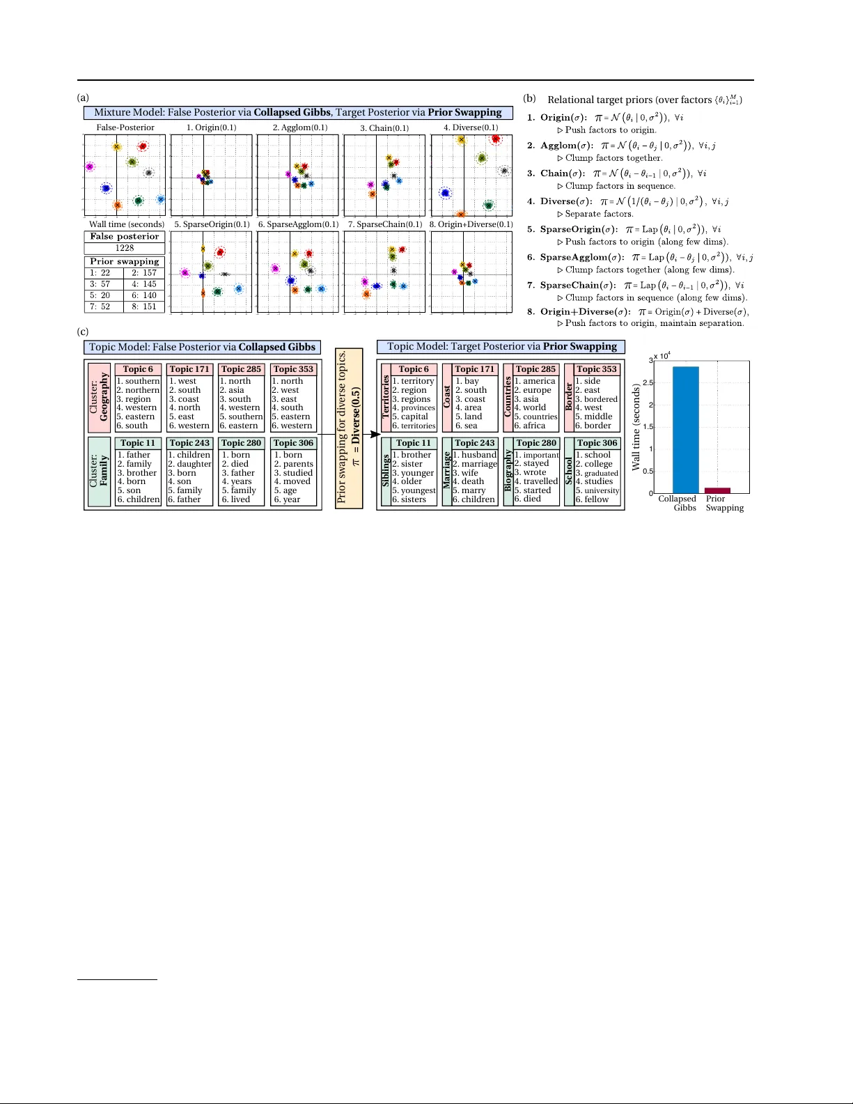
P ost-Infer ence Prior Swapping Willie Neiswanger 1 Eric Xing 2 Abstract While Bayesian methods are praised for their ability to incorporate useful prior knowledge, in practice, con v enient priors that allo w for compu- tationally cheap or tractable inference are com- monly used. In this paper , we in vestigate the fol- lowing question: for a given model, is it possible to compute an inference r esult with any conve- nient false prior , and afterwar ds, given any tar- get prior of interest, quickly tr ansform this re- sult into the tar get posterior? A potential solu- tion is to use importance sampling (IS). How- ev er, we demonstrate that IS will fail for many choices of the target prior , depending on its para- metric form and similarity to the f alse prior . In- stead, we propose prior sw apping, a method that lev erages the pre-inferred false posteri or to ef fi- ciently generate accurate posterior samples un- der arbitrary target priors. Prior swapping lets us apply less-costly inference algorithms to certain models, and incorporate ne w or updated prior in- formation “post-inference”. W e giv e theoretical guarantees about our method, and demonstrate it empirically on a number of models and priors. 1. Introduction There are many cases in Bayesian modeling where a cer- tain choice of prior distribution allo ws for computationally simple or tractable inference. For example, • Conjugate priors yield posteriors with a kno wn para- metric form and therefore allo w for non-iterati ve, ex- act inference ( Diaconis et al. , 1979 ). • Certain priors yield models with tractable conditional or mar ginal distrib utions, which allows efficient ap- proximate inference algorithms to be applied (e.g. Gibbs sampling ( Smith & Roberts , 1993 ), sampling 1 Carnegie Mellon Univ ersity , Machine Learning Department, Pittsbur gh, USA 2 CMU School of Computer Science. Correspon- dence to: W illie Neiswanger < willie@cs.cmu.edu > . Pr oceedings of the 34 th International Confer ence on Machine Learning , Sydne y , Australia, PMLR 70, 2017. Copyright 2017 by the author(s). in collapsed models ( T eh et al. , 2006 ), or mean-field variational methods ( W ang & Blei , 2013 )). • Simple parametric priors allo w for computationally cheap density queries, maximization, and sampling, which can reduce costs in iterativ e inference algo- rithms (e.g. Metropolis-Hastings ( Metropolis et al. , 1953 ), gradient-based MCMC ( Neal , 2011 ), or se- quential Monte Carlo ( Doucet et al. , 2000 )). For these reasons, one might hope to infer a result under a con venient-but-unrealistic prior , and afterwards, attempt to correct the result. More generally , gi ven an inference result (under a con venient prior or otherwise), one might wish to incorporate updated prior information, or see a result un- der different prior assumptions, without having to re-run a costly inference algorithm. This leads to the main question of this paper: for a giv en model, is it possible to use any con venient false prior to infer a false posterior , and afterwards, given any target prior of interest, efficiently and accurately infer the associated target posterior? One potential strategy in volv es sampling from the false posterior and reweighting these samples via importance sampling (IS). Ho wev er, depending on the chosen target prior—both its parametric form and similarity to the false prior—the resulting inference can be inaccurate due to high or infinite v ariance IS estimates (demonstrated in Sec. 2.1 ). W e instead aim to devise a method that yields accurate in- ferences for arbitrary target priors. Furthermore, lik e IS, we want to make use of the pre-inferred false posterior, without simply running standard inference algorithms on the target posterior . Note that most standard inference algorithms are iterativ e and data-dependent : parameter updates at each it- eration in volv e data, and the computational cost or quality of each update depends on the amount of data used. Hence, running inference algorithms directly on the target poste- rior can be costly (especially given a large amount of data or man y target priors of interest) and defeats the purpose of using a con venient false prior . In this paper , we propose prior swapping , an iterati ve, data- independent method for generating accurate posterior sam- ples under arbitrary target priors. Prior swapping uses the pre-inferred false posterior to perform efficient updates that Post-Infer ence Prior Swapping do not depend on the data, and thus proceeds very quickly . W e therefore advocate breaking dif ficult inference prob- lems into two easier steps: first, do inference using the most computationally con venient prior for a giv en model, and then, for all future priors of interest, use prior swapping. In the following sections, we demonstrate the pitfalls of using IS, describe the proposed prior swapping methods for different types of false posterior inference results (e.g. exact or approximate density functions, or samples) and giv e theoretical guarantees for these methods. Finally , we show empirical results on hea vy-tailed and sparsity priors in Bayesian generalized linear models, and relational priors ov er components in mixture and topic models. 2. Methodology Suppose we have a dataset of n v ectors x n = { x 1 , . . . , x n } , x i ∈ R p , and we hav e chosen a family of models with the likelihood function L ( θ | x n ) = p ( x n | θ ) , parameterized by θ ∈ R d . Suppose we hav e a prior distrib ution ov er the space of model parameters θ , with probability density func- tion (PDF) π ( θ ) . The likelihood and prior define a joint model with PDF p ( θ , x n ) = π ( θ ) L ( θ | x n ) . In Bayesian in- ference, we are interested in computing the posterior (con- ditional) distribution of this joint model, with PDF p ( θ | x n ) = π ( θ ) L ( θ | x n ) R π ( θ ) L ( θ | x n ) dθ . (1) Suppose we’ ve chosen a different prior distribution π f ( θ ) , which we refer to as a false prior (while we refer to π ( θ ) as the tar get prior ). W e can now define a ne w posterior p f ( θ | x n ) = π f ( θ ) L ( θ | x n ) R π f ( θ ) L ( θ ) | x n ) dθ (2) which we refer to as a false posterior . W e are interested in the follo wing task: giv en a f alse poste- rior inference result (i.e. samples from p f ( θ | x n ) , or some exact or approximate PDF), choose an arbitrary tar get prior π ( θ ) and ef ficiently sample from the associated target pos- terior p ( θ | x n ) —or , more generally , compute an expecta- tion µ h = E p [ h ( θ )] for some test function h ( θ ) with re- spect to the target posterior . 2.1. Importance Sampling and Prior Sensitivity W e begin by describing an initial strategy , and existing work in a related task kno wn as prior sensiti vity analysis. Suppose we hav e T false posterior samples { ˜ θ t } T t =1 ∼ p f ( θ | x n ) . In importance sampling (IS), samples from an importance distrib ution are used to estimate the expecta- tion of a test function with respect to a target distribution. A straightforward idea is to use the false posterior as an importance distribution, and compute the IS estimate ˆ µ IS h = T X t =1 w ( ˜ θ t ) h ( ˜ θ t ) (3) where the weight function w ( θ ) ∝ p ( θ | x n ) p f ( θ | x n ) ∝ π ( θ ) π f ( θ ) , and the T weights are normalized to sum to one. IS-based methods have been de veloped for the task of prior sensitivity analysis (PSA). In PSA, the goal is to determine how the posterior v aries o ver a sequence of priors (e.g. over a parameterized family of priors π ( θ ; γ i ) , i = 0 , 1 , . . . ). Existing work has proposed inferring a single posterior un- der prior π ( θ ; γ 0 ) , and then using IS methods to infer fur- ther posteriors in the sequence ( Besag et al. , 1995 ; Hast- ings , 1970 ; Bornn et al. , 2010 ). This strategy is ef fectiv e when subsequent priors are sim- ilar enough, but breaks do wn when two priors are suffi- ciently dissimilar, or are from ill-matched parametric fam- ilies, which we illustrate in an example belo w . Note that, in general for IS, as T → ∞ , ˆ µ IS h → µ h al- most surely . Ho we ver , IS estimates can still fail in practice if ˆ µ IS h has high or infinite variance. If so, the variance of the weights w ( ˜ θ t ) will be large (a problem often referred to as weight degeneracy), which can lead to inaccurate es- timates. In our case, the variance of ˆ µ IS h is only finite if E p f  h ( θ ) 2 π ( θ ) 2 π f ( θ ) 2  ∝ E p  h ( θ ) 2 π ( θ ) π f ( θ )  < ∞ . (4) For a broad class of h , this is satisfied if there e xists M ∈ R such that π ( θ ) π f ( θ ) < M , ∀ θ ( Ge weke , 1989 ). Given some pre- inferred p f ( θ | x n ) with f alse prior π f ( θ ) , the accurac y of IS thus depends on the target prior of interest. For e xample, if π ( θ ) has heavier tails than π f ( θ ) , the variance of ˆ µ IS h will be infinite for many h . Intuitiv ely , we expect the variance to be higher for π that are more dissimilar to π f . W e show a concrete example of this in Fig. 1 . Consider a normal model for data x n ∼ N ( θ , 1) , with a standard nor- mal false prior π f ( θ ) = N ( θ | 0 , 1) . This yields a closed- form f alse posterior (due to the conjug ate π f ), which is also normal. Suppose we’ d like to estimate the posterior e xpec- tation under a Laplace target prior , with mean 10 and vari- ance 1, for test function h ( θ ) = θ (i.e. an estimate of the target posterior mean). W e draw T false posterior samples { ˜ θ t } T t =1 ∼ p f ( θ | x n ) , compute weights w ( ˜ θ t ) and IS esti- mate ˆ µ IS h , and compare it with the true expectation µ h . W e see in Fig. 1 that | µ h − ˆ µ IS h | slo ws significantly as T increases, and maintains a high error ev en as T is made very lar ge. W e can analyze this issue theoretically . Sup- pose we want | µ h − ˆ µ IS h | < δ . Since we kno w p f ( θ | x n ) is normal, we can compute a lower bound on the num- ber of false posterior samples T that would be needed for Post-Infer ence Prior Swapping − 2 0 2 4 6 8 10 12 0 0.5 1 1.5 PDF False poster ior samples = Figure 1. Importance sampling with f alse posterior samples. As the number of samples T grows, the difference between the IS estimate ˆ µ IS h and the true value µ h decreases increasingly slowly . The difference remains lar ge ev en when T = 10 8 . See text for analysis. the expected estimate to be within δ of µ h . Namely , if p f ( θ | x n ) = N ( θ | m, s 2 ) , in order for | µ h − E p f [ ˆ µ IS h ] | < δ , we’ d need T ≥ exp  1 2 s 2 ( | µ h − m | − δ ) 2  . In the example in Fig. 1 , we hav e m = 1 , s 2 = 0 . 25 , and µ h = 7 . 9892 . Hence, for | µ h − E p f [ ˆ µ IS h ] | < 1 , we’ d need T > 10 31 samples (see appendix for full details of this analysis). Note that this bound actually has nothing to do with the parametric form of π ( θ ) —it is based solely on the normal false posterior , and its distance to the target poste- rior mean µ h . Howe ver , e ven if this distance was small, the importance estimate would still hav e infinite variance due to the Laplace tar get prior . Further , note that the sit- uation can significantly worsen in higher dimensions, or if the false posterior has a lo wer v ariance. 2.2. Prior Swapping W e’ d like a method that will work well even when f alse and tar get priors π f ( θ ) and π ( θ ) are significantly different, or are from different parametric families, with performance that does not worsen (in accuracy nor computational com- plexity) as the priors are made more dissimilar . Redoing inference for each new target posterior can be very costly , especially when the data size n is large, be- cause the per -iteration cost of most standard inference al- gorithms scales with n , and many iterations may be needed for accurate inference. This includes both MCMC and se- quential monte carlo (SMC) algorithms (i.e. repeated-IS- methods that infer a sequence of distributions). In SMC, the per-iteration cost still scales with n , and the variance estimates can still be infinite if subsequent distributions are ill-matched. Instead, we aim to leverage the inferred false posterior to more-efficiently compute any future target posterior . W e begin by defining a prior swap density p s ( θ ) . Suppose for now that a false posterior inference algorithm has returned a density function ˜ p f ( θ ) (we will give more details on ˜ p f later; assume for no w that it is either equal to p f ( θ | x n ) or approximates it). W e then define the prior swap density as p s ( θ ) ∝ ˜ p f ( θ ) π ( θ ) π f ( θ ) . (5) Note that if ˜ p f ( θ ) = p f ( θ | x n ) , then p s ( θ ) = p ( θ | x n ) . Howe ver , depending on ho w we represent ˜ p f ( θ ) , p s ( θ ) can hav e a much simpler analytic representation than p ( θ | x n ) , which is typically defined via a likelihood function (i.e. a function of the data) and causes inference algorithms to hav e costs that scale with the data size n . Specifically , we will only use lo w-complexity ˜ p f ( θ ) that can be e valuated in constant time with respect to the data size n . Our general strategy is to use p s ( θ ) as a surrogate for p ( θ | x n ) in standard MCMC or optimization procedures, to yield data-independent algorithms with constant cost per it- eration. Intuitiv ely , the likelihood information is captured by the false posterior—we make use of this instead of the likelihood function, which is costly to e v aluate. More concretely , at each iteration in standard inference al- gorithms, we must e v aluate a data-dependent function asso- ciated with the posterior density . For exam ple, we e v aluate a function proportional to p ( θ | x n ) in Metropolis-Hastings (MH) ( Metropolis et al. , 1953 ), and ∇ θ log p ( θ | x n ) in gradient-based MCMC methods (such as Lange vin dynam- ics (LD) ( Rossky et al. , 1978 ) and Hamiltonian Monte Carlo (HMC) ( Neal , 2011 )) and in optimization procedures that yield a MAP point estimate. In prior swapping, we in- stead ev aluate p s ( θ ) in MH, or ∇ θ log p s ( θ ) in LD, HMC, or gradient optimization to a MAP estimate (see appendix for algorithm pseudocode). Here, each iteration only re- quires ev aluating a fe w simple analytic expressions, and thus has O (1) complexity with respect to data size. W e demonstrate prior sw apping on our pre vious example (using a normal false prior and Laplace target prior) in Fig. 2 , where we have a closed-form (normal PDF) ˜ p f ( θ ) . T o do prior swapping, we run a Metropolis-Hastings algo- rithm on the target density p s ( θ ) . Note that drawing each Post-Infer ence Prior Swapping − 2 0 2 4 6 8 10 12 0 0.5 1 1.5 PDF Prior s wa pping s amples = Figure 2. Using prior swapping to compute estimate ˆ µ PS h by drawing samples { θ t } T t =1 ∼ p s ( θ ) . sample in this Markov chain does not in volv e the data x n , and can be done in constant time with respect to n (which we can see by viewing the w all time for dif ferent T ). In Fig. 2 , we draw T samples { θ t } T t =1 ∼ p s ( θ ) , compute a sample estimate ˆ µ PS h = 1 T P T t =1 θ t , and compare it with the true value µ h . W e see that ˆ µ PS h con verges to µ h after a relativ ely small number of samples T . 2.3. Prior Swapping with False P osterior Samples The pre vious method is only applicable if our false poste- rior inference result is a PDF ˜ p f ( θ ) (such as in closed-form inference or v ariational approximations). Here, we de velop prior sw apping methods for the setting where we only ha ve access to samples { ˜ θ t } T f t =1 ∼ p f ( θ | x n ) . W e propose the following procedure: 1. Use { ˜ θ t } T f t =1 to form an estimate ˜ p f ( θ ) ≈ p f ( θ | x n ) . 2. Sample from p s ( θ ) ∝ π ( θ ) ˜ p f ( θ ) π f ( θ ) with prior swapping, as before. Note that, in general, p s ( θ ) only approximates p ( θ | x n ) . As a final step, after sampling from p s ( θ ) , we can: 3. Apply a correction to samples from p s ( θ ) . W e will describe two methods for applying a correction to p s samples—one in volving importance sampling, and one in volving semiparametric density estimation. Additionally , we will discuss forms for ˜ p f ( θ ) , guarantees about these forms, and ho w to optimize the choice of ˜ p f ( θ ) . In particu- lar , we will ar gue why (in constrast to the initial IS strategy) these methods do not fail when p ( θ | x n ) and p f ( θ | x n ) are very dissimilar or ha ve ill-matching parametric forms. Prior swap importance sampling . Our first proposal for applying a correction to prior sw ap samples in volv es IS: af- ter estimating some ˜ p f ( θ ) , and sampling { θ t } T t =1 ∼ p s ( θ ) , we can treat { θ t } T t =1 as importance samples, and compute the IS estimate ˆ µ PSis h = T X t =1 w ( θ t ) h ( θ t ) (6) where the weight function is now w ( θ ) ∝ p ( θ | x n ) p s ( θ ) ∝ p f ( θ | x n ) ˜ p f ( θ ) (7) and the weights are normalized so that P T t =1 w ( θ t ) = 1 . The key difference between this and the previous IS strat- egy is the weight function. Recall that, pre viously , an accu- rate estimate depended on the similarity between π ( θ ) and π f ( θ ) ; both the distance to and parametric form of π ( θ ) could produce high or infinite variance estimates. This was an issue because we wanted the procedure to work well for any π ( θ ) . Now , howe ver , the performance depends on the similarity between ˜ p f ( θ ) and p f ( θ | x n ) —and by using the false posterior samples, we can estimate a ˜ p f ( θ ) that well approximates p f ( θ | x n ) . Additionally , we can prove that certain choices of ˜ p f ( θ ) guarantee a finite v ariance IS esti- mate. Note that the variance of ˆ µ PSis h is only finite if E p f  h ( θ ) 2 p f ( θ | x n ) 2 ˜ p f ( θ ) 2  ∝ E p  h ( θ ) 2 p f ( θ | x n ) ˜ p f ( θ )  < ∞ . T o bound this, it is suf ficient to show that there exists M ∈ R such that p f ( θ | x n ) ˜ p f ( θ ) < M for all θ (assuming a test function h ( θ ) with finite v ariance) ( Ge weke , 1989 ). T o satisfy this condition, we will propose a certain parametric family ˜ p α f ( θ ) . Note that, to maintain a prior swapping pro- cedure with O (1) cost, we want a ˜ p α f ( θ ) that can be ev alu- ated in constant time. In general, a ˜ p α f ( θ ) with fe wer terms will yield a faster procedure. W ith these in mind, we pro- pose the following f amily of densities. Definition. For a parameter α = ( α 1 , . . . , α k ) , α j ∈ R p , k > 0 , let density ˜ p α f ( θ ) satisfy ˜ p α f ( θ ) ∝ π f ( θ ) k Y j =1 p ( α j | θ ) n/k (8) where p ( α j | θ ) denotes the model conditional PDF . The number of terms in ˜ p α f ( θ ) (and cost to ev aluate) is determined by the parameter k . Note that this family is Post-Infer ence Prior Swapping inspired by the true form of the false posterior p f ( θ | x n ) . Howe ver , ˜ p α f ( θ ) has constant-time ev aluation, and we can estimate its parameter α using samples { ˜ θ t } T f t =1 ∼ p f ( θ | x n ) . Furthermore, we hav e the following guarantees. Theorem 2.1. F or any α = ( α 1 , . . . , α k ) ⊂ R p and k > 0 let ˜ p α f ( θ ) be defined as in Eq. ( 8 ). Then, ther e exists M > 0 such that p f ( θ | x n ) ˜ p α f ( θ ) < M , for all θ ∈ R d . Corollary 2.1.1. F or { θ t } T t =1 ∼ p α s ( θ ) ∝ ˜ p α f ( θ ) π ( θ ) π f ( θ ) , w ( θ t ) = p f ( θ t | x n ) ˜ p α f ( θ t )  P T r =1 p f ( θ r | x n ) ˜ p α f ( θ r )  − 1 , and test function that satisfies V ar p [ h ( θ )] < ∞ , the variance of IS estimate ˆ µ PSis h = P T t =1 h ( θ t ) w ( θ t ) is finite . Proofs for these theorems are giv en in the appendix. Note that we do not kno w the normalization constant for ˜ p α f ( θ ) . This is not an issue for its use in prior swapping, since we only need access to a function proportional to p α s ( θ ) ∝ ˜ p α f ( θ ) π ( θ ) π f ( θ ) − 1 in most MCMC algorithms. Howe ver , we still need to estimate α , which is an issue be- cause the unknown normalization constant is a function of α . Fortunately , we can use the method of score matching ( Hyv ¨ arinen , 2005 ) to estimate α given a density such as ˜ p α f ( θ ) with unknown normalization constant. Once we ha ve found an optimal parameter α ∗ , we draw samples from p α ∗ s ( θ ) ∝ ˜ p α ∗ f ( θ ) π ( θ ) π f ( θ ) − 1 , compute weights for these samples (Eq. ( 7 )), and compute the IS estimate ˆ µ PSis h . W e give pseudocode for the full prior swap importance sampling procedure in Alg. 1 . Algorithm 1: Prior Swap Importance Sampling Input: False posterior samples { ˜ θ t } T f t =1 ∼ p f ( θ | x n ) . Output: IS estimate ˆ µ PSis h . 1 Score matching: estimate α ∗ using { ˜ θ t } T f t =1 . 2 Prior swapping: sample { θ t } T t =1 ∼ p α ∗ s ( θ ) ∝ ˜ p α ∗ f ( θ ) π ( θ ) π f ( θ ) . 3 Importance sampling: compute ˆ µ PSis h = P T t =1 h ( θ t ) w ( θ t ) . Semiparametric prior swapping. In the pre vious method, we chose a parametric form for ˜ p α f ( θ ) ; in general, ev en the optimal α will yield an inexact approximation to p f ( θ | x n ) . Here, we aim to incorporate methods that return an increasingly exact estimate ˜ p f ( θ ) when given more false posterior samples { ˜ θ t } T f t =1 . One idea is to use a nonparametric kernel density estimate ˜ p np f ( θ ) and plug this into p np s ( θ ) ∝ ˜ p np f ( θ ) π ( θ ) π f ( θ ) − 1 . Howe ver , nonparametric density estimates can yield inac- curate density tails and fare badly in high dimensions. T o help mitigate these problems, we turn to a semiparamet- ric estimate, which begins with a parametric estimate, and adjusts it as samples are generated. In particular , we use a density estimate that can be vie wed as the product of a parametric density estimate and a nonparametric correc- tion function ( Hjort & Glad , 1995 ). This density estimate is consistent as the number of samples T f → ∞ . Instead of (or in addition to) correcting prior swap samples with importance sampling, we can correct them by updating the nonparametric correction function as we continue to gener- ate false posterior samples. Giv en T f samples { ˜ θ t } T f t =1 ∼ p f ( θ | x n ) , we write the semi- parametric false posterior estimate as ˜ p sp f ( θ ) = 1 T f T f X t =1 " 1 b d K k θ − e θ t k b ! ˜ p α f ( θ ) ˜ p α f ( ˜ θ t ) # , (9) where K denotes a probability density kernel, with band- width b , where b → 0 as T f → ∞ (see ( W asserman , 2006 ) for details on probability density k ernels and bandwidth se- lection). The semiparametric prior swap density is then p sp s ( θ ) ∝ ˜ p sp f ( θ ) π ( θ ) π f ( θ ) = 1 T f T f X t =1 K  k θ − ˜ θ t k b  ˜ p α f ( θ ) π ( θ ) ˜ p α f ( ˜ θ t ) π f ( θ ) b d ∝ [ p α s ( θ )]   1 T f T f X t =1 K  k θ − ˜ θ t k b  ˜ p α f ( ˜ θ t )   . (10) Hence, the prior swap density p sp s ( θ ) is proportional to the product of two densities: the parametric prior swap density p α s ( θ ) , and a correction density . T o estimate expectations with respect to p sp s ( θ ) , we can follow Alg. 1 as before, but replace the weight function in the final IS estimate with w ( θ ) ∝ p sp s ( θ ) p α s ( θ ) ∝ 1 T f T f X t =1 K  k θ − ˜ θ t k b  ˜ p α f ( ˜ θ t ) . (11) One advantage of this strategy is that computing the weights doesn’t require the data—it thus has constant cost with respect to data size n (though its cost does increase with the number of false posterior samples T f ). Addition- ally , as in importance sampling, we can pro ve that this pro- cedure yields an exact estimate of E [ h ( θ )] , asymptotically , as T f → ∞ (and we can provide an explicit bound on the rate at which p sp s ( θ ) con verges to p ( θ | x n ) ). W e do this by showing that p sp s ( θ ) is consistent for p ( θ | x n ) . Theorem 2.2. Given false posterior samples { ˜ θ t } T f t =1 ∼ p f ( θ | x n ) and b  T − 1 / (4+ d ) f , the estimator p sp s is consis- tent for p ( θ | x n ) , i.e. its mean-squared err or satisfies sup p ( θ | x n ) E  Z ( p sp s ( θ ) − p ( θ | x n )) 2 dθ  < c T 4 / (4+ d ) f for some c > 0 and 0 < b ≤ 1 . The proof for this theorem is giv en in the appendix. Post-Infer ence Prior Swapping 3. Empirical Results W e show empirical results on Bayesian generalized lin- ear models (including linear and logistic regression) with sparsity and heavy tailed priors, and on latent factor mod- els (including mixture models and topic models) with re- lational priors ov er factors (e.g. div ersity-encouraging, agglomerate-encouraging, etc.). W e aim to demonstrate empirically that prior swapping efficiently yields correct samples and, in some cases, allo ws us to apply certain infer- ence algorithms to more-complex models than was pre vi- ously possible. In the following experiments, we will refer to the following procedures: • T arget posterior inference: some standard inference algorithm (e.g. MCMC) run on p ( θ | x n ) . • False posterior inference: some standard inference algorithm run on p f ( θ | x n ) . • False posterior IS: IS using samples from p f ( θ | x n ) . • Prior swap exact: prior swapping with closed-form ˜ p f ( θ ) = p f ( θ | x n ) . • Prior swap parametric: prior swapping with para- metric ˜ p α f ( θ ) given by Eq. ( 8 ). • Prior swap IS: correcting samples from ˜ p α f ( θ ) with IS. • Prior swap semiparametric: correcting samples from ˜ p α f ( θ ) with the semiparametric estimate IS pro- cedure. T o assess performance, we choose a test function h ( θ ) , and compute the Euclidean distance between µ h = E p [ h ( θ )] and some estimate ˆ µ h returned by a procedure. W e denote this performance metric by posterior err or = k µ h − ˆ µ h k 2 . Since µ h is typically not av ailable analytically , we run a single chain of MCMC on the target posterior for one mil- lion steps, and use these samples as ground truth to com- pute µ h . For timing plots, to assess error of a method at a giv en time point, we collect samples drawn before this time point, remove the first quarter as burn in, and add the time it takes to compute any of the corrections. 3.1. Sparsity Inducing and Heavy T ailed Priors in Bayesian Generalized Linear Models Sparsity-encouraging regularizers have gained a high lev el of popularity o ver the past decade due to their ability to pro- duce models with greater interpretability and parsimony . For e xample, the L 1 norm has been used to induce sparsity with great ef fect ( Tibshirani , 1996 ), and has been shown to be equiv alent to a mean-zero independent Laplace prior ( T ibshirani , 1996 ; See ger , 2008 ). In a Bayesian setting, in- ference giv en a sparsity prior can be difficult, and often re- quires a computationally intensiv e method (such as MH or HMC) or posterior approximations (e.g. expectation prop- agation ( Minka , 2001 )) that make factorization or paramet- ric assumptions ( Seeger , 2008 ; Gerwinn et al. , 2010 ). W e propose a cheap yet accurate solution: first get an inference result with a more-tractable prior (such as a normal prior), and then use prior swapping to quickly con vert the result to the posterior giv en a sparsity prior . Our first set of experiments are on Bayesian linear re- gression models, which we can write as y i = X i θ + ,  ∼ N (0 , σ 2 ) , θ ∼ π , i = 1 ,..., n . For π , we compute results on Laplace, Student’ s t, and V erySparse (with PDF V erySparse ( σ ) = Q d i =1 1 2 σ exp {−| θ i | 0 . 4 /σ } ( Seeger , 2008 )) priors. Here, a normal π f is conjugate and allows for exact false posterior inference. Our sec- ond set of experiments are on Bayesian logistic regres- sion models, which we write as y i ∼ Bern ( p i ) , p i = logistic ( X i θ ) , θ ∼ π , i = 1 ,..., n . which we will pair with both hea vy tailed priors and a hierarchical tar get prior π = N (0 , α − 1 I ) , α ∼ Gamma ( γ , 1) . For these experi- ments, we also use a normal π f . Howe ver , this false prior is no longer conjugate, and so we use MCMC to sample from p f ( θ | x n ) . For linear regression, we use the Y earPredictionMSD data set * , ( n = 515345 , d = 90 ), in which regression is used to predict the year associated with a a song, and for logistic re- gression we use the MiniBooNE particle identification data set † , ( n = 130065 , d = 50 ), in which binary classification is used to distinguish particles. In Fig. 3 , we compare prior swapping and IS methods, in order to show that the prior swapping procedures yield ac- curate posterior estimates, and to compare their speeds of con vergence. W e plot posterior error vs. wall time for each method’ s estimate of the posterior mean E p [ h ( θ )] = E p [ θ ] for two sparsity target priors (Laplace and V erySparse), for both linear and logistic regression. In linear regression (only), since the normal conjugate π f allows us to compute a closed form p f ( θ | x n ) , we can run the prior swap exact method, where ˜ p f ( θ ) = p f ( θ | x n ) . Howe ver , we can also sample from p f ( θ | x n ) to compute ˜ p α ∗ f ( θ ) , and therefore compare methods such as prior swap par ametric and the two correction methods. In logistic regression, we do not hav e a closed form p f ( θ | x n ) ; here, we only compare the methods that mak e use of samples from p f ( θ | x n ) . In Fig. 3 , we see that the prior swapping methods (particularly prior swap IS) quickly con verge to nearly zero posterior error . Additionally , in linear re gression, we see that prior swap parametric, using ˜ p f ( θ ) = ˜ p α ∗ f ( θ ) , yields similar posterior error as prior swap exact, which uses ˜ p f ( θ ) = p ( θ | x n ) . * https://archive.ics.uci.edu/ml/datasets/ YearPredictionMSD † https://archive.ics.uci.edu/ml/datasets/ MiniBooNE+particle+identification Post-Infer ence Prior Swapping 0 100 200 300 400 500 600 700 800 0 0.2 0.4 0.6 0.8 1 1.2 1.4 1.6 1.8 0 100 200 300 400 500 0 0.2 0.4 0.6 0.8 1 1.2 1.4 1.6 1.8 0 100 200 300 400 500 0 0.05 0.1 0.15 0.2 0.25 0.3 0.35 0.4 0.45 0 50 100 150 200 250 0 0.05 0.1 0.15 0.2 0.25 0.3 0.35 0.4 0.45 False p osterior IS, Prio r swap exact, Prior swap parametric, Prior swap IS, Prior swap SP Posterio r erro r Posterio r erro r Posterio r erro r Posterio r erro r Wall time (s) Wall time (s) Wall time (s) Wall time (s) Bayesian Linear Regression Bayesian Logistic Regress ion Figure 3. Comparison of prior swapping and IS methods for Bayesian linear and logistic regression under Laplace and V erySparse target priors. The prior swapping methods (particularly prior swap e xact and prior swap IS) quickly con verge to lo w posterior errors. − 0.15 − 0.1 − 0.05 0 0.05 0 10 20 30 40 50 60 − 0.15 − 0.1 − 0.05 0 0.05 0 10 20 30 40 50 60 − 0.15 − 0.1 − 0.05 0 0.05 0 10 20 30 40 50 60 − 0.06 − 0.04 − 0.02 0 0.02 0.04 0.06 − 0.06 − 0.04 − 0.02 0 0.02 0.04 0.06 − 0.06 − 0.04 − 0.02 0 0.02 0.04 0.06 − 0.06 − 0.04 − 0.02 0 0.02 0.04 0.06 − 0.06 − 0.04 − 0.02 0 0.02 0.04 0.06 − 0.06 − 0.04 − 0.02 0 0.02 0.04 0.06 − 0.06 − 0.04 − 0.02 0 0.02 0.04 0.06 − 0.06 − 0.04 − 0.02 0 0.02 0.04 0.06 − 0.06 − 0.04 − 0.02 0 0.02 0.04 0.06 − 0.06 − 0.04 − 0.02 0 0.02 0.04 0.06 − 0.2 − 0.15 − 0.1 − 0.05 0 0.05 − 0.2 − 0.1 0 0.1 − 0.2 − 0.15 − 0.1 − 0.05 0 0.05 − 0.2 − 0.1 0 0.1 − 0.2 − 0.15 − 0.1 − 0.05 0 0.05 − 0.2 − 0.1 0 0.1 − 0.2 − 0.15 − 0.1 − 0.05 0 0.05 − 0.2 − 0.1 0 0.1 − 0.2 − 0.15 − 0.1 − 0.05 0 0.05 − 0.2 − 0.1 0 0.1 − 0.2 − 0.15 − 0.1 − 0.05 0 0.05 − 0.2 − 0.1 0 0.1 = Normal(0.1) = Student's t(0.1) = Laplace(0.1) = Laplace(0.01) = VerySparse(0.1) = VerySparse(0.01) PDF Dimensions 2 and 3 Dimensions 4 and 5 PDF PDF = Laplace(0.1) = Laplace(0.01 ) = Laplace(0.001) Dimension 1 − 0.06 − 0.04 − 0.02 0 0.02 0.04 0.06 − 0.06 − 0.04 − 0.02 0 0.02 0.04 0.06 (a) (b) (c) (d) False poster ior inference (exact) Target pos terior inference (MCMC ) False poster ior IS Prior s wa p (exact) Wall time (s) Posterio r erro r Wall time (s) Posterio r erro r 0 200 400 600 800 1000 0 0.1 0.2 0.3 0.4 0.5 0.6 0.7 0.8 0.9 1 0 200 400 600 800 1000 0 0.1 0.2 0.3 0.4 0.5 0.6 0.7 0.8 0.9 1 Appl ication: fast inference in B ayesian lin ear regre ssion Figure 4. Prior swapping for fast inference in Bayesian linear models with sparsity and heavy-tailed priors: (a-b) Conv ergence plots showing that prior swapping performs accurate inference faster than the comparison methods and is robust to changing π . (c) Inferred 1-d density marginals when prior sparsity is increased. (d) Prior swapping results for a v ariety of different sparsity priors. In Fig. 4 , we show how prior swapping can be used for fast inference in Bayesian linear models with sparsity or heavy-tailed priors. W e plot the time needed to first com- pute the false posterior (via exact inference) and then run prior swapping (via the MH procedure) on some target pos- terior , and compare this with the MH algorithm run directly on the tar get posterior . In (a) and (b) we sho w con ver gence plots and see that prior swapping performs faster inference (by a few orders of magnitude) than direct MH. In plot (b) we reduce the variance of the tar get prior; while this hurts the accurac y of f alse posterior IS, prior swapping still quickly con verges to zero error . In (c) we sho w 1-d density marginals as we increase the prior sparsity , and in (d) we show prior sw apping results for v arious sparsity priors. In the appendix, we also include results on logistic regres- sion with the hierarchical target prior , as well as results for synthetic data where we are able to compare timing and posterior error as we tune n and d . 3.2. Priors over F actors in Latent V ariable Models Many latent v ariable models in machine learning—such as mixture models, topic models, probabilistic matrix factor- ization, and others—in volv e a set of latent factors (e.g. components or topics). Often, we’ d like to use priors that encourage interesting behaviors among the factors. For example, we might want dissimilar factors through a div ersity-promoting prior ( Kwok & Adams , 2012 ; Xie et al. , 2016 ) or for the factors to sho w some sort of spar- sity pattern ( Mayrink et al. , 2013 ; Kno wles & Ghahramani , 2011 ). Inference in such models is often computationally expensi ve or designed on a case-by-case basis ( Xie et al. , 2016 ; Knowles & Ghahramani , 2011 ). Howe ver , when conjugate priors are placed over the factor parameters, collapsed Gibbs sampling can be applied. In this method, the factor parameters are integrated out, leav- ing only a subset of variables; on these, the conditional Post-Infer ence Prior Swapping (a) (b) Collapsed Gibb s Prior Swapping Wall time (seconds) 0 0.5 1 1.5 2 2.5 3 x 10 4 1. southern 2. northern 3. region 4. western 5. eastern 6. south Topic 6 Topic Model: False Pos terior via Co ll aps ed Gibbs Cluster: Geograph y Cluster: Fam ily 1. west 2. south 3. coast 4. north 5. east 6. western Topic 17 1 1. north 2. asia 3. south 4. western 5. southern 6. eastern Topic 28 5 1. father 2. family 3. brother 4. born 5. son 6. children Topic 11 1. children 2. daughter 3. born 4. son 5. family 6. father Topic 24 3 1. born 2. died 3. father 4. years 5. family 6. lived Topic 28 0 1. born 2. parents 3. studied 4. moved 5. age 6. year Topic 30 6 1. north 2. west 3. east 4. south 5. eastern 6. western Topic 35 3 Topic Model: Target P osterior via Prior Swappi ng 1. brother 2. sister 3. younger 4. older 5. youngest 6. sisters Topic 11 1. husband 2. marriage 3. wife 4. death 5. marry 6. children Topic 24 3 1. school 2. college 3. graduated 4. studies 5. university 6. fellow Topic 30 6 Topic 28 0 1. important 2. stayed 3. wrote 4. travelled 5. started 6. died 1. territo ry 2. region 3. regions 4. provinces 5. capital 6. territorie s Topic 6 Territo ries 1. bay 2. south 3. coast 4. area 5. land 6. sea Topic 17 1 Coast 1. america 2. europ e 3. asia 4. world 5. countries 6. africa Topic 28 5 Count ries 1. side 2. east 3. bordered 4. west 5. middle 6. border Topic 35 3 Bor der Sibli ngs Marriag e Biograph y School Prior s wa pping f or divers e topics. = Div erse(0.5) (c) Relational target prior s (over factors ) − 3 − 2 − 1 0 1 2 3 4 − 3 − 2 − 1 0 1 2 3 4 − 3 − 2 − 1 0 1 2 3 4 − 3 − 2 − 1 0 1 2 3 4 − 3 − 2 − 1 0 1 2 3 4 − 3 − 2 − 1 0 1 2 3 4 − 3 − 2 − 1 0 1 2 3 4 − 3 − 2 − 1 0 1 2 3 4 − 3 − 2 − 1 0 1 2 3 4 − 3 − 2 − 1 0 1 2 3 4 − 3 − 2 − 1 0 1 2 3 4 − 3 − 2 − 1 0 1 2 3 4 − 3 − 2 − 1 0 1 2 3 4 − 3 − 2 − 1 0 1 2 3 4 − 3 − 2 − 1 0 1 2 3 4 − 3 − 2 − 1 0 1 2 3 4 − 3 − 2 − 1 0 1 2 3 4 − 3 − 2 − 1 0 1 2 3 4 3. Chain(0.1) 7. SparseChain(0.1) 8. Origin+Diverse(0.1) 6. SparseAgglo m(0.1) False-Pos terior 1. Origin(0.1) 2. Agglom(0.1) 4. Diverse(0.1) 5. SparseOrigin(0.1) Wall time (seconds) Mixture Model: False Posterio r via Co ll aps ed Gibbs , Target Poster ior via Prior Swapping Figure 5. Latent factor models: (a) Prior swapping results for relational tar get priors (defined in (b)) o ver components in a mixture model. (c) Prior swapping with a div ersity-promoting target prior on an LD A topic model (Simple English W ikipedia corpus) to separate redundant topic clusters; the top 6 words per topic are sho wn. In (a, c) we show w all times for the initial inference and prior swapping. distributions can be computed analytically , which allows for Gibbs sampling over these variables. Afterwards, sam- ples of the collapsed factor parameters can be computed. Hence, we propose the following strategy: first, assign a prior for the factor parameters that allows for collapsed Gibbs sampling; afterwards, reconstruct the f actor samples and apply prior swapping for more complex relational pri- ors o ver the factors. W e can thus perform con venient infer- ence in the collapsed model, yet apply more-sophisticated priors to variables in the uncollapsed model. W e first show results on a Gaussian mixture model (GMM), written x i ∼ N ( µ z i , Σ z i ) , z i ∼ Dir ( α ) , { µ m } M m =1 ∼ π , i = 1 ,..., n . Using a normal π f ov er { µ m } M m =1 allows for collapsed Gibbs sampling. W e also show results on a topic model (latent Dirichlet allocation (LDA) ( Blei et al. , 2003 )) for te xt data (for the form of this model, see ( Blei et al. , 2003 ; W ang & Blei , 2011 )). Here, using a Dirichlet π f ov er topics allo ws for collapsed Gibbs sampling. For mixture models, we generate synthetic data from the abov e model ( n =10,000, d =2, M =9), and for topic models, we use the Simple English W ikipedia ‡ corpus (n=27,443 doc- uments, vocab=10,192 w ords), and set M =400 topics. ‡ https://simple.wikipedia.org/ In Fig. 5 , we show results for mixture and topic models. In (a) we show inferred posteriors over GMM components for a number of relational tar get priors, which we define in (b). In (c), we apply the di versity-promoting target prior to LD A, to separate redundant topics. Here, we show two topic clusters (“geography” and “family”) in p f ( θ | x n ) , which are separated into distinct, yet thematically-similar , topics after prior swapping. In (a) and (c) we also show wall times of the inference methods. 4. Conclusion Giv en some false posterior inference result, and an arbi- trary target prior, we have studied methods to accurately compute the associated target posterior (or expectations with respect to it), and to do this efficiently by le verag- ing the pre-inferred result. W e hav e argued and sho wn em- pirically that this strategy is ef fective e ven when the f alse and target posteriors are quite dissimilar . W e belie ve that this strategy shows promise to allow a wider range of (and possibly less-costly) inference alorithms to be applied to certain models, and to allo w updated or new prior infor - mation to be more-easily incorporated into models without re-incurring the full costs of standard inference algorithms. Post-Infer ence Prior Swapping 5. Acknowledgements W . Neiswanger and E. Xing are supported by NSF BigData Grant IIS1447676. References Besag, Julian, Green, Peter , Higdon, David, and Mengersen, Kerrie. Bayesian computation and stochas- tic systems. Statistical science , pp. 3–41, 1995. Blei, David M, Ng, Andrew Y , and Jordan, Michael I. La- tent dirichlet allocation. The J ournal of Machine Learn- ing Resear ch , 3:993–1022, 2003. Bornn, Luke, Doucet, Arnaud, and Gottardo, Raphael. An efficient computational approach for prior sensitiv- ity analysis and cross-validation. Canadian J ournal of Statistics , 38(1):47–64, 2010. Diaconis, Persi, Ylvisaker , Donald, et al. Conjugate priors for exponential families. The Annals of statistics , 7(2): 269–281, 1979. Doucet, Arnaud, Godsill, Simon, and Andrieu, Christophe. On sequential monte carlo sampling methods for bayesian filtering. Statistics and computing , 10(3):197– 208, 2000. Gerwinn, Sebastian, Macke, Jakob H, and Bethge, Matthias. Bayesian inference for generalized linear mod- els for spiking neurons. F r ontiers in Computational Neu- r oscience , 4(12), 2010. Gewek e, John. Bayesian inference in econometric models using monte carlo inte gration. Econometrica: Journal of the Econometric Society , pp. 1317–1339, 1989. Hastings, W Keith. Monte carlo sampling methods using markov chains and their applications. Biometrika , 57(1): 97–109, 1970. Hjort, Nils Lid and Glad, Ingrid K. Nonparametric density estimation with a parametric start. The Annals of Statis- tics , pp. 882–904, 1995. Hyv ¨ arinen, Aapo. Estimation of non-normalized statistical models by score matching. Journal of Machine Learning Resear ch , 6(Apr):695–709, 2005. Knowles, David and Ghahramani, Zoubin. Nonparametric bayesian sparse f actor models with application to gene expression modeling. The Annals of Applied Statistics , pp. 1534–1552, 2011. Kwok, James T and Adams, Ryan P . Priors for diversity in generativ e latent v ariable models. In Advances in Neur al Information Pr ocessing Systems , pp. 2996–3004, 2012. Mayrink, V inicius Diniz, Lucas, Joseph Edward, et al. Sparse latent factor models with interactions: Analysis of gene expression data. The Annals of Applied Statis- tics , 7(2):799–822, 2013. Metropolis, Nicholas, Rosenbluth, Arianna W , Rosenbluth, Marshall N, T eller , Augusta H, and T eller , Edward. Equation of state calculations by fast computing ma- chines. The journal of chemical physics , 21(6):1087– 1092, 1953. Minka, Thomas P . Expectation propagation for approx- imate bayesian inference. In Pr oceedings of the Sev- enteenth confer ence on Uncertainty in artificial intelli- gence , pp. 362–369. Morgan Kaufmann Publishers Inc., 2001. Neal, R. MCMC using hamiltonian dynamics. Handbook of Markov Chain Monte Carlo , pp. 113–162, 2011. Rossky , PJ, Doll, JD, and Friedman, HL. Bro wnian dy- namics as smart monte carlo simulation. The Journal of Chemical Physics , 69(10):4628–4633, 1978. Seeger , Matthias W . Bayesian inference and optimal de- sign for the sparse linear model. The J ournal of Mac hine Learning Resear ch , 9:759–813, 2008. Smith, Adrian FM and Roberts, Gareth O. Bayesian com- putation via the gibbs sampler and related markov chain monte carlo methods. Journal of the Royal Statistical Society . Series B (Methodological) , pp. 3–23, 1993. T eh, Y ee W , Ne wman, David, and W elling, Max. A col- lapsed variational bayesian inference algorithm for latent dirichlet allocation. In Advances in neur al information pr ocessing systems , pp. 1353–1360, 2006. T ibshirani, Robert. Regression shrinkage and selection via the lasso. J ournal of the Royal Statistical Society . Series B (Methodological) , pp. 267–288, 1996. W ang, Chong and Blei, Da vid M. Collaborativ e topic mod- eling for recommending scientific articles. In Pr oceed- ings of the 17th A CM SIGKDD international confer ence on Knowledge discovery and data mining , pp. 448–456. A CM, 2011. W ang, Chong and Blei, David M. V ariational inference in nonconjugate models. The J ournal of Mac hine Learning Resear ch , 14(1):1005–1031, 2013. W asserman, Larry . All of nonparametric statistics . Springer Science & Business Media, 2006. Xie, Pengtao, Zhu, Jun, and Xing, Eric. Div ersity- promoting bayesian learning of latent v ariable models. In Pr oceedings of the 33st International Confer ence on Machine Learning (ICML-16) , 2016. Post-Infer ence Prior Swapping A ppendix for “P ost-Inference Prior Swapping” A. Details on the IS Example (Sec. 2.1 ) Here we provide details on the IS e xample (for a normal π f and Laplace π ) giv en in Sec. 2.1 . W e made the following statement: if p f ( θ | x n ) = N ( θ | m, s 2 ) , in order for | µ h − E p f [ ˆ µ IS h ] | < δ , we need T ≥ exp  1 2 s 2 ( | µ h − m | − δ ) 2  . T o show this, we first gi ve an upper bound on the e xpected v alue of the maximum of T zero-mean s 2 -variance Gaussian random variables. Let { ˜ θ t } T t =1 ∼ g , where g ( θ ) = N ( θ | 0 , s 2 ) , and let Z = max t { ˜ θ t } T t =1 . Then, for some b > 0 , exp { b E g [ Z ] } ≤ E g [exp { bZ } ] = E g  max t n exp { b ˜ θ t } o T t =1  ≤ T X t =1 E g h exp { b ˜ θ t } i = T exp { b 2 s 2 / 2 } , where the first inequality is due to Jensen’ s inequality , and the final equality is due to the definition of a Gaussian moment generating function. The above implies that E g [ Z ] ≤ log T b + bs 2 2 . Setting b = q 2 s 2 log T , we hav e that E g h max t { ˜ θ t } T t =1 i = E g [ Z ] ≤ s p 2 log T . Howe ver , note that for all { ˜ θ t } T t =1 , and weights { w ( ˜ θ t ) } T t =1 (such that P T t =1 w ( ˜ θ t ) = 1 ), the IS estimate ˆ µ IS h for h ( θ ) = θ must be less than or equal to max t { ˜ θ t } T t =1 (since the weighted av erage of { ˜ θ t } T t =1 cannot be lar ger than the maximum of this set). Therefore, E g  ˆ µ IS h  ≤ E g h max t { ˜ θ t } T t =1 i ≤ s p 2 log T , and equiv alently T ≥ exp  1 2 s 2 E g  ˆ µ IS h  2  . In our example, we wanted the expected estimate to be within δ of µ h , i.e. we wanted | µ h − E g [ ˆ µ IS h ] | < δ ⇐ ⇒ δ − µ h ≤ E g [ ˆ µ IS h ] ≤ µ h + δ , and therefore, T ≥ exp  1 2 s 2 E g  ˆ µ IS h  2  ≥ exp  1 2 s 2 ( δ − µ h ) 2  . Finally , notice that the original statement in volv ed samples { ˜ θ t } T t =1 ∼ p f ( θ | x n ) = N ( m, s 2 ) (instead of from g = N (0 , s 2 ) ). But this is equi valent to setting p f ( θ | x n ) = g ( θ ) , and shifting our goal so that we w ant δ − | µ h − m | ≤ E p f [ ˆ µ IS h ] ≤ | µ h − m | + δ . This giv es us the desired bound: T ≥ exp  1 2 s 2 E p f  ˆ µ IS h  2  ≥ exp  1 2 s 2 ( δ − | µ h − m | ) 2  . Post-Infer ence Prior Swapping B. Prior Swapping Pseudocode (f or a false posterior PDF inference r esult ˜ p f ( θ ) ) Here we gi ve pseudocode for the prior swapping procedure, gi ven some false posterior PDF inference result ˜ p f ( θ ) , using the prior sw ap functions p s ( θ ) ∝ ˜ p f ( θ ) π ( θ ) π f ( θ ) and ∇ θ log p s ( θ ) ∝ ∇ θ log ˜ p f ( θ ) + ∇ θ log π ( θ ) − ∇ θ log π f ( θ ) , as described in Sec. 2.2 . In Alg. 2 , we show prior sw apping via the Metropolis-Hastings algorithm, which makes repeated use of p s ( θ ) . In Alg. 3 we show prior swapping via Hamiltonian Monte Carlo, which makes repeated use of ∇ θ log p s ( θ ) . A special case of Alg. 3 , which occurs when we set the number of simulation steps to L = 1 (in line 6), is prior swapping via Lange vin dynamics. Algorithm 2: Prior swapping via Metropolis-Hastings. Input: Prior swap function p s ( θ ) , and proposal q . Output: Samples { θ t } T t =1 ∼ p s ( θ ) as T → ∞ . 1 Initialize θ 0 .  Initialize Mark ov chain. 2 for t = 1 , . . . , T do 3 Draw θ s ∼ q ( θ s | θ t − 1 ) .  Propose ne w sample. 4 Draw u ∼ Unif ([0 , 1]) . 5 if u < min n 1 , p s ( θ s ) q ( θ t | θ s ) p s ( θ t ) q ( θ s | θ t ) o then 6 Set θ t ← θ s .  Accept proposed sample. 7 else 8 Set θ t ← θ t − 1 .  Reject proposed sample. Algorithm 3: Prior swapping via Hamiltonian Monte Carlo. Input: Prior swap function p s ( θ ) , its gradient-log ∇ θ log p s ( θ ) , and step-size  . Output: Samples { θ t } T t =1 ∼ p s ( θ ) as T → ∞ . 1 Initialize θ 0 .  Initialize Mark ov chain. 2 for t = 1 , . . . , T do 3 Draw r t ∼ N (0 , I ) . 4 Set ( e θ 0 , e r 0 ) ← ( θ t − 1 , r t − 1 ) 5 Set e r 0 ← e r 0 +  2 ∇ θ log p s ( e θ 0 ) .  Propose ne w sample (next 4 lines). 6 for l = 1 , . . . , L do 7 Set e θ l ← e θ l − 1 +  e r l − 1 . 8 Set e r l ← e r l − 1 +  ∇ θ log p s ( e θ l ) . 9 Set e r L ← e r L +  2 ∇ θ log p s ( e θ L ) . 10 Draw u ∼ Unif ([0 , 1]) . 11 if u < min n 1 , p s ( e θ L ) e r > L e r L p s ( θ t − 1 ) r > t − 1 r t − 1 o then 12 Set θ t ← b θ L .  Accept proposed sample. 13 else 14 Set θ t ← θ t − 1 .  Reject proposed sample. Post-Infer ence Prior Swapping C. Proofs of Theor etical Guarantees Here, we prov e the theorems stated in Sec. 2.3 . Throughout this analysis, we assume that we have T samples { ˜ θ t } T f t =1 ⊂ X ⊂ R d from the false-posterior p f ( θ | x n ) , and that b ∈ R + denotes the bandwidth of our semiparametric false-posterior density estimator ˜ p sp f ( θ ) . Let H ¨ older class Σ(2 , L ) on X be defined as the set of all  = b 2 c times dif ferentiable functions f : X → R whose deriv ativ e f ( l ) satisfies | f ( ` ) ( θ ) − f ( ` ) ( θ 0 ) | ≤ L | θ − θ 0 | 2 − ` for all θ , θ 0 ∈ X . Let the class of densities P (2 , L ) be P (2 , L ) =  f ∈ Σ(2 , L )    f ≥ 0 , Z f ( θ ) dθ = 1  . Let data x n = { x 1 , . . . , x n } ⊂ Y ⊂ R p , let Z ⊂ Y be any set such that x n ⊂ Z , and let F Z ( L ) denote the set of densities p : Y → R that satisfy | log p ( x ) − log p ( x 0 ) | ≤ L | x − x 0 | , for all x, x 0 ∈ Z . In the following theorems, we assume that the false-posterior density p f ( θ | x n ) is bounded, i.e. that there exists some B > 0 such that p f ( θ | x n ) ≤ B for all θ ∈ R d ; that the prior swap density p s ( θ ) ∈ P (2 , L ) ; and that the model family p ( x n | θ ) ∈ F Z ( L ) for some Z . Theorem 2.1. F or any α = ( α 1 , . . . , α k ) ⊂ R p and k > 0 let ˜ p α f ( θ ) be defined as in Eq. ( 8 ). Then, ther e exists M > 0 such that p f ( θ | x n ) ˜ p α f ( θ ) < M , for all θ ∈ R d . Pr oof. T o prove that there e xists M > 0 such that p f ( θ | x n ) ˜ p α f ( θ ) < M , note that the false posterior can be written p f ( θ | x n ) = 1 Z 1 π f ( θ ) n Y i =1 L ( θ | x i ) = 1 Z 1 π f ( θ ) n Y i =1 p ( x i | θ ) , and the parametric estimate ˜ p α f ( θ ) is defined to be ˜ p α f ( θ ) = 1 Z 2 π f ( θ ) k Y j =1 p ( α j | θ ) n/k . Let d = max i,j | x i − α j | . For any i ∈ { 1 , . . . , n } , j ∈ { 1 , . . . , k } , | log p ( x i | θ ) − log p ( α j | θ ) | ≤ Ld = ⇒     log p ( x i | θ ) p ( α j | θ )     ≤ Ld, and exp  log p ( x i | θ ) p ( α j | θ )  ≤ exp      log p ( x i | θ ) p ( α j | θ )      ≤ exp { Ld } = ⇒ p ( x i | θ ) p ( α j | θ ) ≤ exp { Ld } . Therefore p f ( θ | x n ) ˜ p α f ( θ ) ≤ Z 2 Z 1 Q n i =1 p ( x i | θ ) Q k j =1 p ( α j | θ ) n/k ≤ Z 2 Z 1 exp { nLd } = M . Post-Infer ence Prior Swapping Corollary 2.1.1. F or { θ t } T t =1 ∼ p α s ( θ ) ∝ ˜ p α f ( θ ) π ( θ ) π f ( θ ) , w ( θ t ) = p f ( θ t | x n ) ˜ p α f ( θ t )  P T r =1 p f ( θ r | x n ) ˜ p α f ( θ r )  − 1 , and test function that satisfies V ar p [ h ( θ )] < ∞ , the variance of IS estimate ˆ µ PSis h = P T t =1 h ( θ t ) w ( θ t ) is finite. Pr oof. This follo ws directly from the sufficient conditions for finite variance IS estimates gi ven by ( Ge weke , 1989 ), which we hav e prov ed are satisfied for ˆ µ PSis h in Theorem 2.1. Theorem 2.2. Given false posterior samples { ˜ θ t } T f t =1 ∼ p f ( θ | x n ) and b  T − 1 / (4+ d ) f , the estimator p sp s is consistent for p ( θ | x n ) , i.e. its mean-squared err or satisfies sup p ( θ | x n ) ∈P (2 ,L ) E  Z ( p sp s ( θ ) − p ( θ | x n )) 2 dθ  < c T 4 / (4+ d ) f for some c > 0 and 0 < b ≤ 1 . Pr oof. T o prov e mean-square consistency of our semiparametric prior swap density estimator p sp s , we giv e a bound on the mean-squared error (MSE), and show that it tends to zero as we increase the number of samples T f drawn from the false-posterior . T o prove this, we bound the bias and variance of the estimator , and use this to bound the MSE. In the following, to a void cluttering notation, we will drop the subscript p f in E p f [ · ] . W e first bound the bias of our semiparametric prior swap estimator . For any p ( θ | x n ) ∈ P (2 , L ) , we can write the bias as | E [ p sp s ( θ )] − p ( θ | x n ) | = c 1     E  ˜ p sp f ( θ ) π ( θ ) π f ( θ )  − p f ( θ | x n ) π ( θ ) π f ( θ )     = c 2     π ( θ ) π f ( θ ) E h ˜ p sp f ( θ ) i − p f ( θ | x n )     = c 3    E h ˜ p sp f ( θ ) i − p f ( θ | x n )    ≤ ch 2 for some c > 0 , where we ha ve used the fact that    E h ˜ p sp f ( θ ) i − p f ( θ | x n )    ≤ ˜ ch 2 for some ˜ c > 0 (gi ven in ( Hjort & Glad , 1995 ; W asserman , 2006 )). W e ne xt bound the v ariance of our semiparametric prior swap estimator . For any p ( θ | x n ) ∈ P (2 , L ) , we can write the variance of our estimator as V ar [ p sp s ( θ )] = c 1 V ar  ˜ p sp f ( θ ) π ( θ ) π f ( θ )  = π ( θ ) 2 π f ( θ ) 2 V ar h ˜ p sp f ( θ ) i ≤ c T f h d for some c > 0 , where we have used the facts that V ar h ˜ p sp f ( θ ) i ≤ c T h d for some c > 0 and E h ˜ p sp f ( θ ) i 2 ≤ ˜ c for some ˜ c > 0 (gi ven in ( Hjort & Glad , 1995 ; W asserman , 2006 )). Next, we will use these two results to bound the mean-squared error of our semiparametric prior swap estimator , which shows that it is mean-square consistent. W e can write the mean-squared error as the sum of the variance and the bias-squared, and therefore, E  Z ( p sp s ( θ ) − p ( θ | x n )) 2 dθ  ≤ c 1 h 2 + c 2 T h d = c T 4 / (4+ d ) f for some c > 0 , using the fact that h  T − 1 / (4+ d ) f . Post-Infer ence Prior Swapping D. Further Empirical Results Here we show further empirical results on a logistic regression model with hierarchical target prior giv en by π = N (0 , α − 1 I ) , α ∼ Gamma ( γ , 1) . W e use synthetic data so that we are able to compare the timing and posterior error of different methods as we tune n and d . In this experiment, we assume that we are giv en samples from a false posterior p f ( θ | x n ) , and we want to most- efficiently compute the tar get posterior under prior π ( θ ) . In addition to the prior swapping methods, we can run standard iterativ e inference algorithms, such as MCMC or variational inference (VI), on the target posterior (initializing them, for example, at the false posterior mode) as comparisons. The following experiments aim to show that, once the data size n grows large enough, prior swapping methods become more efficient than standard inference algorithms. They also aim to show that the held-out test error of prior swapping matches that of these standard inference algorithms. In these experiments, we also add a prior swap method called prior swapping VI ; this method inv olves making a VI approximation to p f ( θ | x n ) , and using it for ˜ p f ( θ ) . Prior swapping VI allo ws us to see whether the test error is similar to standard VI inference algorithms, which compute some approximation to the posterior . Finally , we sho w results over a range of target prior hyperparameter values γ to show that prior swapping maintains accuracy (i.e. has a similar error as standard inference algorithms) over the full range. W e show results in Fig. 6 . In (a) and (b) we vary the number of observations ( n =10-120,000) and see that prior swapping has a constant w all time while the wall times of both MCMC and VI increase with n . In (b) we see that the prior swapping methods achiev e the same test error as the standard inference methods. In (c) and (d) we v ary the number of dimensions ( d =1-40). In this case, all methods have increasing wall time, and again the test errors match. In (e), (f), and (g), we vary the prior hyperparameter ( γ =1-1.05). For prior swapping, we infer a single ˜ p f ( θ ) (using γ = 1 . 025 ) with both MCMC and VI applied to p f ( θ | x n ) , and compute all other hyperparameter results using this ˜ p f ( θ ) . This demonstrates that prior swapping can quickly infer correct results over a range of hyperparameters. Here, the prior swapping semiparametric method matches the test error of MCMC slightly better than the parametric method. Log wall time (log(seconds)) Test Erro r Test Erro r Total wall tim e (seco nds) Test Erro r Number of observations x10 4 Number of observations x10 4 Number of dimensions Number of dimensions 1. MC MC 2. VI 3. PS VI 4. PS Semi 5. PS Para Log wall time (log(seconds)) Log wall time (log(seconds)) 1 3,4,5 2 1 3,4,5 2 1 2,3,4,5 2,3 1,4,5 2,3 1,4,5 2,3 1,4,5 (a) (b) (c) (d) Hy perparameter Hy perparameter (e) (f) (g) 1 1.01 1.02 1.03 1.04 1.05 0.09 0.1 0.11 0.12 0.13 0.14 0.15 0.16 0.17 1 1.01 1.02 1.03 1.04 1.05 6 7 8 9 10 11 0 2 4 6 8 10 x 10 5 0 5 10 15 20 25 30 35 0.05 0.1 0.15 0.2 0.25 0.3 0 5 10 15 20 25 30 35 3 4 5 6 7 8 9 10 11 0 2 4 6 8 10 x 10 4 0.09 0.1 0.11 0.12 0.13 0.14 0.15 0.16 0 2 4 6 8 10 x 10 4 2 4 6 8 10 12 1. Target po sterior inf . (MC MC ) 2. Target po sterior inf . (VI) 3. Prior swap VI 4. Prior swap semiparametric 5. Prior swap parametric Figure 6. Bayesian hierarchical logistic regression: (a-b) W all time and test error comparisons for varying data size n . As n is increased, w all time remains constant for prior swapping but grows for standard inference methods. (c-d) W all time and test error comparisons for varying model dimensionality d . (e-g) W all time and test error comparisons for inferences on a set of prior hyperparameters γ ∈ [1 , 1 . 05] . Here, a single false posterior ˜ p f ( θ ) (computed at γ = 1 . 025 ) is used for prior swapping on all other hyperparameters.