Toward Deeper Understanding of Neural Networks: The Power of Initialization and a Dual View on Expressivity

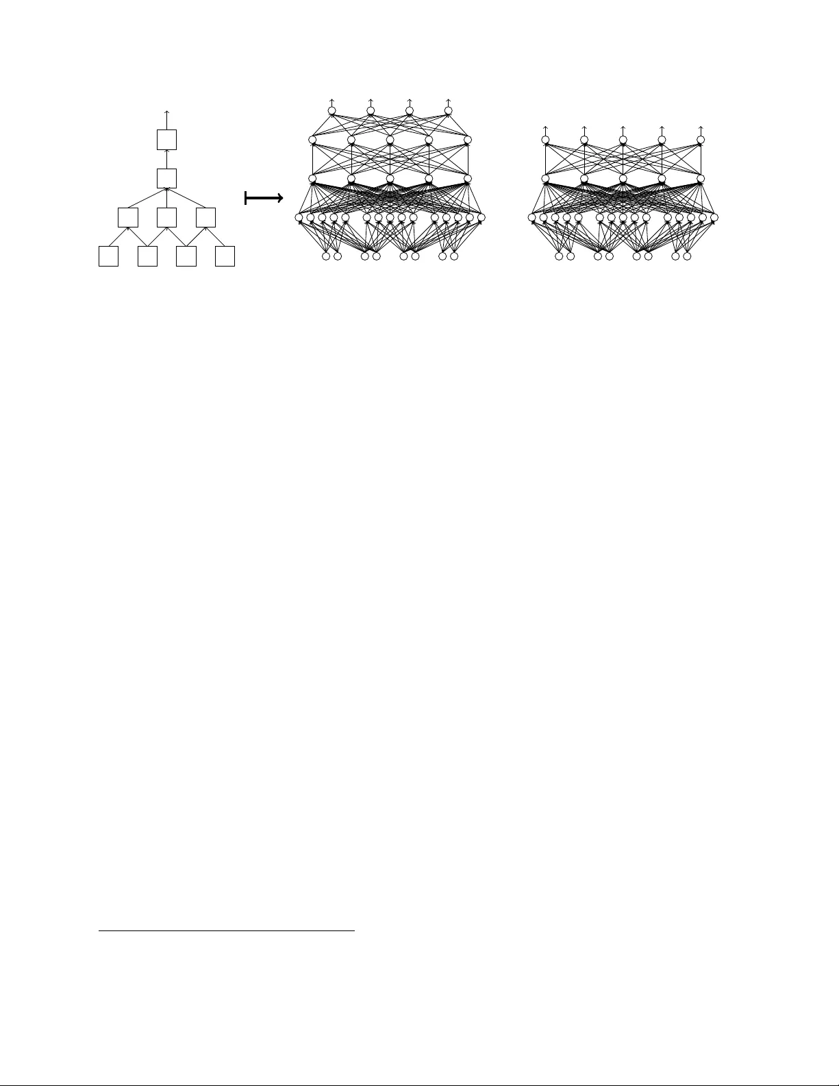
T o w ard Deep er Understanding of Neural Net w orks: The P o w er of Initialization and a Dual View on Expressivit y Amit Daniely ∗ Ro y F rostig † Y oram Singer ‡ Ma y 23, 2017 Abstract W e dev elop a general dualit y b et ween neural netw orks and comp ositional kernels, striving tow ards a better understanding of deep learning. W e sho w that initial repre- sen tations generated by common random initializations are suﬃciently rich to express all functions in the dual kernel space. Hence, though the training ob jective is hard to optimize in the worst case, the initial weigh ts form a goo d starting p oint for opti- mization. Our dual view also reveals a pragmatic and aesthetic p ersp ective of neural net works and underscores their expressive p o wer. ∗ Email: amitdaniely@go ogle.com † Email: rf@cs.stanford.edu. W ork performed at Go ogle. ‡ Email: singer@go ogle.com Con ten ts 1 In tro duction 1 2 Related w ork 2 3 Setting 3 4 Computation sk eletons 4 4.1 F rom computation sk eletons to neural net works . . . . . . . . 6 4.2 F rom computation sk eletons to repro ducing k ernels . . . . . . 7 5 Main results 9 5.1 Incorp orating bias terms . . . . . . . . . . . . . . . . . . . . . 11 6 Mathematical bac kground 11 7 Comp ositional k ernel spaces 13 8 The dual activ ation function 15 9 Pro ofs 20 9.1 W ell-behav ed activ ations . . . . . . . . . . . . . . . . . . . . . 20 9.2 Pro ofs of Thms. 2 and 3 . . . . . . . . . . . . . . . . . . . . . 23 9.3 Pro ofs of Thms. 4 and 5 . . . . . . . . . . . . . . . . . . . . . 26 10 Discussion 29 1 In tro duction Neural netw ork (NN) learning has underpinned state of the art empirical results in numer- ous applied machine learning tasks (see for instance [ 31 , 33 ]). Nonetheless, neural net work learning remains rather p o orly understo o d in sev eral regards. Notably , it remains unclear wh y training algorithms ﬁnd goo d weigh ts, how learning is impacted b y the net work arc hi- tecture and activ ations, what is the role of random w eight initialization, and ho w to choose a concrete optimization pro cedure for a giv en arc hitecture. W e start b y analyzing the expressiv e p ow er of NNs subsequent to the random w eigh t ini- tialization. The motiv ation is the empirical success of training algorithms despite inherent computational in tractabilit y , and the fact that they optimize highly non-con vex ob jectiv es with potentially many lo cal minima. Our k ey result shows that random initialization al- ready p ositions learning algorithms at a go o d starting p oint. W e deﬁne an ob ject termed a c omputation skeleton that describ es a distilled structure of feed-forw ard netw orks. A skele- ton induces a family of netw ork arc hitectures along with a h yp othesis class H of functions obtained by certain non-linear comp ositions according to the skeleton’s structure. W e sho w that the representation generated by random initialization is suﬃcien tly rich to approxi- mately express the functions in H . Concretely , all functions in H can b e approximated by tuning the weigh ts of the last lay er, whic h is a conv ex optimization task. In addition to explaining in part the success in ﬁnding go o d weigh ts, our study pro vides an app ealing p ersp ective on neural net w ork learning. W e establish a tigh t connection b e- t ween net work arc hitectures and their dual k ernel spaces. This connection generalizes sev eral previous constructions (see Sec 2 ). As we demonstrate, our dual view gives rise to design principles for NNs, supp orting curren t practice and suggesting new ideas. W e outline b elow a few p oin ts. • Duals of con volutional net w orks app ear a more suitable ﬁt for vision and acoustic tasks than those of fully connected net w orks. • Our framew ork surfaces a principled initialization sc heme. It is v ery similar to common practice, but incorp orates a small correction. • By mo difying the activ ation functions, t w o consecutive fully connected la yers can be replaced with one while preserving the net work’s dual kernel. • The ReLU activ ation, i.e. x 7→ max( x, 0), p ossesses fav orable prop erties. Its dual k ernel is expressive, and it can be w ell approximated by random initialization, ev en when the initialization’s scale is mo derately c hanged. • As the n um b er of la yers in a fully connected net work becomes v ery large, its dual k ernel con verges to a degenerate form for any non-linear activ ation. • Our result suggests that optimizing the weigh ts of the last lay er can serv e as a con- v ex pro xy for c ho osing among diﬀerent arc hitectures prior to training. This idea was adv o cated and tested empirically in [ 49 ]. 1 2 Related w ork Curren t theoretical understanding of NN learning. Understanding neural netw ork learning, particularly its recent successes, commonly decomp oses into the follo wing research questions. (i) W hat functions can b e eﬃciently expressed b y neural netw orks? (ii) When do es a low empirical loss result in a low p opulation loss? (iii) Wh y and when do eﬃcient algorithms, suc h as sto c hastic gradient, ﬁnd go o d weigh ts? Though still far from b eing complete, previous w ork pro vides some understanding of ques- tions (i) and (ii) . Standard results from complexit y theory [ 28 ] imply that essen tially all functions of in terest (that is, an y eﬃciently computable function) can b e expressed b y a net work of mo derate size. Biological phenomena show that man y relev ant functions can b e expressed b y ev en simpler net w orks, similar to conv olutional neural netw orks [ 32 ] that are dominan t in ML tasks to day . Barron’s theorem [ 7 ] states that ev en tw o-la yer net works can express a v ery rich set of functions. As for question (ii) , b oth classical [ 10 , 9 , 3 ] and more recen t [ 40 , 22 ] results from statistical learning theory show that as the num b er of examples gro ws in comparison to the size of the net w ork the empirical loss m ust b e close to the p op- ulation loss. In contrast to the ﬁrst t w o, question (iii) is rather p o orly understo o d. While learning algorithms succeed in practice, theoretical analysis is o verly p essimistic. Direct in terpretation of theoretical results suggests that when going sligh tly deep er beyond single la yer net works, e.g. to depth t wo netw orks with very few hidden units, it is hard to predict ev en marginally b etter than random [ 29 , 30 , 17 , 18 , 16 ]. Finally , w e note that the recent empirical successes of NNs hav e prompted a surge of theoretical work around NN learning [ 47 , 1 , 4 , 12 , 39 , 35 , 19 , 52 , 14 ]. Comp ositional k ernels and connections to netw orks. The idea of comp osing kernels has rep eatedly app eared throughout the mac hine learning literature, for instance in early w ork b y Sc h¨ olk opf et al. [ 51 ], Grauman and Darrell [ 21 ]. Inspired by deep netw orks’ s uccess, researc hers considered deep comp osition of kernels [ 36 , 13 , 11 ]. F or fully connected t w o-la yer net works, the corresp ondence b et ween k ernels and neural netw orks with random weigh ts has b een examined in [ 46 , 45 , 38 , 56 ]. Notably , Rahimi and Rech t [ 46 ] prov ed a formal connec- tion (similar to ours) for the RBF kernel. Their work w as extended to include p olynomial k ernels [ 27 , 42 ] as well as other kernels [ 6 , 5 ]. Sev eral authors ha ve further explored w a ys to extend this line of researc h to deep er, either fully-connected net works [ 13 ] or conv olutional net works [ 24 , 2 , 36 ]. Our work sets a common foundation for and expands on these ideas. W e extend the analysis from fully-connected and conv olutional net works to a rather broad family of arc hitectures. In addition, we prov e appro ximation guarantees b etw een a net work and its corresp onding kernel in our more general setting. W e th us extend previous analyses that only applies to fully connected tw o-lay er netw orks. Finally , we use the connection as an analytical to ol to reason ab out architectural design c hoices. 2 3 Setting Notation. W e denote v ectors b y b old-face letters (e.g. x ), and matrices b y upp er case Greek letters (e.g. Σ). The 2-norm of x ∈ R d is denoted by k x k . F or functions σ : R → R w e let k σ k := p E X ∼N (0 , 1) σ 2 ( X ) = q 1 √ 2 π R ∞ −∞ σ 2 ( x ) e − x 2 2 dx . Let G = ( V , E ) be a directed acyclic graph. The set of neigh b ors incoming to a v ertex v is denoted in( v ) := { u ∈ V | uv ∈ E } . The d − 1 dimensional sphere is denoted S d − 1 = { x ∈ R d | k x k = 1 } . W e pro vide a brief o v erview of reproducing k ernel Hilb ert spaces in the sequel and merely introduce notation here. In a Hilb ert space H , we use a sligh tly non-standard notation H B for the ball of radius B , { x ∈ H | k x k H ≤ B } . W e use [ x ] + to denote max( x, 0) and 1 [ b ] to denote the indicator function of a binary v ariable b . Input space. Throughout the pap er w e assume that eac h example is a sequence of n elemen ts, eac h of which is represented as a unit vector. Namely , we ﬁx n and take the input space to b e X = X n,d =  S d − 1  n . Eac h input example is denoted, x = ( x 1 , . . . , x n ) , where x i ∈ S d − 1 . (1) W e refer to eac h v ector x i as the input’s i th c o or dinate , and use x i j to denote it j th scalar en try . Though this notation is sligh tly non-standard, it uniﬁes input t yp es seen in v arious domains. F or example, binary features can be enco ded b y taking d = 1, in whic h case X = {± 1 } n . Mean while, images and audio signals are often represen ted as bounded and con tinuous n umerical v alues—w e can assume in full generalit y that these v alues lie in [ − 1 , 1]. T o matc h the setup ab ov e, we em b ed [ − 1 , 1] in to the circle S 1 , e.g. via the map x 7→  sin  π x 2  , cos  π x 2  . When eac h co ordinate is categorical—taking one of d v alues—we can represen t category j ∈ [ d ] b y the unit vector e j ∈ S d − 1 . When d may b e v ery large or the basic units exhibits some structure, suc h as when the input is a sequence of w ords, a more concise enco ding ma y be useful, e.g. as unit v ectors in a lo w dimension space S d 0 where d 0  d (see for instance Mikolo v et al. [ 37 ], Levy and Goldb erg [ 34 ]). Sup ervised learning. The goal in sup ervised learning is to devise a mapping from the input space X to an output space Y based on a sample S = { ( x 1 , y 1 ) , . . . , ( x m , y m ) } , where ( x i , y i ) ∈ X × Y , dra wn i.i.d. from a distribution D o v er X × Y . A sup ervised learning problem is further sp eciﬁed by an output length k and a loss function ` : R k × Y → [0 , ∞ ), and the goal is to ﬁnd a predictor h : X → R k whose loss, L D ( h ) := E ( x ,y ) ∼D ` ( h ( x ) , y ), is small. The empiric al loss L S ( h ) := 1 m P m i =1 ` ( h ( x i ) , y i ) is commonly used as a proxy for the loss L D . Regression problems corresp ond to Y = R and, for instance, the squared loss ` ( ˆ y , y ) = ( ˆ y − y ) 2 . Binary classiﬁcation is captured by Y = {± 1 } and, sa y , the zero-one loss ` ( ˆ y , y ) = 1 [ ˆ y y ≤ 0] or the hinge loss ` ( ˆ y , y ) = [1 − ˆ y y ] + , with standard extensions to the m ulticlass case. A loss ` is L -Lipsc hitz if | ` ( y 1 , y ) − ` ( y 2 , y ) | ≤ L | y 1 − y 2 | for all y 1 , y 2 ∈ R k , y ∈ Y , and it is conv ex if ` ( · , y ) is con vex for ev ery y ∈ Y . 3 Neural netw ork learning. W e deﬁne a neur al network N to b e a v ertices w eigh ted directed acyclic graph (D AG) whose no des are denoted V ( N ) and edges E ( N ). The weigh t function will b e denoted by δ : V ( N ) → [0 , ∞ ), and its sole role would b e to dictate the distribution of the initial weigh ts (see deﬁnition 3 ). Each of its in ternal units, i.e. no des with b oth incoming and outgoing edges, is asso ciated with an activation function σ v : R → R . In this pap er’s context, an activ ation can b e any function that is square in tegrable with resp ect to the Gaussian measure on R . W e say that σ is normalize d if k σ k = 1. The set of no des having only incoming edges are called the output no des. T o matc h the setup of a sup ervised learning problem, a net w ork N has nd input no des and k output no des, denoted o 1 , . . . , o k . A net work N together with a w eight v ector w = { w uv | uv ∈ E } deﬁnes a predictor h N , w : X → R k whose prediction is giv en by “propagating” x forward through the netw ork. F ormally , w e deﬁne h v , w ( · ) to be the output of the subgraph of the node v as follo ws: for an input no de v , h v , w outputs the corresp onding co ordinate in x , and for all other no des, w e deﬁne h v , w recursiv ely as h v , w ( x ) = σ v  P u ∈ in( v ) w uv h u, w ( x )  . Finally , w e let h N , w ( x ) = ( h o 1 , w ( x ) , . . . , h o k , w ( x )). W e also refer to internal no des as hidden units . The output layer of N is the sub-netw ork consisting of all output neurons of N along with their incoming edges. The r epr esentation induced b y a netw ork N is the netw ork rep( N ) obtained from N b y remo ving the output la yer. The r epr esentation function induced b y the w eigh ts w is R N , w := h rep( N ) , w . Giv en a sample S , a learning algorithm searches for w eights w having small empirical loss L S ( w ) = 1 m P m i =1 ` ( h N , w ( x i ) , y i ). A p opular approac h is to randomly initialize the w eights and then use a v ariant of the stochastic gradien t metho d to impro ve these w eigh ts in the direction of low er empirical loss. Kernel learning. A function κ : X × X → R is a r epr o ducing kernel , or simply a kernel, if for every x 1 , . . . , x r ∈ X , the r × r matrix Γ i,j = { κ ( x i , x j ) } is p ositive semi-deﬁnite. Eac h kernel induces a Hilb ert space H κ of functions from X to R with a corresp onding norm k · k H κ . A kernel and its corresp onding space are normalize d if ∀ x ∈ X , κ ( x , x ) = 1. Given a con v ex loss function ` , a sample S , and a kernel κ , a k ernel learning algorithm ﬁnds a function f = ( f 1 , . . . , f k ) ∈ H k κ whose empirical loss, L S ( f ) = 1 m P i ` ( f ( x i ) , y i ), is minimal among all functions with P i k f i k 2 κ ≤ R 2 for some R > 0. Alternatively , k ernel algorithms minimize the r e gularize d loss , L R S ( f ) = 1 m m X i =1 ` ( f ( x i ) , y i ) + 1 R 2 k X i =1 k f i k 2 κ , a con vex ob jective that often can b e eﬃcien tly minimized. 4 Computation sk eletons In this section w e deﬁne a simple structure whic h w e term a computation skeleton. The purp ose of a computational sk eleton is to compactly describ e a feed-forw ard computation 4 S 1 S 2 S 3 S 4 Figure 1: Examples of computation skeletons. from an input to an output. A single sk eleton encompasses a family of neural netw orks that share the same skeletal structure. Likewise, it deﬁnes a corresp onding k ernel space. Deﬁnition 1. A computation sk eleton S is a DA G whose non-input no des ar e lab ele d by activations. Though the formal deﬁnition of neural netw orks and sk eletons app ear identical, we mak e a conceptual distinction b et ween them as their role in our analysis is rather diﬀeren t. Ac- companied b y a set of weigh ts, a neural netw ork describ es a concrete function, whereas the sk eleton stands for a top ology common to sev eral net works as w ell as for a k ernel. T o further underscore the diﬀerences w e note that sk eletons are naturally more compact than net works. In particular, all examples of skeletons in this pap er are irr e ducible , meaning that for each tw o no des v , u ∈ V ( S ), in( v ) 6 = in( u ). W e further restrict our atten tion to skeletons with a single output no de, sho wing later that single-output sk eletons can capture sup ervised problems with outputs in R k . W e denote b y |S | the n umber of non-input no des of S . Figure 1 shows four example skeletons, omitting the designation of the activ ation func- tions. The skeleton S 1 is rather basic as it aggregates all the inputs in a single step. Suc h top ology can b e useful in the absence of any prior kno wledge of how the output lab el may be computed from an input example, and it is commonly used in natural language pro cessing where the input is represented as a bag-of-w ords [ 23 ]. The only structure in S 1 is a single ful ly c onne cte d lay er: 5 T erminology (F ully connected lay er of a skeleton) . A n induc e d sub gr aph of a skeleton with r + 1 no des, u 1 , . . . , u r , v , is c al le d a fully connected lay er if its e dges ar e u 1 v , . . . , u r v . The skeleton S 2 is slightly more in volv ed: it ﬁrst pro cesses consecutiv e (ov erlapping) parts of the input, and the next lay er aggregates the partial results. Altogether, it corresp onds to net w orks with a single one-dimensional conv olutional lay er, follow ed by a fully connected la yer. The t wo-dimensional (and deeper) coun terparts of suc h sk eletons correspond to net- w orks that are common in visual ob ject recognition. T erminology (Con v olution la yer of a skeleton) . L et s, w , q b e p ositive inte gers and denote n = s ( q − 1) + w . A sub gr aph of a skeleton is a one dimensional con v olution lay er of width w and stride s if it has n + q no des, u 1 , . . . , u n , v 1 , . . . , v q , and q w e dges, u s ( i − 1)+ j v i , for 1 ≤ i ≤ q , 1 ≤ j ≤ w . The skeleton S 3 is a somewhat more sophisticated version of S 2 : the lo cal computa- tions are ﬁrst aggregated, then reconsidered with the aggregate, and ﬁnally aggregated again. The last sk eleton, S 4 , corresp onds to the net works that arise in learning sequence- to-sequence mappings as used in translation, sp eech recognition, and OCR tasks (see for example Sutsk ever et al. [ 55 ]). 4.1 F rom computation sk eletons to neural net w orks The following deﬁnition shows ho w a skeleton, accompanied with a replication parameter r ≥ 1 and a n um b er of output nodes k , induces a neural net work arc hitecture. Recall that inputs are ordered sets of v ectors in S d − 1 . Deﬁnition 2 (Realization of a sk eleton) . L et S b e a c omputation skeleton and c onsider input c o or dinates in S d − 1 as in ( 1 ) . F or r , k ≥ 1 we deﬁne the fol lowing neur al network N = N ( S , r , k ) . F or e ach input no de in S , N has d c orr esp onding input neur ons with weight 1 /d . F or e ach internal no de v ∈ S lab ele d by an activation σ , N has r neur ons v 1 , . . . , v r , e ach with an activation σ and weight 1 /r . In addition, N has k output neur ons o 1 , . . . , o k with the identity activation σ ( x ) = x and weight 1 . Ther e is an e dge v i u j ∈ E ( N ) whenever uv ∈ E ( S ) . F or every output no de v in S , e ach neur on v j is c onne cte d to al l output neur ons o 1 , . . . , o k . We term N the ( r , k )-fold realization of S . We also deﬁne the r -fold realization of S as 1 N ( S , r ) = rep ( N ( S , r , 1)) . Note that the notion of the replication parameter r corresp onds, in the terminology of con volutional netw orks, to the num b er of channels taken in a conv olutional lay er and to the n umber of hidden units tak en in a fully-connected la yer. Figure 2 illustrates a (5 , 4)- and 5-realizations of a skeleton with co ordinate dimension d = 2. The (5 , 4)-realization is a netw ork with a single (one dimensional) conv olutional lay er ha ving 5 channels, stride of 2, and width of 4, follo wed b y three fully-connected lay ers. The global replication parameter r in a realization is used for brevit y; it is straightforw ard to extend results when the diﬀerent no des in S are eac h replicated to a diﬀerent exten t. 1 Note that for ev ery k , rep ( N ( S , r , 1)) = rep ( N ( S , r , k )). 6 S N ( S , 5 , 4) N ( S , 5) Figure 2: A (5 , 4)-fold and 5-fold realizations of the computation sk eleton S with d = 2. W e next deﬁne a scheme for random initialization of the w eights of a neural netw ork, that is similar to what is often done in practice. W e emplo y the deﬁnition throughout the pap er whenev er we refer to random w eights. Deﬁnition 3 (Random weigh ts) . A random initialization of a neur al network N is a multi- variate Gaussian w = ( w uv ) uv ∈ E ( N ) such that e ach weight w uv is sample d indep endently fr om a normal distribution with me an 0 and varianc e 2 dδ ( u ) /δ (in( v )) if u is an input neur on and δ ( u ) / ( k σ u k 2 δ (in( v ))) otherwise. Arc hitectures such as conv olutional nets hav e weigh ts that are shared across diﬀeren t edges. Again, it is straigh tforward to extend our results to these cases and for simplicity w e assume no explicit weigh t sharing. 4.2 F rom computation sk eletons to repro ducing kernels In addition to net w orks’ arc hitectures, a computation skeleton S also deﬁnes a normalized k ernel κ S : X × X → [ − 1 , 1] and a corresp onding norm k · k S on functions f : X → R . This norm has the prop erty that k f k S is small if and only if f can b e obtained by certain simple comp ositions of functions according to the structure of S . T o deﬁne the kernel, w e introduce a dual activation and dual kernel . F or ρ ∈ [ − 1 , 1], we denote by N ρ the m ultiv ariate Gaussian distribution on R 2 with mean 0 and cov ariance matrix  1 ρ ρ 1  . Deﬁnition 4 (Dual activ ation and kernel) . The dual activ ation of an activation σ is the function ˆ σ : [ − 1 , 1] → R deﬁne d as ˆ σ ( ρ ) = E ( X,Y ) ∼ N ρ σ ( X ) σ ( Y ) . The dual kernel w.r.t. to a Hilb ert sp ac e H is the kernel κ σ : H 1 × H 1 → R deﬁne d as κ σ ( x , y ) = ˆ σ ( h x , y i H ) . 2 F or U ⊂ V ( N ) we denote δ ( U ) = P u ∈ U δ ( u ). 7 Activ ation Dual Activ ation Kernel Ref Iden tity x ρ linear 2nd Hermite x 2 − 1 √ 2 ρ 2 p oly ReLU √ 2 [ x ] + 1 π + ρ 2 + ρ 2 2 π + ρ 4 24 π + . . . = √ 1 − ρ 2 +( π − cos − 1 ( ρ )) ρ π arccos 1 [ 13 ] Step √ 2 1 [ x ≥ 0] 1 2 + ρ π + ρ 3 6 π + 3 ρ 5 40 π + . . . = π − cos − 1 ( ρ ) π arccos 0 [ 13 ] Exp onen tial e x − 2 1 e + ρ e + ρ 2 2 e + ρ 3 6 e + . . . = e ρ − 1 RBF [ 36 ] T able 1: Activ ation functions and their duals. Section 7 sho ws that κ σ is indeed a k ernel for every activ ation σ that adheres with the square-in tegrability requiremen t. In fact, any con tinuous µ : [ − 1 , 1] → R , such that ( x , y ) 7→ µ ( h x , y i H ) is a kernel for all H , is the dual of some activ ation. Note that κ σ is normalized iﬀ σ is normalized. W e sho w in Section 8 that dual activ ations are closely related to Hermite p olynomial expansions, and that these can b e used to calculate the duals of activ ation functions analytically . T able 1 lists a few examples of normalized activ ations and their corresp onding dual (corresp onding deriv ations are in Section 8 ). The follo wing deﬁnition giv es the kernel corresp onding to a sk eleton having normalized activ ations. 3 Deﬁnition 5 (Comp ositional k ernels) . L et S b e a c omputation skeleton with normalize d activations and (single) output no de o . F or every no de v , inductively deﬁne a kernel κ v : X × X → R as fol lows. F or an input no de v c orr esp onding to the i th c o or dinate, deﬁne κ v ( x , y ) = h x i , y i i . F or a non-input no de v , deﬁne κ v ( x , y ) = ˆ σ v P u ∈ in( v ) κ u ( x , y ) | in( v ) | ! . The ﬁnal kernel κ S is κ o , the kernel asso ciate d with the output no de o . The r esulting Hilb ert sp ac e and norm ar e denote d H S and k · k S r esp e ctively, and H v and k · k v denote the sp ac e and norm when forme d at no de v . As w e show later, κ S is indeed a (normalized) k ernel for every sk eleton S . T o understand the k ernel in the con text of learning, we need to examine whic h functions can b e expressed as mo derate norm functions in H S . As w e show in section 7 , these are the functions obtained b y certain simple comp ositions according to the feed-forw ard structure of S . F or in tuition, the follo wing example con trasts tw o commonly used skeletons. Example 1 (Con v olutional vs. fully connected sk eletons) . Consider a net w ork whose activ a- tions are all ReLU, σ ( z ) = [ z ] + , and an input space X n, 1 = {± 1 } n . Sa y that S 1 is a skeleton comprising a single fully connected la yer, and that S 2 is one comprising a con volutional la yer 3 F or a skeleton S with unnormalized activ ations, the corresp onding k ernel is the kernel of the skeleton S 0 obtained b y normalizing the activ ations of S . 8 of stride 1 and width q = log 0 . 999 ( n ), follo wed b y a single fully-connected la yer. (The sk eleton S 2 from Figure 1 is a concrete example of the con v olutional sk eleton with q = 2 and n = 4.) The k ernel κ S 1 tak es the form κ S 1 ( x , y ) = ˆ σ ( h x , y i /n ). It is a symmetric kernel and therefore functions with small norm in H S 1 are essen tially lo w-degree p olynomials. F or instance, ﬁx a b ound R = n 1 . 001 on the norm of the functions. In this case, the space H R S 1 con tains multipli- cation of one or tw o input co ordinates. Ho wev er, multiplication of 3 or more co ordinates are no-longer in H R S 1 . Moreo v er, this prop ert y holds true regardless of the choice of activ ation function. On the other hand, H R S 2 con tains functions whose dep endence on adjacen t input co ordinates is far more complex. It includes, for instance, any function f : X → {± 1 } that is symmetric (i.e. f ( x ) = f ( − x )) and that dep ends on q adjacen t co ordinates x i , . . . , x i + q . F urthermore, an y sum of n suc h functions is also in H R S 2 . 5 Main results W e review our main results. Let us ﬁx a comp ositional k ernel S . There are a few upshots to underscore upfron t. First, our analysis implies that a representation generated by a random initialization of N = N ( S , r, k ) appro ximates the k ernel κ S . The sense in whic h the result holds is t wofold. First, with the prop er rescaling we sho w that hR N , w ( x ) , R N , w ( x 0 ) i ≈ κ S ( x , x 0 ). Then, w e also sho w that the functions obtained b y comp osing b ounded linear functions with R N , w are approximately the b ounded-norm functions in H S . In other words, the functions expressed by N under v arying the weigh ts of the last lay er are approximately b ounded-norm functions in H S . F or simplicit y , w e restrict the analysis to the case k = 1. W e also conﬁne the analysis to either b ounded activ ations, with b ounded ﬁrst and second deriv ativ es, or the ReLU activ ation. Extending the results to a broader family of activ ations is left for future work. Through this and remaining sections w e use & to hide universal constan ts. Deﬁnition 6. An activation σ : R → R is C -b ounded if it is twic e c ontinuously diﬀer entiable and k σ k ∞ , k σ 0 k ∞ , k σ 00 k ∞ ≤ k σ k C . Note that many activ ations are C -b ounded for some constan t C > 0. In particular, most of the p opular sigmoid-lik e functions suc h as 1 / (1 + e − x ), erf ( x ), x/ √ 1 + x 2 , tanh( x ), and tan − 1 ( x ) satisfy the b oundedness requiremen ts. W e next in tro duce terminology that parallels the represen tation lay er of N with a k ernel space. Concretely , let N b e a netw ork whose represen tation part has q output neurons. Giv en weigh ts w , the normalize d r epr esentation Ψ w is obtained from the represen tation R N , w b y dividing each output neuron v b y k σ v k √ q . The empiric al kernel corresp onding to w is deﬁned as κ w ( x , x 0 ) = h Ψ w ( x ) , Ψ w ( x 0 ) i . W e also deﬁne the empiric al kernel sp ac e corresp onding to w as H w = H κ w . Concretely , H w = { h v ( x ) = h v , Ψ w ( x ) i | v ∈ R q } , and the norm of H w is deﬁned as k h k w = inf {k v k | h = h v } . Our ﬁrst result shows that the empirical k ernel approximates the k ernel k S . 9 Theorem 2. L et S b e a skeleton with C -b ounde d activations. L et w b e a r andom initializa- tion of N = N ( S , r ) with r ≥ (4 C 4 ) depth( S )+1 log (8 |S | /δ )  2 . Then, for al l x , x 0 , with pr ob ability of at le ast 1 − δ , | k w ( x , x 0 ) − k S ( x , x 0 ) | ≤  . W e note that if w e ﬁx the activ ation and assume that the depth of S is logarithmic, then the required b ound on r is polynomial. F or the ReLU activ ation w e get a stronger b ound with only quadratic dep endence on the depth. How ev er, it requires that  ≤ 1 / depth( S ). Theorem 3. L et S b e a skeleton with R eLU activations. L et w b e a r andom initialization of N ( S , r ) with r & depth 2 ( S ) log ( |S | /δ )  2 . Then, for al l x , x 0 and  . 1 / depth( S ) , with pr ob ability of at le ast 1 − δ , | κ w ( x , x 0 ) − κ S ( x , x 0 ) | ≤  . F or the remaining theorems, w e ﬁx a L -Lipschitz loss ` : R × Y → [0 , ∞ ). F or a distribution D on X × Y w e denote by kD k 0 the cardinality of the supp ort of the distribution. W e note that log ( kDk 0 ) is b ounded by , for instance, the num b er of bits used to represent an element in X × Y . W e use the follo wing notion of approximation. Deﬁnition 7. L et D b e a distribution on X × Y . A sp ac e H 1 ⊂ R X  -appro ximates the sp ac e H 2 ⊂ R X w.r.t. D if for every h 2 ∈ H 2 ther e is h 1 ∈ H 1 such that L D ( h 1 ) ≤ L D ( h 2 ) +  . Theorem 4. L et S b e a skeleton with C -b ounde d activations. L et w b e a r andom initializa- tion of N ( S , r ) with r & L 4 R 4 (4 C 4 ) depth( S )+1 log  LRC |S | δ   4 . Then, with pr ob ability of at le ast 1 − δ over the choic es of w we have that H √ 2 R w  -appr oximates H R S and H √ 2 R S  -appr oximates H R w . Theorem 5. L et S b e a skeleton with R eLU activations and  . 1 / depth( C ) . L et w b e a r andom initialization of N ( S , r ) with r & L 4 R 4 depth 2 ( S ) log  kDk 0 |S | δ   4 . Then, with pr ob ability of at le ast 1 − δ over the choic es of w we have that H √ 2 R w  -appr oximates H R S and H √ 2 R S  -appr oximates H R w . 10 As in Theorems 2 and 3 , for a ﬁxed C -bounded activ ation and logarithmically deep S , the required b ounds on r are p olynomial. Analogously , for the ReLU activ ation the b ound is p olynomial ev en without restricting the depth. How ev er, the p olynomial growth in Theo- rems 4 and 5 is rather large. Impro ving the b ounds, or pro ving their optimality , is left to future w ork. 5.1 Incorp orating bias terms Our results can be extended to incorp orate bias terms. Namely , in addition to the weigh ts w e can add a bias v ector b = { b v | v ∈ V } and let eac h neuron compute the function h v , w , b ( x ) = σ v  P u ∈ in( v ) w uv h u, w ( x ) + b v  . T o do so, we extend the deﬁnition of random initialization and compositional kernel as follo ws: Deﬁnition 8 (Random w eights with bias terms) . L et 0 ≤ β ≤ 1 . A β -biased random initial- ization of a neur al network N is a multivariate Gaussian ( b , w ) = (( w uv ) uv ∈ E ( N ) , ( b v ) v ∈ V ( N ) ) such that e ach weight w uv is sample d indep endently fr om a normal distribution with me an 0 and varianc e (1 − β ) dδ ( u ) /δ (in( v )) if u is an input neur on and (1 − β ) δ ( u ) / ( k σ u k 2 δ (in( v ))) otherwise. Final ly, e ach bias term b v is sample d indep endently fr om a normal distribution with me an 0 and varianc e β . Deﬁnition 9 (Comp ositional kern els with bias terms) . L et S b e a c omputation skeleton with normalize d activations and (a single) output no de o , and let 0 ≤ β ≤ 1 . F or every no de v , inductively deﬁne a kernel κ β v : X × X → R as fol lows. F or an input no de v c orr esp onding to the i th c o or dinate, deﬁne κ β v ( x , y ) = h x i , y i i . F or a non-input no de v , deﬁne κ β v ( x , y ) = ˆ σ v (1 − β ) P u ∈ in( v ) κ β u ( x , y ) | in( v ) | + β ! . The ﬁnal kernel κ β S is κ β o , the kernel asso ciate d with the output no de o . Note that our original deﬁnitions corresp ond to β = 0. With the abov e deﬁnitions, Theorems 2 , 3 , 4 and 5 extend to the case when there exist bias terms. T o simplify the notation, w e fo cus on the case when there are no biases. 6 Mathematical bac kground Repro ducing k ernel Hilb ert spaces (RKHS). The pro ofs of all the theorems w e quote here are w ell-known and can b e found in Chapter 2 of [ 48 ] and similar textb o oks. Let H b e a Hilb ert space of functions from X to R . W e sa y that H is a r epr o ducing kernel Hilb ert sp ac e , abbreviated RKHS or kernel space, if for ev ery x ∈ X the linear functional f 7→ f ( x ) is b ounded. The follo wing theorem pro vides a one-to-one corresp ondence b et ween kernels and k ernel spaces. 11 Theorem 6. (i) F or every kernel κ ther e exists a unique kernel sp ac e H κ such that for every x ∈ X , κ ( · , x ) ∈ H κ and for al l f ∈ H κ , f ( x ) = h f ( · ) , κ ( · , x ) i H κ . (ii) A Hilb ert sp ac e H ⊆ R X is a kernel sp ac e if and only if ther e exists a kernel κ : X × X → R such that H = H κ . The follo wing theorem describes a tigh t connection betw een em b eddings of X in to a Hilb ert space and kernel spaces. Theorem 7. A function κ : X × X → R is a kernel if and only if ther e exists a mapping Φ : X → H to some Hilb ert sp ac e for which κ ( x , x 0 ) = h Φ( x ) , Φ( x 0 ) i H . In addition, the fol lowing two pr op erties hold, • H κ = { f v : v ∈ H} , wher e f v ( x ) = h v , Φ( x ) i H . • F or every f ∈ H κ , k f k H κ = inf {k v k H | f = f v } . P ositive deﬁnite functions. A function µ : [ − 1 , 1] → R is p ositive deﬁnite (PSD) if there are non-negativ e num b ers b 0 , b 1 , . . . such that ∞ X i =0 b i < ∞ and ∀ x ∈ [ − 1 , 1] , µ ( x ) = ∞ X i =0 b i x i . The norm of µ is deﬁned as k µ k := p P i b i = p µ (1). W e sa y that µ is normalize d if k µ k = 1 Theorem 8 (Schoenberg, [ 50 ]) . A c ontinuous function µ : [ − 1 , 1] → R is PSD if and only if for al l d = 1 , 2 , . . . , ∞ , the function κ : S d − 1 × S d − 1 → R deﬁne d by κ ( x , x 0 ) = µ ( h x , x 0 i ) is a kernel. The restriction to the unit sphere of many of the k ernels used in machine learning applications corresp onds to p ositiv e deﬁnite functions. An example is the Gaussian kernel, κ ( x , x 0 ) = exp  − k x − x 0 k 2 2 σ 2  . Indeed, note that for unit v ectors x , x 0 w e hav e κ ( x , x 0 ) = exp  − k x k 2 + k x 0 k 2 − 2 h x , x 0 i 2 σ 2  = exp  − 1 − h x , x 0 i σ 2  . Another example is the Polynomial k ernel κ ( x , x 0 ) = h x , x 0 i d . 12 Hermite p olynomials. The normalized Hermite p olynomials is the sequence h 0 , h 1 , . . . of orthonormal p olynomials obtained b y applying the Gram-Schmidt pro cess to the sequence 1 , x, x 2 , . . . w.r.t. the inner-pro duct h f , g i = 1 √ 2 π R ∞ −∞ f ( x ) g ( x ) e − x 2 2 dx . Recall that we deﬁne activ ations as square integrable functions w.r.t. the Gaussian measure. Thus, Hermite p oly- nomials form an orthonormal basis to the space of activ ations. In particular, each activ ation σ can b e uniquely describ ed in the basis of Hermite p olynomials, σ ( x ) = a 0 h 0 ( x ) + a 1 h 1 ( x ) + a 2 h 2 ( x ) + . . . , (2) where the conv ergence holds in ` 2 w.r.t. the Gaussian measure. This decomp osition is called the Hermite exp ansion . Finally , w e use the following facts (see Chapter 11 in [ 41 ] and the relev an t en try in Wikip edia): ∀ n ≥ 1 , h n +1 ( x ) = x √ n + 1 h n ( x ) − r n n + 1 h n − 1 ( x ) , (3) ∀ n ≥ 1 , h 0 n ( x ) = √ nh n − 1 ( x ) (4) E ( X,Y ) ∼ N ρ h m ( X ) h n ( Y ) = ( ρ n n = m 0 n 6 = m where n, m ≥ 0 , ρ ∈ [ − 1 , 1] , (5) h n (0) = ( 0 , if n is o dd 1 √ n ! ( − 1) n 2 ( n − 1)!! if n is ev en , (6) where n !! =      1 n ≤ 0 n · ( n − 2) · · · 5 · 3 · 1 n > 0 o dd n · ( n − 2) · · · 6 · 4 · 2 n > 0 even . 7 Comp ositional k ernel spaces W e no w describ e the details of compositional kernel spaces. Let S b e a sk eleton with nor- malized activ ations and n input no des asso ciated with the input’s co ordinates. Throughout the rest of the section we study the functions in H S and their norm. In particular, w e show that κ S is indeed a normalized k ernel. Recall that κ S is deﬁned inductively by the equation, κ v ( x , x 0 ) = ˆ σ v P u ∈ in( v ) κ u ( x , x 0 ) | in( v ) | ! . (7) The recursion ( 7 ) describ es a means for generating a k ernel form another kernel. Since k ernels corresp ond to k ernel spaces, it also prescrib es an op erator that pro duces a k ernel space from other k ernel spaces. If H v is the space corresp onding to v , w e denote this op erator b y H v = ˆ σ v  ⊕ u ∈ in( v ) H u | in( v ) |  . (8) 13 The reason for using the ab ov e notation becomes clear in the sequel. The space H S is ob- tained by starting with the spaces H v corresp onding to the input no des and propagating them according to the structure of S , where at eac h no de v the operation ( 8 ) is applied. Hence, to understand H S w e need to understand this op eration as well as the spaces corresp onding to input no des. The latter spaces are rather simple: for an input no de v corresponding to the v ariable x i , w e hav e that H v = { f w | ∀ x , f w ( x ) = h w , x i i} and k f w k H v = k w k . T o understand ( 8 ), it is conv enien t to decomp ose it into t wo op erations. The ﬁrst op eration, termed the dir e ct aver age , is deﬁned through the equation ˜ κ v ( x , x 0 ) = P u ∈ in( v ) κ u ( x , x 0 ) | in( v ) | , and the resulting k ernel space is denoted H ˜ v = ⊕ u ∈ in( v ) H u | in( v ) | . The second operation, called the extension according to ˆ σ v , is deﬁned through κ v ( x , x 0 ) = ˆ σ v ( ˜ κ v ( x , x 0 )). The resulting k ernel space is denoted H v = ˆ σ v ( H ˜ v ). W e next analyze these tw o op erations. The direct a verage of k ernel spaces. Let H 1 , . . . , H n b e kernel spaces with kernels κ 1 , . . . , κ n : X × X → R . Their dir e ct aver age , denoted H = H 1 ⊕···⊕H n n , is the kernel space corresp onding to the kernel κ ( x , x 0 ) = 1 n P n i =1 κ i ( x , x 0 ). Lemma 9. The function κ is inde e d a kernel. F urthermor e, the fol lowing pr op erties hold. 1. If H 1 , . . . , H n ar e normalize d then so is H . 2. H =  f 1 + ... + f n n | f i ∈ H i  3. k f k 2 H = inf n k f 1 k 2 H 1 + ... + k f n k 2 H n n s.t. f = f 1 + ... + f n n , f i ∈ H i o Pr o of. (outline) The fact that κ is a kernel follo ws directly from the deﬁnition of a k ernel and the fact that an a verage of PSD matrices is PSD. Also, it is straigh t forw ard to v erify item 1 . W e no w pro ceed to items 2 and 3 . By Theorem 7 there are Hilb ert spaces G 1 , . . . , G n and mappings Φ i : X → G i suc h that κ i ( x , x 0 ) = h Φ i ( x ) , Φ i ( x 0 ) i G i . Consider no w the mapping Ψ( x ) =  Φ 1 ( x ) √ n , . . . , Φ n ( x ) √ n  . It holds that κ ( x , x 0 ) = h Ψ( x ) , Ψ( x 0 ) i . Prop erties 2 and 3 no w follow directly form Thm. 7 applied to Ψ. The extension of a kernel space. Let H be a normalized k ernel space with a k ernel κ . Let µ ( x ) = P i b i x i b e a PSD function. As we will see shortly , a function is PSD if and only if it is a dual of an activ ation function. The extension of H w.r.t. µ , denoted µ ( H ), is the k ernel space corresp onding to the k ernel κ 0 ( x , x 0 ) = µ ( κ ( x , x 0 )). Lemma 10. The function κ 0 is inde e d a kernel. F urthermor e, the fol lowing pr op erties hold. 1. µ ( H ) is normalize d if and only if µ is. 14 2. µ ( H ) = span ( Y g ∈ A g | A ⊂ H , b | A | > 0 ) wher e span( A ) is the closur e of the sp an of A . 3. k f k µ ( H ) ≤ inf ( X A Q g ∈ A k g k H p b | A | s.t. f = X A Y g ∈ A g , A ⊂ H ) Pr o of. (outline) Let Φ : X → G b e a mapping from X to the unit ball of a Hilb ert space G suc h that κ ( x , x 0 ) = h Φ( x ) , Φ( x 0 ) i . Deﬁne Ψ( x ) =  p b 0 , p b 1 Φ( x ) , p b 2 Φ( x ) ⊗ Φ( x ) , p b 3 Φ( x ) ⊗ Φ( x ) ⊗ Φ( x ) , . . .  It is not diﬃcult to verify that h Ψ( x ) , Ψ( x 0 ) i = µ ( κ ( x , x 0 )). Hence, by Thm. 7 , κ 0 is indeed a k ernel. V erifying prop erty 1 is a straigh tforward task. Prop erties 2 and 3 follow by applying Thm. 7 on the mapping Ψ. 8 The dual activ ation function The follo wing lemma describ es a few basic prop erties of the dual activ ation. These prop erties follo w easily from the deﬁnition of the dual activ ation and equations ( 2 ), ( 4 ), and ( 5 ). Lemma 11. The fol lowing pr op erties of the mapping σ 7→ ˆ σ hold: (a) If σ = P i a i h i is the Hermite exp ansion of σ , then ˆ σ ( ρ ) = P i a 2 i ρ i . (b) F or every σ , ˆ σ is p ositive deﬁnite. (c) Every p ositive deﬁnite function is a dual of some activation. (d) The mapping σ 7→ ˆ σ pr eserves norms. (e) The mapping σ 7→ ˆ σ c ommutes with diﬀer entiation. (f ) F or a ∈ R , c aσ = a 2 ˆ σ . (g) F or every σ , ˆ σ is c ontinuous in [ − 1 , 1] and smo oth in ( − 1 , 1) . (h) F or every σ , ˆ σ is non-de cr e asing and c onvex in [0 , 1] . (i) F or every σ , the r ange of ˆ σ is [ −k σ k 2 , k σ k 2 ] . (j) F or every σ , ˆ σ (0) =  E X ∼ N (0 , 1) σ ( X )  2 and ˆ σ (1) = k σ k 2 . W e next discuss a few examples for activ ations and calculate their dual activ ation and k ernel. Note that the dual of the exp onen tial activ ation was calculated in [ 36 ] and the duals of the step and the ReLU activ ations were calculated in [ 13 ]. Here, our deriv ations are diﬀeren t and ma y prov e useful for future calculations of duals for other activ ations. 15 The exp onen tial activ ation. Consider the activ ation function σ ( x ) = C e ax where C > 0 is a normalization constant such that k σ k = 1. The actual v alue of C is e − 2 a 2 but it will not b e needed for the deriv ation b elow. F rom prop erties (e) and (f ) of Lemma 11 w e hav e that, ( ˆ σ ) 0 = b σ 0 = c aσ = a 2 ˆ σ . The the solution of ordinary d iﬀeren tial equation ( ˆ σ ) 0 = a 2 ˆ σ is of the form ˆ σ ( ρ ) = b exp ( a 2 ρ ). Since ˆ σ (1) = 1 we ha ve b = e − a 2 . W e therefore obtain that the dual activ ation function is ˆ σ ( ρ ) = e a 2 ρ − a 2 = e a 2 ( ρ − 1) . Note that the k ernel induced by σ is the RBF kernel, restricted to the d -dimensional sphere, κ σ ( x , x 0 ) = e a 2 ( h x , x 0 i− 1) = e − a 2 k x − x 0 k 2 2 . The Sine activ ation and the Sinh kernel. Consider the activ ation σ ( x ) = sin( ax ). W e can write sin( ax ) = e iax − e − iax 2 i . W e ha ve ˆ σ ( ρ ) = E ( X,Y ) ∼ N ρ  e iaX − e − iaX 2 i   e iaY − e − iaY 2 i  = − 1 4 E ( X,Y ) ∼ N ρ  e iaX − e − iaX   e iaY − e − iaY  = − 1 4 E ( X,Y ) ∼ N ρ  e ia ( X + Y ) − e ia ( X − Y ) − e ia ( − X + Y ) + e ia ( − X − Y )  . Recall that the characteristic function, E [ e itX ], when X is distributed N (0 , 1) is e − 1 2 t 2 . Since X + Y and − X − Y are normal v ariables with exp ectation 0 and v ariance of 2 + 2 ρ , it follows that, E ( X,Y ) ∼ N ρ e ia ( X + Y ) = E ( X,Y ) ∼ N ρ e − ia ( X + Y ) = e − a 2 (2+2 ρ ) 2 . Similarly , since the v ariance of X − Y and Y − X is 2 − 2 ρ , w e get E ( X,Y ) ∼ N ρ e ia ( X − Y ) = E ( X,Y ) ∼ N ρ e ia ( − X + Y ) = e − a 2 (2 − 2 ρ ) 2 . W e therefore obtain that ˆ σ ( ρ ) = e − a 2 (1 − ρ ) − e − a 2 (1+ ρ ) 2 = e − a 2 sinh( a 2 ρ ) . Hermite activ ations and p olynomial k ernels. F rom Lemma 11 it follo ws that the dual activ ation of the Hermite p olynomial h n is ˆ h n ( ρ ) = ρ n . Hence, the corresponding kernel is the p olynomial k ernel. 16 The normalized step activ ation. Consider the activ ation σ ( x ) = ( √ 2 x > 0 0 x ≤ 0 . T o calculate ˆ σ w e compute the Hermite expansion of σ . F or n ≥ 0 w e let a n = 1 √ 2 π Z ∞ −∞ σ ( x ) h n ( x ) e − x 2 2 dx = 1 √ π Z ∞ 0 h n ( x ) e − x 2 2 dx . Since h 0 ( x ) = 1, h 1 ( x ) = x , and h 2 ( x ) = x 2 − 1 √ 2 , w e get the corresp onding co eﬃcien ts, a 0 = E X ∼ N(0 , 1) [ σ ( X )] = 1 √ 2 a 1 = E X ∼ N(0 , 1) [ σ ( X ) X ] = 1 √ 2 E X ∼ N(0 , 1) [ | X | ] = 1 √ π a 2 = 1 √ 2 E X ∼ N(0 , 1) [ σ ( X )( X 2 − 1)] = 1 2 E X ∼ N(0 , 1) [ X 2 − 1] = 0 . F or n ≥ 3 we write g n ( x ) = h n ( x ) e − x 2 2 and note that g 0 n ( x ) = [ h 0 n ( x ) − xh n ( x )] e − x 2 2 =  √ nh n − 1 ( x ) − xh n ( x )  e − x 2 2 = − √ n + 1 h n +1 ( x ) e − x 2 2 = − √ n + 1 g n +1 ( x ) . Here, the second equality follows from ( 4 ) and the third form ( 3 ). W e therefore get a n = 1 √ π Z ∞ 0 g n ( x ) dx = − 1 √ nπ Z ∞ 0 g 0 n − 1 ( x ) dx = 1 √ nπ   g n − 1 (0) − =0 z }| { g n − 1 ( ∞ )   = 1 √ nπ h n − 1 (0) =    ( − 1) n − 1 2 ( n − 2)!! √ nπ √ ( n − 1)! = ( − 1) n − 1 2 ( n − 2)!! √ π n ! if n is o dd 0 if n is even . 17 The second equality follows from ( 3 ) and the last equalit y follows from ( 6 ). Finally , from Lemma 11 we hav e that ˆ σ ( ρ ) = P ∞ n =0 b n ρ n where b n =      (( n − 2)!!) 2 π n ! if n is o dd 1 2 if n = 0 0 if n is even ≥ 2 . In particular, ( b 0 , b 1 , b 2 , b 3 , b 4 , b 5 , b 6 ) =  1 2 , 1 π , 0 , 1 6 π , 0 , 3 40 π , 0  . Note that from the T aylor ex- pansion of cos − 1 it follo ws that ˆ σ ( ρ ) = 1 − cos − 1 ( ρ ) π . The normalized ReLU activ ation. Consider the activ ation σ ( x ) = √ 2 max(0 , x ). W e no w write ˆ σ ( ρ ) = P i b i ρ i . The ﬁrst co eﬃcien t is b 0 =  E X ∼ N(0 , 1) σ ( X )  2 = 1 2  E X ∼ N(0 , 1) | X |  2 = 1 π . T o calculate the remaining co eﬃcients we simply note that the deriv ativ e of the ReLU activ ation is the step activ ation and the mapping σ 7→ ˆ σ commutes with diﬀeren tiation. Hence, from the calculation of the step activ ation we get, b n =      (( n − 3)!!) 2 π n ! if n is even 1 2 if n = 1 0 if n is o dd ≥ 3 . In particular, ( b 0 , b 1 , b 2 , b 3 , b 4 , b 5 , b 6 ) =  1 π , 1 2 , 1 2 π , 0 , 1 24 π , 0 , 1 80 π  . W e see that the co eﬃcients corresp onding to the degrees 0, 1, and 2 sum to 0 . 9774. The sums up to degrees 4 or 6 are 0 . 9907 and 0 . 9947 resp ectively . That is, we get an excellen t appro ximation of less than 1% error with a dual activ ation of degree 4. The collapsing to w er of fully connected la y ers. T o conclude this section w e discuss the case of very deep net works. The setting is tak en for illustrativ e purp oses but it might surface when building net w orks with numerous fully connected lay ers. Indeed, most deep arc hitectures that w e are aw are of do not employ more than ﬁve c onse cutive fully connected la yers. Consider a skeleton S m consisting of m fully connected lay ers, each lay er asso ciated with the same (normalized) activ ation σ . W e would lik e to examine the form of the comp ositional k ernel as the num b er of la yers b ecomes very large. Due to the rep eated structure and activ ation we hav e κ S m ( x , y ) = α m  h x , y i n  where α m = ˆ σ m = m times z }| { ˆ σ ◦ . . . ◦ ˆ σ . 18 Hence, the limiting properties of κ S m can be understo o d from the limit of α m . In the case that σ ( x ) = x or σ ( x ) = − x , ˆ σ is the iden tity function. Therefore α m ( ρ ) = ˆ σ ( ρ ) = ρ for all m and κ S m is simply the linear k ernel. Assume now that σ is neither the iden tity nor its negation. The following claim shows that α m has a point-wise limit corresp onding to a degenerate k ernel. Claim 1. Ther e exists a c onstant 0 ≤ α σ ≤ 1 such that for al l − 1 < ρ < 1 , lim m →∞ α m ( ρ ) = α σ Before pro ving the claim, w e note that for ρ = 1, α m (1) = 1 for all m , and therefore lim m →∞ α m (1) = 1. F or ρ = − 1, if σ is an ti-symmetric then α m ( − 1) = − 1 for all m , and in particular lim m →∞ α m ( − 1) = − 1. In any other case, our argumen t can show that lim m →∞ α m ( − 1) = α σ . Pr o of. Recall that ˆ σ ( ρ ) = P ∞ i =0 b i ρ i where the b i ’s are non-negativ e num b ers that sum to 1. By the assumption that σ is not the iden tit y or its negation, b 1 < 1. W e ﬁrst claim that there is a unique α σ ∈ [0 , 1] suc h that ∀ x ∈ ( − 1 , α σ ) , ˆ σ ( ρ ) > ρ and ∀ x ∈ ( α σ , 1) , α σ < ˆ σ ( ρ ) < ρ (9) T o pro ve ( 9 ) it suﬃces to prov e the follo wing prop erties. (a) ˆ σ ( ρ ) > ρ for ρ ∈ ( − 1 , 0) (b) ˆ σ is non-decreasing and con vex in [0 , 1] (c) ˆ σ (1) = 1 (d) the graph of ˆ σ has at most a single in tersection in [0 , 1) with the graph of f ( ρ ) = ρ If the ab ov e prop erties hold w e can tak e α σ to b e the intersection p oint or 1 if such a p oint do es not exist. W e ﬁrst show (a). F or ρ ∈ ( − 1 , 0) we ha v e that ˆ σ ( ρ ) = b 0 + ∞ X i =1 b i ρ i ≥ b 0 − ∞ X i =1 b i | ρ | i > − ∞ X i =1 b i | ρ | ≥ −| ρ | = ρ . Here, the third inequality follo ws form the fact that b 0 ≥ 0 and for all i , − b i | ρ | i ≥ − b i | ρ | . Moreo ver since b 1 < 1, one of these inequalities must be strict. Prop erties (b) and (c) follo ws from Lemma 11 . Finally , to sho w (d), we note that the second deriv ative of ˆ σ ( ρ ) − ρ is P i ≥ 2 i ( i − 1) b i ρ i − 2 whic h is non-negativ e in [0 , 1). Hence, ˆ σ ( ρ ) − ρ is con v ex in [0 , 1] and in particular intersects with the x -axis at either 0, 1, 2 or inﬁnitely man y times in [0 , 1]. As we assume that ˆ σ is not the iden tity , we can rule out the option of inﬁnitely man y in tersections. Also, since ˆ σ (1) = 1, we know that there is at least one in tersection in [0 , 1]. Hence, there are 1 or 2 intersections in [0 , 1] and b ecause one of them is in ρ = 1, w e conclude that there is at most one intersection in [0 , 1). 19 Lastly , w e derive the conclusion of the claim from equation ( 9 ). Fix ρ ∈ ( − 1 , 1). Assume ﬁrst that ρ ≥ α σ . By ( 9 ), α m ( ρ ) is a monotonically non-increasing sequence that is low er b ounded b y α σ . Hence, it has a limit α σ ≤ τ ≤ ρ < 1. Now, by the con tinuit y of ˆ σ we hav e ˆ σ ( τ ) = ˆ σ  lim m →∞ α m ( ρ )  = lim m →∞ ˆ σ ( α m ( ρ )) = lim m →∞ α m +1 ( ρ ) = τ . Since the only solution to ˆ σ ( ρ ) = ρ in ( − 1 , 1) is α σ , we must ha v e τ = α σ . W e next deal with the case that − 1 < ρ < α σ . If for some m , α m ( ρ ) ∈ [ α σ , 1), the argumen t for α σ ≤ ρ sho ws that α σ = lim m →∞ α m ( ρ ). If this is not the case, w e ha ve that for all m , α m ( ρ ) ≤ α m +1 ( ρ ) ≤ α σ . As in the case of ρ ≥ α σ , this can be used to show that α m ( ρ ) con verges to α σ . 9 Pro ofs 9.1 W ell-b eha v ed activ ations The proof of our main results applies to activ ations that are decen t, i.e. w ell-b ehav ed, in a sense deﬁned in the sequel. W e then show that C -b ounded activ ations as w ell as the ReLU activ ation are decent. W e ﬁrst need to extend the deﬁnition of the dual activ ation and k ernel to apply to v ectors in R d , rather than just S d . W e denote b y M + the collection of 2 × 2 p ositiv e semi-deﬁne matrices and by M ++ the collection of p ositive deﬁnite matrices. Deﬁnition 10. L et σ b e an activation. Deﬁne the fol lowing, ¯ σ : M 2 + → R , ¯ σ (Σ) = E ( X,Y ) ∼ N (0 , Σ) σ ( X ) σ ( Y ) , k σ ( x , y ) = ¯ σ  k x k 2 h x , y i h x , y i k y k 2  . W e underscore the following prop erties of the extension of a dual activ ation. (a) The following equality holds, ˆ σ ( ρ ) = ¯ σ  1 ρ ρ 1  (b) The restriction of the extended k σ to the sphere agrees with the restricted deﬁnition. (c) The extended dual activ ation and k ernel are deﬁned for ev ery activ ation σ suc h that for all a ≥ 0, x 7→ σ ( ax ) is square in tegrable with resp ect to the Gaussian measure. (d) F or x , y ∈ R d , if w ∈ R d is a m ultiv ariate normal distribution with zero mean vector and iden tity cov ariance matrix, then k σ ( x , y ) = E w σ ( h w , x i ) σ ( h w , y i ) . Denote M γ + :=  Σ 11 Σ 12 Σ 12 Σ 22  ∈ M + | 1 − γ ≤ Σ 11 , Σ 22 ≤ 1 + γ  . 20 Deﬁnition 11. A normalize d activation σ is ( α, β , γ )-decent for α, β , γ ≥ 0 if the fol lowing c onditions hold. (i) The dual activation ¯ σ is β -Lipschitz in M γ + with r esp e ct to the ∞ -norm. (ii) If ( X 1 , Y 1 ) , . . . , ( X r , Y r ) ar e indep endent samples fr om N (0 , Σ) for Σ ∈ M γ + then Pr      P r i =1 σ ( X i ) σ ( Y i ) r − ¯ σ (Σ)     ≥   ≤ 2 exp  − r  2 2 α 2  . Lemma 12 (Bounded activ ations are decen t) . L et σ : R → R b e a C -b ounde d normalize d activation. Then, σ is ( C 2 , 2 C 2 , γ ) -de c ent for al l γ ≥ 0 . Pr o of. It is enough to show that the follo wing prop erties hold. 1. The (extended) dual activ ation ¯ σ is 2 C 2 -Lipsc hitz in M ++ w.r.t. the ∞ -norm. 2. If ( X 1 , Y 1 ) , . . . , ( X r , Y r ) are indep enden t samples from N (0 , Σ) then Pr      P r i =1 σ ( X i ) σ ( Y i ) r − ¯ σ (Σ)     ≥   ≤ 2 exp  − r  2 2 C 4  F rom the b oundedness of σ it holds that | σ ( X ) σ ( Y ) | ≤ C 2 . Hence, the second prop ert y follo ws directly from Ho eﬀding’s b ound. W e next pro v e the ﬁrst part. Let z = ( x, y ) and φ ( z ) = σ ( x ) σ ( y ). Note that for Σ ∈ M ++ w e hav e ¯ σ (Σ) = 1 2 π p det(Σ) Z R 2 φ ( z ) e − z > Σ − 1 z 2 d z . Th us we get that, ∂ ¯ σ ∂ Σ = 1 2 π Z R 2 φ ( z ) " 1 2 p det(Σ)Σ − 1 − 1 2 p det(Σ)(Σ − 1 zz > Σ − 1 ) det(Σ) # e − z > Σ − 1 z 2 d z = 1 2 π p det(Σ) Z R 2 φ ( z ) 1 2  Σ − 1 − Σ − 1 zz > Σ − 1  e − z > Σ − 1 z 2 d z Let g ( z ) = e − z > Σ − 1 z 2 . Then, the ﬁrst and second order partial deriv ativ es of g are ∂ g ∂ z = − Σ − 1 z e − z > Σ − 1 z 2 ∂ 2 g ∂ 2 z =  − Σ − 1 + Σ − 1 zz > Σ − 1  e − z > Σ − 1 z 2 . W e therefore obtain that, ∂ ¯ σ ∂ Σ = − 1 4 π p det(Σ) Z R 2 φ ∂ 2 g ∂ 2 z d z . 21 By the pro duct rule we hav e ∂ ¯ σ ∂ Σ = − 1 2 π p det(Σ) 1 2 Z R 2 ∂ 2 φ ∂ 2 z g d z = − 1 2 E ( X,Y ) ∼ N(0 , Σ)  ∂ 2 φ ∂ 2 z ( X , Y )  W e conclude that ¯ σ is diﬀerentiable in M ++ with partial deriv ativ es that are p oint-wise b ounded b y C 2 2 . Th us, ¯ σ is 2 C 2 -Lipsc hitz in M + w.r.t. the ∞ -norm. W e next sho w that the ReLU activ ation is decen t. Lemma 13 (ReLU is decen t) . Ther e exists a c onstant α ReLU ≥ 1 such that for 0 ≤ γ ≤ 1 , the normalize d R eLU activation σ ( x ) = √ 2 max(0 , x ) is ( α ReLU , 1 + o ( γ ) , γ ) -de c ent. Pr o of. The measure concentration prop ert y follo ws from standard concentration b ounds for sub-exp onen tial random v ariables (e.g. [ 53 ]). It remains to sho w that ¯ σ is (1 + o ( γ ))-Lipsc hitz in M γ + . W e ﬁrst calculate an exact expression for ¯ σ . The expression was already calculated in [ 13 ], yet we give here a deriv ation for completeness. Claim 2. The fol lowing e quality holds for al l Σ ∈ M 2 + , ¯ σ (Σ) = p Σ 11 Σ 22 ˆ σ  Σ 12 √ Σ 11 Σ 22  . Pr o of. Let us denote ˜ Σ = 1 Σ 12 √ Σ 11 Σ 12 Σ 12 √ Σ 11 Σ 12 1 ! . By the p ositiv e homogeneity of the ReLU activ ation we ha v e ¯ σ (Σ) = E ( X,Y ) ∼ N(0 , Σ) σ ( X ) σ ( Y ) = p Σ 11 Σ 22 E ( X,Y ) ∼ N(0 , Σ) σ  X √ Σ 11  σ  Y √ Σ 22  = p Σ 11 Σ 22 E ( ˜ X , ˜ Y ) ∼ N ( 0 , ˜ Σ ) σ  ˜ X  σ  ˜ Y  = p Σ 11 Σ 22 ˆ σ  Σ 12 √ Σ 11 Σ 22  . whic h concludes the pro of. F or brevity , we henceforth drop the argumen t from ¯ σ (Σ) and use the abbreviation ¯ σ . In order to sho w that ¯ σ is (1 + o ( γ ))-Lipsc hitz w.r.t. the ∞ -norm it is enough to show that for ev ery Σ ∈ M γ + w e hav e, k∇ ¯ σ k 1 =     ∂ ¯ σ ∂ Σ 12     +     ∂ ¯ σ ∂ Σ 11     +     ∂ ¯ σ ∂ Σ 22     ≤ 1 + o ( γ ) . (10) 22 First, Note that ∂ ¯ σ /∂ Σ 11 and ∂ ¯ σ /∂ Σ 22 ha ve the same sign, hence, k∇ ¯ σ k 1 =     ∂ ¯ σ ∂ Σ 12     +     ∂ ¯ σ ∂ Σ 11 + ∂ ¯ σ ∂ Σ 22     . Next w e get that, ∂ ¯ σ ∂ Σ 11 = 1 2 r Σ 22 Σ 11 ˆ σ  Σ 12 √ Σ 11 Σ 22  − 1 2 r Σ 22 Σ 11 Σ 12 √ Σ 11 Σ 22 ˆ σ 0  Σ 12 √ Σ 11 Σ 22  ∂ ¯ σ ∂ Σ 22 = 1 2 r Σ 11 Σ 22 ˆ σ  Σ 12 √ Σ 11 Σ 22  − 1 2 r Σ 11 Σ 22 Σ 12 √ Σ 11 Σ 22 ˆ σ 0  Σ 12 √ Σ 11 Σ 22  ∂ ¯ σ ∂ Σ 12 = ˆ σ 0  Σ 12 √ Σ 11 Σ 22  . W e therefore get that the 1-norm of ∇ ¯ σ is, k∇ ¯ σ k 1 = 1 2 Σ 11 + Σ 22 √ Σ 11 Σ 22     ˆ σ  Σ 12 √ Σ 11 Σ 22  − Σ 12 √ Σ 11 Σ 22 ˆ σ 0  Σ 12 √ Σ 11 Σ 22      + ˆ σ 0  Σ 12 √ Σ 11 Σ 22  . The gradien t of 1 2 Σ 11 +Σ 22 √ Σ 11 Σ 22 at (Σ 11 , Σ 22 ) = (1 , 1) is (0 , 0). Therefore, from the mean v alue theorem w e get, 1 2 Σ 11 +Σ 22 √ Σ 11 Σ 22 = 1 + o ( γ ). F urthermore, ˆ σ , ˆ σ 0 and Σ 12 √ Σ 11 Σ 22 are bounded b y 1 in absolute v alue. Hence, we can write, k∇ ¯ σ k 1 =     ˆ σ  Σ 12 √ Σ 11 Σ 22  − Σ 12 √ Σ 11 Σ 22 ˆ σ 0  Σ 12 √ Σ 11 Σ 22      + ˆ σ 0  Σ 12 √ Σ 11 Σ 22  + o ( γ ) . Finally , if w e let t = Σ 12 √ Σ 11 Σ 22 , w e can further simply the expression for ∇ ¯ σ , k∇ ¯ σ (Σ) k 1 = | ˆ σ ( t ) − t ˆ σ 0 ( t ) | + | ˆ σ 0 ( t ) | + o ( γ ) = √ 1 − t 2 π + 1 − cos − 1 ( t ) π + o ( γ ) . Finally , the proof is obtained from the fact that the function f ( t ) = √ 1 − t 2 π + 1 − cos − 1 ( t ) π satisﬁes 0 ≤ f ( t ) ≤ 1 for every t ∈ [ − 1 , 1]. Indeed, it is simple to verify that f ( − 1) = 0 and f (1) = 1. Hence, it suﬃces to show that f 0 is non-negative in [ − 1 , 1] which is indeed the case since, f 0 ( t ) = 1 π 1 − t √ 1 − t 2 = 1 π r 1 − t 1 + t ≥ 0 . 9.2 Pro ofs of Thms. 2 and 3 W e start by an additional theorem whic h serv es as a simple stepping stone for proving the aforemen tioned main theorems. 23 Theorem 14. L et S b e a skeleton with ( α, β , γ ) -de c ent activations, 0 <  ≤ γ , and B d = P d − 1 i =0 β i . L et w b e a r andom initialization of the network N = N ( S , r ) with r ≥ 2 α 2 B 2 depth( S ) log  8 |S | δ   2 . Then, for every x , y with pr ob ability of at le ast 1 − δ , it holds that | κ w ( x , y ) − κ S ( x , y ) | ≤  . Before pro ving the theorem w e sho w that together with Lemmas 12 and 13 , Theorems 2 and 3 follo w from Theorem 14 . W e restate them as corollaries, pro ve them, and then pro ceed to the pro of of Theorem 14 . Corollary 15. L et S b e a skeleton with C -b ounde d activations. L et w b e a r andom initial- ization of N = N ( S , r ) with r ≥ (4 C 4 ) depth( S )+1 log  8 |S | δ   2 . Then, for every x , y , w.p. ≥ 1 − δ , | κ w ( x , y ) − κ S ( x , y ) | ≤  . Pr o of. F rom Lemma 12 , for all γ > 0, eac h activ ation is ( C 2 , 2 C 2 , γ )-decen t. By Theorem 14 , it suﬃces to show that 2  C 2  2   depth( S ) − 1 X i =0 (2 C 2 ) i   2 ≤ (4 C 4 ) depth( S )+1 . The sum of can b e b ounded ab ov e b y , depth( S ) − 1 X i =0 (2 C 2 ) i = (2 C 2 ) depth( S ) − 1 2 C 2 − 1 ≤ (2 C 2 ) depth( S ) C 2 . Therefore, w e get that, 2  C 2  2   depth( S ) − 1 X i =0 (2 C 2 ) i   2 ≤ 2 C 4 (4 C 4 ) depth( S ) C 4 ≤ (4 C 4 ) depth( S )+1 , whic h concludes the pro of. 24 Corollary 16. L et S b e a skeleton with R eLU activations, and w a r andom initialization of N ( S , r ) with r ≥ c 1 depth 2 ( S ) log ( 8 |S | δ )  2 . F or al l x , y and  ≤ min( c 2 , 1 depth( S ) ) , w.p. ≥ 1 − δ , | κ w ( x , y ) − κ S ( x , y ) | ≤  Her e, c 1 , c 2 > 0 ar e universal c onstants. Pr o of. F rom Lemma 13 , each activ ation is ( α ReLU , 1 + o (  ) ,  )-decen t. By Theorem 14 , it is enough to show that depth( S ) − 1 X i =0 (1 + o (  )) i = O (depth( S )) . This claim follo ws from the fact that (1 + o (  )) i ≤ e o (  )depth( S ) as long as i ≤ depth( S ). Since w e assume that  ≤ 1 / depth( S ), the expression is b ounded b y e for suﬃciently small  . W e next pro ve Theorem 14 . Pr o of. (Theorem 14 ) F or a no de u ∈ S w e denote by Ψ u, w : X → R r the normalized represen tation of S ’s sub-sk eleton ro oted at u . Analogously , κ u, w denotes the empirical k ernel of that net w ork. When u is the output no de of S w e still use Ψ w and κ w for Ψ u, w and κ u, w . Giv en tw o ﬁxed x , y ∈ X and a no de u ∈ S , w e denote K u w =  κ u, w ( x , x ) κ u, w ( x , y ) κ u, w ( x , y ) κ u, w ( y , y )  , K u =  κ u ( x , x ) κ u ( x , y ) κ u ( x , y ) κ u ( y , y )  K ← u w = P v ∈ in( u ) K v w | in( u ) | , K ← u = P v ∈ in( u ) K v | in( u ) | . F or a matrix K ∈ M + and a function f : M + → R , we denote f p ( K ) =     f  K 11 K 11 K 11 K 11  f ( K ) f ( K ) f  K 22 K 22 K 22 K 22      Note that K u = ¯ σ p u ( K ← u ). W e sa y that a no de u ∈ S , is wel l-initialize d if kK u w − K u k ∞ ≤  B depth( u ) B depth( S ) . (11) Here, w e use the con ven tion that B 0 = 0. It is enough to show that with probabilit y of at least ≥ 1 − δ all no des are w ell-initialized. W e ﬁrst note that input no des are w ell-initialized b y construction since K u w = K u . Next, w e sho w that giv en that all incoming nodes for a certain no de are well-initialized, then w.h.p. the no de is w ell-initialized as w ell. Claim 3. Assume that al l the no des in in( u ) ar e wel l-initialize d. Then, the no de u is wel l- initialize d with pr ob ability of at le ast 1 − δ |S | . 25 Pr o of. It is easy to v erify that K u w is the empirical cov ariance matrix of r indep endent v ariables distributed according to ( σ ( X ) , σ ( Y )) where ( X , Y ) ∼ N (0 , K ← u w ). Giv en the assumption that all no des incoming to u are w ell-initialized, we ha v e, kK ← u w − K ← u k ∞ =      P v ∈ in( v ) K v w | in( v ) | − P v ∈ in( v ) K v | in( v ) |      ∞ ≤ 1 | in( v ) | X v ∈ in( v ) kK v w − K v k ∞ (12) ≤  B depth( u ) − 1 B depth( S ) . F urther, since  ≤ γ then K ← u w ∈ M γ + . Using the fact that σ u is ( α, β , γ )-decent and that r ≥ 2 α 2 B 2 depth( S ) log ( 8 |S | δ )  2 , w e get that w.p. of at least 1 − δ |S | , kK u w − ¯ σ p u ( K ← u w ) k ∞ ≤  B depth( S ) . (13) Finally , using ( 12 ) and ( 13 ) along with the fact that ¯ σ is β -Lipschitz, we ha v e kK u w − K u k ∞ = kK u w − ¯ σ p u ( K ← u ) k ∞ ≤ kK u w − ¯ σ p u ( K ← u w ) k ∞ + k ¯ σ p u ( K ← u w ) − ¯ σ p u ( K ← u ) k ∞ ≤  B depth( S ) + β kK ← u w − K ← u k ∞ ≤  B depth( S ) + β  B depth( u ) − 1 B depth( S ) =  B depth( u ) B depth( S ) . W e are now ready to conclude the proof. Let u 1 , . . . , u |S | b e an ordered list of the no des in S in accordance to their depth, starting with the shallow est nodes, and ending with the output no de. Denote b y A q the even t that u 1 , . . . , u q are well-initialized. W e need to sho w that Pr( A |S | ) ≥ 1 − δ . W e do so using an induction on q for the inequalit y Pr( A q ) ≥ 1 − q δ |S | . Indeed, for q = 1 , . . . , n , u q is an input node and Pr( A q ) = 1. Th us, the base of the induction h yp othesis holds. Assume that q > n . By Claim ( 3 ) w e ha v e that Pr( A q | A q − 1 ) ≥ 1 − δ |S | . Finally , from the induction hypothesis we ha ve, Pr( A q ) ≥ Pr( A q | A q − 1 ) Pr( A q − 1 ) ≥  1 − δ |S |   1 − ( q − 1) δ |S |  ≥ 1 − q δ |S | . 9.3 Pro ofs of Thms. 4 and 5 Theorems 4 and 5 follow from using the following lemma combined with Theorems 2 and 3 . When we apply the lemma, w e alwa ys fo cus on the special case where one of the kernels is constan t w.p. 1. 26 Lemma 17. L et D b e a distribution on X × Y , ` : R × Y → R b e an L -Lipschitz loss, δ > 0 , and κ 1 , κ 2 : X × X → R b e two indep endent r andom kernels sample fr om arbitr ary distributions. Assume that the fol lowing pr op erties hold. • F or some C > 0 , ∀ x ∈ X , κ 1 ( x , x ) , κ 2 ( x , x ) ≤ C . • ∀ x , y ∈ X , Pr κ 1 ,κ 2 ( | κ 1 ( x , y ) − κ 2 ( x , y ) | ≥  ) ≤ ˜ δ for ˜ δ < c 2  2 δ C 2 log 2 ( 1 δ ) wher e c 2 > 0 is a universal c onstant. Then, w.p. ≥ 1 − δ over the choic es of κ 1 , κ 2 , for every f 1 ∈ H M κ 1 ther e is f 2 ∈ H √ 2 M κ 2 such that L D ( f 2 ) ≤ L D ( f 1 ) + √  4 LM . T o pro ve the ab ov e lemma, w e state another lemma b elo w follow ed b y a basic measure concen tration result. Lemma 18. L et x 1 , . . . , x m ∈ R d , w ∗ ∈ R d and  > 0 . Ther e ar e weights α 1 , . . . , α m such that for w := P m i =1 α i x i we have, • L ( w ) := 1 m P m i =1 |h w , x i i − h w ∗ , x i i| ≤  • P i | α i | ≤ k w ∗ k 2  • k w k ≤ k w ∗ k Pr o of. Denote M = k w ∗ k , C = max i k x i k , and y i = h w ∗ , x i i . Supp ose that we run sto chastic gradien t decen t on the sample { ( x 1 , y 1 ) , . . . , ( x m , y m ) } w.r.t. the loss L ( w ), with learning rate η =  C 2 , and with pro jections onto the ball of radius M . Namely , w e start with w 0 = 0 and at eac h iteration t ≥ 1, we choose at random i t ∈ [ m ] and p erform the up date, ˜ w t = ( w t − 1 − η x i t h w t − 1 , x i t i ≥ y i t w t − 1 + η x i t h w t − 1 , x i t i < y i t w t = ( ˜ w t k ˜ w t k ≤ M M ˜ w t k ˜ w t k k ˜ w t k > M After T = M 2 C 2  2 iterations the loss in expectation w ould be at most  (see for instance Chapter 14 in [ 53 ]). In particular, there exists a sequence of at most M 2 C 2  2 gradien t steps that attains a solution w with L ( w ) ≤  . Eac h update adds or subtracts  C 2 x i from the curren t solution. Hence w can be written as a w eighted sum of x i ’s where the sum of eac h co eﬃcien t is at most T  C 2 = M 2  . Theorem 19 (Bartlett and Mendelson [ 8 ]) . L et D b e a distribution over X ×Y , ` : R ×Y → R a 1 -Lipschitz loss, κ : X × X → R a kernel, and , δ > 0 . L et S = { ( x 1 , y 1 ) , . . . , ( x m , y m ) } b e i.i.d. samples fr om D such that m ≥ c M 2 max x ∈X κ ( x , x )+log ( 1 δ )  2 wher e c is a c onstant. Then, with pr ob ability of at le ast 1 − δ we have, ∀ f ∈ H M κ , |L D ( f ) − L S ( f ) | ≤  . 27 Pr o of. (of Lemma 17 ) By rescaling ` , we can assume w.l.o.g that L = 1. Let  1 = √ M and S = { ( x 1 , y 1 ) , . . . , ( x m , y m ) } ∼ D b e i.i.d. samples which are indep endent of the choice of κ 1 , κ 2 . By Theorem 19 , for a large enough constant c , if m = c C M 2 log ( 1 δ )  2 1 = c C log ( 1 δ )  , then w.p. ≥ 1 − δ 2 o ver the choice of the samples we hav e, ∀ f ∈ H M κ 1 ∪ H √ 2 M κ 2 , |L D ( f ) − L S ( f ) | ≤  1 (14) No w, if w e c ho ose c 2 = 1 2 c 2 then w.p. ≥ 1 − m 2 ˜ δ ≥ 1 − δ 2 (o ver the c hoice of the examples and the kernel), we hav e that ∀ i, j ∈ [ m ] , | κ 1 ( x i , x j ) − κ 2 ( x i , x j ) | <  . (15) In particular, w.p. ≥ 1 − δ ( 14 ) and ( 15 ) hold and therefore it suﬃces to pro v e the conclusion of the theorem under these conditions. Indeed, let Ψ 1 , Ψ 2 : X → H b e tw o mapping from X to a Hilb ert space H so that κ i ( x , y ) = h Ψ i ( x ) , Ψ i ( y ) i . Let f 1 ∈ H M κ 1 . By lemma 18 there are α 1 , . . . , α m so that for the vector w = P m i =1 α 1 Ψ 1 ( x i ) w e hav e 1 m m X i =1 |h w , Ψ 1 ( x i ) i − f 1 ( x i ) | ≤  1 , k w k ≤ M , (16) and m X i =1 | α i | ≤ M 2  1 . (17) Consider the function f 2 ∈ H 2 deﬁned b y f 2 ( x ) = P m i =1 α 1 h Ψ 2 ( x i ) , Ψ 2 ( x ) i . W e note that k f 2 k 2 H k 2 ≤      m X i =1 α i Ψ 2 ( x i )      2 = m X i,j =1 α i α j κ 2 ( x i , x j ) ≤ m X i,j =1 α i α j κ 1 ( x i , x j ) +  m X i,j =1 | α i α j | = k w k 2 +  m X i =1 | α i | ! 2 ≤ M 2 +  M 4  2 1 = 2 M 2 . Denote b y ˜ f 1 ( x ) = h w , Ψ 1 ( x ) i and note that for ev ery i ∈ [ m ] we hav e, | ˜ f 1 ( x i ) − f 2 ( x i ) | =      m X j =1 α j ( κ 1 ( x i , x j ) − κ 2 ( x i , x j ))      ≤  m X i =1 | α i | ≤  M 2  1 =  1 . 28 Finally , w e get that, L D ( f 2 ) ≤ L S ( f 2 ) +  1 = 1 m m X i =1 ` ( f 2 ( x i ) , y i ) +  1 ≤ 1 m m X i =1 `  ˜ f 1 ( x i ) , y i  +  1 +  1 ≤ 1 m m X i =1 ` ( f 1 ( x i ) , y i ) + | ˜ f 1 ( x i ) − f 1 ( x i ) | + 2  1 ≤ 1 m m X i =1 ` ( f 1 ( x i ) , y i ) + 3  1 ≤ L S ( f 1 ) + 3  1 ≤ L D ( f 1 ) + 4  1 , whic h concludes the pro of. 10 Discussion Role of initialization and training. Our results surface the question of the exten t to whic h random initialization accounts for the success of neural net works. While w e mostly lea ve this question for future researc h, we w ould lik e to p oint to empirical evidence sup- p orting the imp ortan t role of initialization. First, n umerous researchers and practitioners demonstrated that random initialization, similar to the scheme w e analyze, is crucial to the success of neural netw ork learning (see for instance [ 20 ]). This suggests that starting from arbitrary w eights is unlik ely to lead to a goo d solution. Second, several studies sho w that the con tribution of optimizing the represen tation la y ers is relativ ely small [ 49 , 26 , 44 , 43 , 15 ]. F or example, comp etitiv e accuracy on CIF AR-10, STL-10, MNIST and MONO datasets can b e ac hieved b y optimizing merely the last lay er [ 36 , 49 ]. F urthermore, Saxe et al. [ 49 ] show that the performance of training the last la y er is quite correlated with training the en tire net work. The eﬀectiv eness of optimizing solely the last lay er is also manifested by the popularity of the random features paradigm [ 46 ]. Finally , other studies sho w that the metrics induced b y the initial and fully trained representations are not substantially diﬀeren t. Indeed, Giryes et al. [ 19 ] demonstrated that for the MNIST and CIF AR-10 datasets the distances’ histogram of diﬀeren t examples barely c hanges when mo ving from the initial to the trained represen tation. F or the ImageNet dataset the diﬀerence is more pronounced yet still mo derate. The role of arc hitecture. By using skeletons and comp ositional k ernel spaces, w e can reason ab out functions that the netw ork can actually learn rather than merely express. This ma y explain in retrospect past arc hitectural c hoices and p oten tially guide future c hoices. Let us consider for example the task of ob ject recognition. It app ears intuitiv e, and is supp orted b y visual processing mec hanisms in mammals, that in order to p erform ob ject recognition, 29 the ﬁrst pro cessing stages are conﬁned to lo cal receptive ﬁelds. Then, the result of the lo cal computations are applied to detect more complex shap es whic h are further com bined to wards a prediction. This pro cessing scheme is naturally expressed by con volutional skeletons. A t wo dimensional v ersion of Example 1 demonstrates the usefulness of conv olutional netw orks for vision and sp eech applications. The rationale w e describ ed abov e w as pioneered b y LeCun and colleagues [ 32 ]. Alas, the mere fact that a netw ork can express desired functions do es not guarantee that it can actually learn them. Using for example Barron’s theorem [ 7 ], one ma y claim that vision- related functions are expressed b y fully connected tw o lay er netw orks, but suc h net works are inferior to con volutional net works in machine vision applications. Our result mitigates this gap. First, it enables use of the original in tuition b ehind conv olutional net works in order to design function spaces that are pro v ably learnable. Second, as detailed in Example 1 , it also explains wh y conv olutional net works p erform b etter than fully connected net works. The role of other arc hitectural c hoices. In addition to the general top ology of the net work, our theory can b e useful for understanding and guiding other architectural choices. W e giv e tw o examples. First, supp ose that a skeleton S has a fully connected lay er with the dual activ ation ˆ σ 1 , follo wed by an additional fully connected lay er with dual activ ation ˆ σ 2 . It is straigh tforward to verify that if these tw o lay ers are replaced by a single lay er with dual activ ation ˆ σ 2 ◦ ˆ σ 1 , the corresp onding comp ositional k ernel space remains the same. This simple observ ation can b e useful in potentially saving a whole lay er in the corresp onding net works. The second example is concerned with the ReLU activ ation, whic h is one of the most common activ ations used in practice. Our theory suggests a somewhat surprising explana- tion for its usefulness. First, the dual kernel of the ReLU activ ation enables expression of non-linear functions. Ho wev er, this prop erty holds true for many activ ations. Second, Theo- rem 3 shows that even for quite deep netw orks with ReLU activ ations, random initialization appro ximates the corresp onding kernel. While we lack a proof at the time of writing, we conjecture that this prop erty holds true for man y other activ ations. What is then so sp ecial ab out the ReLU? W ell, an additional prop ert y of the ReLU is b eing p ositive homo gene ous , i.e. satisfying σ ( ax ) = aσ ( x ) for all a ≥ 0. This fact mak es the ReLU activ ation robust to small perturbations in the distribution used for initialization. Concretely , if w e m ultiply the v ariance of the random w eigh ts b y a constant, the distribution of the generated repre- sen tation and the space H w remain the same up to a scaling. Note moreo ver that training algorithms are sensitive to the initialization. Our initialization is v ery similar to approac hes used in practice, but encompasses a small “correction”, in the form of a multiplication b y a small constan t whic h depends on the activ ation. F or most activ ations, ignoring this correc- tion, especially in deep net works, results in a large change in the generated represen tation. The ReLU activ ation is more robust to such c hanges. W e note that similar reasoning applies to the max-p o oling op eration. 30 F uture work. Though our formalism is fairly general, w e mostly analyzed fully connected and con volutional la y ers. Intriguing questions remain, suc h as the analysis of max-p o oling and recursiv e neural net w ork comp onents from the dual p ersp ectiv e. On the algorithmic side, it is y et to b e seen whether our framework can help in understanding pro cedures such as drop out [ 54 ] and batc h-normalization [ 25 ]. Beside studying existing elements of neural net work learning, it w ould b e interesting to devise new arc hitectural comp onents inspired b y duality . More concrete questions are concerned with quan titativ e improv emen ts of the main results. In particular, it remains op en whether the dep endence on 2 O (depth( S )) can b e made p olynomial and the quartic dep endence on 1 / , R , and L can be improv ed. In addition to b eing interesting in their own right, improving the b ounds may further underscore the eﬀectiv eness of random initialization as a wa y of generating lo w dimensional embeddings of comp ositional k ernel spaces. Randomly generating such embeddings can b e also considered on its o wn, and w e are curren tly w orking on design and analysis of random features a la Rahimi and Rech t [ 45 ]. Ac kno wledgmen ts W e w ould like to thank Y ossi Arjev ani, Elad Eban, Moritz Hardt, Elad Hazan, P ercy Liang, Nati Linial, Ben Rech t, and Shai Shalev-Shw artz for fruitful discussions, commen ts, and suggestions. References [1] A. Andoni, R. P anigrahy , G. V alian t, and L. Zhang. Learning p olynomials with neural net works. In Pr o c e e dings of the 31st International Confer enc e on Machine L e arning , pages 1908–1916, 2014. [2] F. Anselmi, L. Rosasco, C. T an, and T. P oggio. Deep con volutional netw orks are hierarc hical kernel machines. , 2015. [3] M. Anthon y and P . Bartlet. Neur al Network L e arning: The or etic al F oundations . Cam- bridge Univ ersity Press, 1999. [4] S. Arora, A. Bhask ara, R. Ge, and T. Ma. Prov able b ounds for learning some deep rep- resen tations. In Pr o c e e dings of The 31st International Confer enc e on Machine L e arning , pages 584–592, 2014. [5] F. Bach. Breaking the curse of dimensionalit y with conv ex neural net works. arXiv:1412.8690 , 2014. [6] F. Bach. On the equiv alence b et w een k ernel quadrature rules and random feature expansions. 2015. [7] A.R. Barron. Univ ersal appro ximation b ounds for sup erp osition of a sigmoidal function. IEEE T r ansactions on Information The ory , 39(3):930–945, 1993. 31 [8] P . L. Bartlett and S. Mendelson. Rademac her and Gaussian complexities: Risk b ounds and structural results. Journal of Machine L e arning R ese ar ch , 3:463–482, 2002. [9] P .L. Bartlett. The sample complexit y of pattern classiﬁcation with neural net w orks: the size of the weigh ts is more imp ortan t than the size of the net work. IEEE T r ansactions on Information The ory , 44(2):525–536, March 1998. [10] E.B. Baum and D. Haussler. What size net giv es v alid generalization? Neur al Compu- tation , 1(1):151–160, 1989. [11] L. Bo, K. Lai, X. Ren, and D. F ox. Ob ject recognition with hierarchical kernel descrip- tors. In Computer Vision and Pattern R e c o gnition (CVPR), 2011 IEEE Confer enc e on , pages 1729–1736. IEEE, 2011. [12] J. Bruna and S. Mallat. In v arian t scattering conv olution net works. IEEE T r ansactions on Pattern A nalysis and Machine Intel ligenc e , 35(8):1872–1886, 2013. [13] Y . Cho and L.K. Saul. Kernel metho ds for deep learning. In A dvanc es in neur al information pr o c essing systems , pages 342–350, 2009. [14] A . Choromansk a, M. Henaﬀ, M. Mathieu, G. Ben Arous, and Y. LeCun. The loss surfaces of multila yer net w orks. In AIST A TS , pages 192–204, 2015. [15] D. Cox and N. Pin to. Beyond simple features: A large-scale feature search approach to unconstrained face recognition. In Automatic F ac e & Gestur e R e c o gnition and Work- shops (FG 2011), 2011 IEEE International Confer enc e on , pages 8–15. IEEE, 2011. [16] A. Daniely . Complexit y theoretic limitations on learning halfspaces. In STOC , 2016. [17] A. Daniely and S. Shalev-Shw artz. Complexity theoretic limitations on learning DNFs. In COL T , 2016. [18] A. Daniely , N. Linial, and S. Shalev-Sh wartz. F rom a verage case complexit y to improper learning complexit y . In STOC , 2014. [19] R. Giryes, G. Sapiro, and A.M. Bronstein. Deep neural netw orks with random gaussian w eights: A universal classiﬁcation strategy? arXiv pr eprint arXiv:1504.08291 , 2015. [20] X. Glorot and Y. Bengio. Understanding the diﬃculty of training deep feedforw ard neural net w orks. In International c onfer enc e on artiﬁcial intel ligenc e and statistics , pages 249–256, 2010. [21] K. Grauman and T. Darrell. The pyramid matc h k ernel: Discriminative classiﬁcation with sets of image features. In T enth IEEE International Confer enc e on Computer Vision , v olume 2, pages 1458–1465, 2005. [22] M. Hardt, B. Rec ht, and Y. Singer. T rain faster, generalize b etter: Stabilit y of sto c hastic gradien t descent. , 2015. 32 [23] Z.S. Harris. Distributional structure. Wor d , 1954. [24] T. Hazan and T. Jaakk ola. Steps tow ard deep kernel metho ds from inﬁnite neural net works. , 2015. [25] S. Ioﬀe and C. Szegedy . Batch normalization: Accelerating deep netw ork training by reducing in ternal cov ariate shift. , 2015. [26] K. Jarrett, K. Kavuk cuoglu, M. Ranzato, and Y. LeCun. What is the b est m ulti-stage arc hitecture for ob ject recognition? In Computer Vision, 2009 IEEE 12th International Confer enc e on , pages 2146–2153. IEEE, 2009. [27] P . Kar and H. Karnic k. Random feature maps for dot product k ernels. , 2012. [28] R.M. Karp and R.J. Lipton. Some connections b et w een nonuniform and uniform com- plexit y classes. In Pr o c e e dings of the twelfth annual ACM symp osium on The ory of c omputing , pages 302–309. ACM, 1980. [29] M. Kearns and L.G. V alian t. Cryptographic limitations on learning Boolean form ulae and ﬁnite automata. In STOC , pages 433–444, May 1989. [30] A.R. Kliv ans and A.A. Sherstov. Cryptographic hardness for learning in tersections of halfspaces. In F OCS , 2006. [31] A. Krizhevsky , I. Sutskev er, and G.E. Hinton. Imagenet classiﬁcation with deep conv o- lutional neural net w orks. In A dvanc es in neur al information pr o c essing systems , pages 1097–1105, 2012. [32] Y. LeCun, L. Bottou, Y. Bengio, and P . Haﬀner. Gradien t-based learning applied to do cumen t recognition. Pr o c e e dings of the IEEE , 86(11):2278–2324, 1998. [33] Y. LeCun, Y. Bengio, and G. Hinton. Deep learning. Natur e , 521(7553):436–444, 2015. [34] O. Levy and Y. Goldb erg. Neural w ord embedding as implicit matrix factorization. In A dvanc es in Neur al Information Pr o c essing Systems , pages 2177–2185, 2014. [35] R. Livni, S. Shalev-Sh wartz, and O. Shamir. On the computational eﬃciency of training neural net works. In A dvanc es in Neur al Information Pr o c essing Systems , pages 855–863, 2014. [36] J. Mairal, P . Koniusz, Z. Harc haoui, and Cordelia Schmid. Con v olutional k ernel net- w orks. In A dvanc es in Neur al Information Pr o c essing Systems , pages 2627–2635, 2014. [37] T. Mik olov, I. Sutsk ever, K. Chen, G.S. Corrado, and J. Dean. Distributed represen- tations of w ords and phrases and their comp ositionalit y . In NIPS , pages 3111–3119, 2013. 33 [38] R.M. Neal. Bayesian le arning for neur al networks , v olume 118. Springer Science & Business Media, 2012. [39] B. Neyshabur, R. R Salakh utdino v, and N. Srebro. Path-SGD: Path-normalized op- timization in deep neural netw orks. In A dvanc es in Neur al Information Pr o c essing Systems , pages 2413–2421, 2015. [40] B. Neyshabur, N. Srebro, and R. T omiok a. Norm-based capacity con trol in neural net works. In COL T , 2015. [41] R. O’Donnell. Analysis of b o ole an functions . Cam bridge Universit y Press, 2014. [42] J. P ennington, F. Y u, and S. Kumar. Spherical random features for p olynomial kernels. In A dvanc es in Neur al Information Pr o c essing Systems , pages 1837–1845, 2015. [43] N. Pin to and D. Co x. An ev aluation of the in v ariance prop erties of a biologically- inspired system for unconstrained face recognition. In Bio-Inspir e d Mo dels of Network, Information, and Computing Systems , pages 505–518. Springer, 2012. [44] N. Pinto, D. Doukhan, J.J. DiCarlo, and D.D. Cox. A high-throughput screening approac h to discov ering go o d forms of biologically inspired visual representation. PL oS Computational Biolo gy , 5(11):e1000579, 2009. [45] A. Rahimi and B. Rec ht. Random features for large-scale kernel mac hines. In NIPS , pages 1177–1184, 2007. [46] A. Rahimi and B. Rech t. W eighted sums of random kitchen sinks: Replacing mini- mization with randomization in learning. In A dvanc es in neur al information pr o c essing systems , pages 1313–1320, 2009. [47] I. Safran and O. Shamir. On the quality of the initial basin in o v ersp eciﬁed neural net works. , 2015. [48] S. Saitoh. The ory of r epr o ducing kernels and its applic ations . Longman Scien tiﬁc & T ec hnical England, 1988. [49] A. Saxe, P .W. Koh, Z. Chen, M. Bhand, B. Suresh, and A.Y. Ng. On random w eigh ts and unsup ervised feature learning. In Pr o c e e dings of the 28th International Confer enc e on Machine L e arning (ICML-11) , pages 1089–1096, 2011. [50] I.J. Sc ho enberg et al. Positiv e deﬁnite functions on spheres. Duke Mathematic al Journal , 9(1):96–108, 1942. [51] B. Sc h¨ olk opf, P . Simard, A. Smola, and V. V apnik. Prior knowledge in supp ort v ector k ernels. In A dvanc es in Neur al Information Pr o c essing Systems 10 , pages 640–646. MIT Press, 1998. 34 [52] H. Sedghi and A. Anandkumar. Prov able methods for training neural netw orks with sparse connectivit y . , 2014. [53] S. Shalev-Shw artz and S. Ben-David. Understanding Machine L e arning: F r om The ory to Algorithms . Cam bridge Universit y Press, 2014. [54] N. Sriv asta v a, G. Hinton, A. Krizhevsky , I. Sutsk ever, and R. Salakhutdino v. Drop out: A simple w ay to prev ent neural net w orks from o v erﬁtting. The Journal of Machine L e arning R ese ar ch , 15(1):1929–1958, 2014. [55] I. Sutsk ev er, O. Vin yals, and Q.V. Le. Sequence to sequence learning with neural net works. In A dvanc es in neur al information pr o c essing systems , pages 3104–3112, 2014. [56] C.K.I. Williams. Computation with inﬁnite neural net works. pages 295–301, 1997. 35

Toward Deeper Understanding of Neural Networks: The Power of Initialization and a Dual View on Expressivity

Original Paper

Comments & Academic Discussion

Leave a Comment

Original Paper

Related Papers

Comments & Academic Discussion

Leave a Comment