Spatio-Temporal Analysis of Epidemic Phenomena Using the R Package surveillance

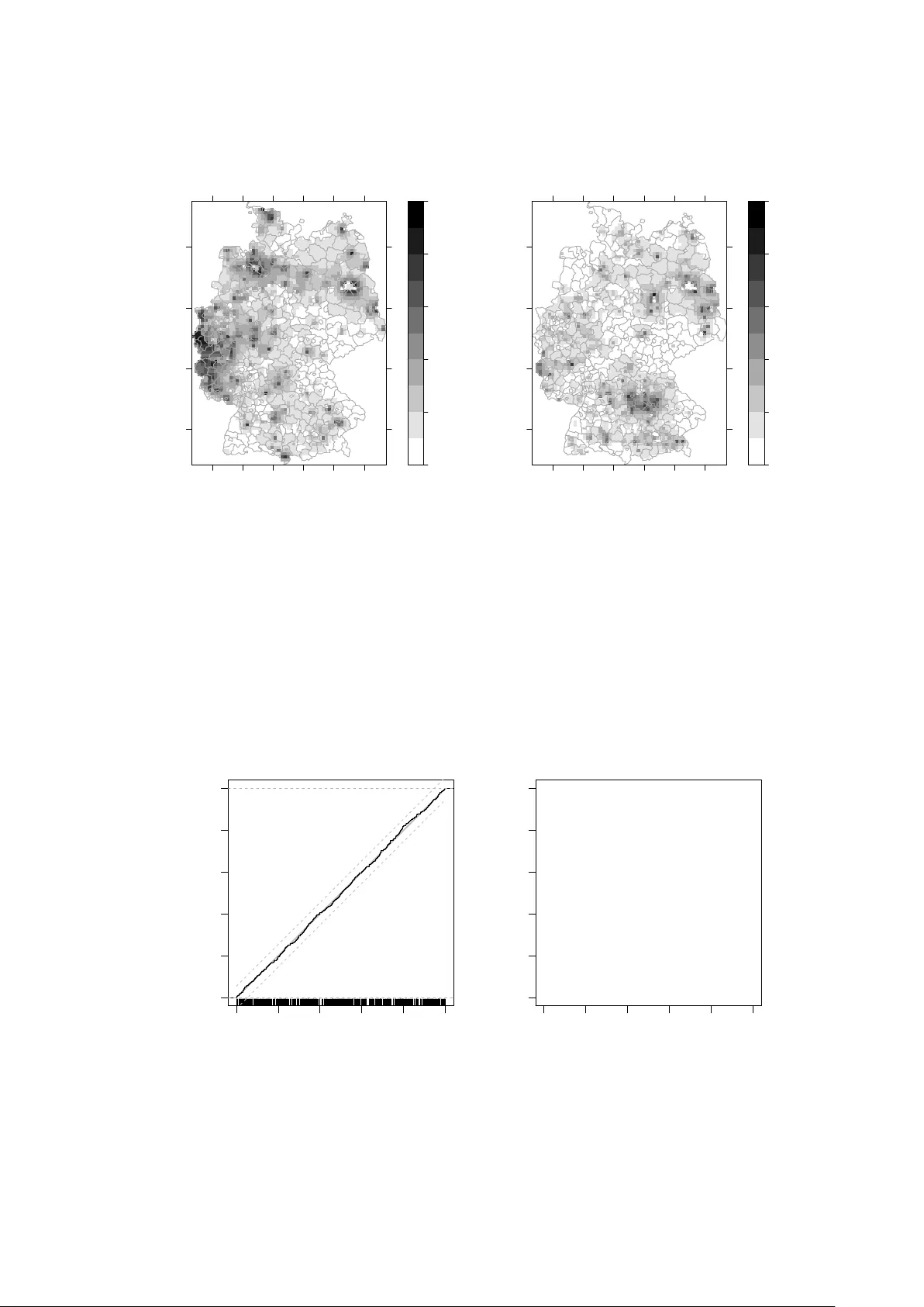
Spatio-T emp oral Analysis of Epidemic Phenomena Using the R P ac kage surv eillance Sebastian Mey er Univ ersity of Zurich Leonhard Held Univ ersity of Zurich Mic hael Höhle Sto c kholm Universit y Abstract The a v ailabilit y of geo coded health data and the inheren t temp oral structure of com- m unicable diseases ha v e led to an increased interest in statistical mo dels and softw are for spatio-temporal data with epidemic features. The open source R package surv eillance can handle v arious levels of aggregation at which infective even ts ha ve b een recorded: individual-lev el time-stamp ed geo-referenced data (case rep orts) in either con tinuous space or discrete space, as well as counts aggregated b y p erio d and region. F or eac h of these data t yp es, the surveillance package implements tools for visualization, lik eliho o o d infer- ence and simulation from recently developed statistical regression frameworks capturing endemic and epidemic dynamics. Altogether, this pap er is a guide to the spatio-temporal mo deling of epidemic phenomena, exempliﬁed by analyses of public health surveillance data on measles and inv asiv e meningo co ccal disease. K eywor ds : spatio-temp oral surv eillance data, endemic-epidemic mo deling, infectious disease epidemiology , self-exciting point pro cess, multiv ariate time series of counts, branching process with immigration. 1. In tro duction Epidemic data are realizations of spatio-temp oral pro cesses with autoregressive or “self- exciting” b eha vior. Examples of epidemic phenomena beyond infectious diseases include earth quakes ( Ogata 1999 ), crimes ( Johnson 2010 ; Mohler, Short, Brantingham, Schoenberg, and Tita 2011 ), in v asiv e sp ecies ( Balderama, Sc ho en b erg, Murra y , and R undel 2012 ), and forest ﬁres ( V rbik, Deardon, F eng, Gardner, and Braun 2012 ). Epidemic data are special with regard to at least three asp ects, which hinder the application of classical statistical ap- proac hes: the data are rarely a result of planned exp erimen ts, the observ ations (cases, even ts) are not indep endent, and often the pro cess is only partially observ able. 2 surv eillance : Spatio-T emp oral Analysis of Epidemic Phenomena Since 2005, the op en source R ( R Core T eam 2015 ) package surv eillance pro vides a gro w- ing computational framework for metho dological dev elopmen ts and practical to ols for the monitoring and mo deling of epidemic phenomena – traditionally in the con text of infec- tious diseases. Monitoring is concerned with prosp ective ab erration detection for whic h sev- eral algorithms hav e b een implemented as describ ed by Höhle ( 2007 ) and recen tly up dated and review ed by Salmon, Sc humac her, and Höhle ( 2015 ). The other ma jor purp ose of the surv eillance package and the fo cus of this pap er is the regression-orien ted mo deling of spatio- temp oral epidemic data. This enables the user to a) assess the role of environmen tal factors, so cio-demographic characteristics, or con trol measures in shaping endemic and epidemic dy- namics, b) analyze the spatio-temporal interaction of even ts, and c) sim ulate the epidemic spread from estimated mo dels. The implemen ted statistical modeling framew orks hav e already b een successfully applied to a broad range of surv eillance data, e.g., h uman inﬂuenza ( P aul, Held, and T oschk e 2008 ; Paul and Held 2011 ; Geilhufe, Held, Skrø vseth, Simonsen, and Go dtliebsen 2014 ), meningo co ccal disease ( P aul et al. 2008 ; P aul and Held 2011 ; Mey er, Elias, and Höhle 2012 ), measles ( Herzog, P aul, and Held 2011 ), psychiatric hospital admissions ( Mey er, W arnke, Rössler, and Held 2015 ), rabies in fo xes ( Höhle, Paul, and Held 2009 ), coxiellosis in cows ( Schrödle, Held, and R ue 2012 ), and the classical swine fev er virus ( Höhle 2009 ). Although these applications all originate from public or animal health surveillance, we stress that our metho ds also apply to the other epidemic phenomena describ ed ab ov e. T o the b est of our knowledge, no other softw are can estimate regression mo dels for spatio- temp oral epidemic data. There are, ho wev er, some related R packages that w e like to mention here, since they also deal with epidemic phenomena. F or instance, the R -epi pr oje ct 1 lists the pac kage EpiEstim ( Cori, F erguson, F raser, and Cauc hemez 2013 ), which can estimate the av erage num b er of secondary cases caused b y an infected individual, the so-called repro- duction num b er, from a time series of disease incidence. Similar functionalit y is provided by the package R0 ( Obadia, Haneef, and Bo elle 2012 ). Other pac kages are designed to estimate transmission characteristics from phylogenetic trees ( T reeP ar , Stadler and Bonho eﬀer 2013 ), or to reconstruct transmission trees from sequence data ( outbreaker , Jom bart, Cori, Didelot, Cauc hemez, F raser, and F erguson 2014 ). The pac kage amei ( Merl, Johnson, Gramacy , and Mangel 2010 ) is targeted to w ards ﬁnding optimal interv ention strategies, e.g., the prop ortion of the p opulation to b e v accinated to preven t further disease spread, using purely temp oral epidemic mo dels. The recently published package tscount ( Lib osc hik, F okianos, and F ried 2015 ) is dedicated to the analysis of coun t time series with serial correlation such as the n um- b er of sto c k mark et transitions p er min ute or the weekly n umber of rep orted infections of a particular disease. The tscoun t package can ﬁt a univ ariate v ersion of the areal count time- series mo del presen ted in Section 5 . F or a purely spatial analysis of disease o ccurrence, see, e.g., the recen t pap er by Brown ( 2015 ) introducing the package diseasemapping . One of the few packages ﬁtting spatio-temp oral epidemic mo dels is etasFLP ( A delﬁo and Chio di 2015 ). The Epidemic-Type Aftersho ck-Sequences (ET AS) mo del for earthquakes ( Ogata 1999 ) is closely related to the endemic-epidemic p oint process mo del describ ed in Section 3 , but incorp orates seismological la ws rather than co v ariates. The long-standing pac kage splancs ( Ro wlingson and Diggle 2015 ) oﬀers diagnostic to ols to inv estigate space-time clustering in a p oint pattern, i.e., to c heck if the pro cess at hand sho ws self-exciting epidemic b eha vior. Statistical tests for space-time in teraction are discussed in Meyer et al. ( 2015 ), who prop ose 1 https://sites.google.com/site/therepiproject/ Sebastian Meyer, Leonhard Held, Mic hael Höhle 3 a test based on the regression framew ork of Section 3 . An imp ortant recent dev elopmen t for spatio-temp oral tasks in R are the basic data classes and utilit y functions pro vided by the dedicated package spacetime ( Pebesma 2012 ), whic h builds up on the quasi standards sp ( Biv and, P eb esma, and Gómez-Rubio 2013 ) for spatial data and xts ( R yan and Ulrich 2014 ) for time-indexed data, respectively . F or a more general ov erview of R packages for spatio- temp oral data, see the CRAN T ask View “Handling and Analyzing Spatio-T emp oral Data” ( P eb esma 2015 ). A non- R option is the Sp atiotemp or al Epidemiolo gic al Mo deler (STEM) to ol 2 . It has a graphical user interface and can simulate the evolution of disease incidence in a p opulation. The abilit y to estimate mo del parameters from surveillance data, how ever, is limited to simple non-spatial models. WinBUGS has been used for Bay esian inference of spe- cialized spatio-temp oral epidemic mo dels ( Malesios, Demiris, Kalogerop oulos, and Ntzoufras 2014 ). The remainder of this pap er is organized as follows: Section 2 gives a brief o verview of the three statistical mo dels for spatio-temporal epidemic data implemented in surv eillance . Eac h of the subsequent mo del-sp eciﬁc Sections 3 to 5 ﬁrst describ es the asso ciated metho dology and then illustrates the model implementation – including data handling, visualization, inference, and simulation – by applications to infectious disease surv eillance data. Section 6 concludes the pap er. 2. Spatio-temp oral endemic-epidemic mo deling Epidemic mo dels traditionally describ e the spread of a communicable disease in a p opulation. Often, a compartmen tal view of the p opulation is tak en, placing individuals into one of the three states (S)usceptible, (I)nfectious, or (R)emov ed. Mo deling the transitions b etw een these states in a closed p opulation using deterministic diﬀerential equations dates back to the w ork of Kermac k and McKendric k ( 1927 ). Considering a sto c hastic v ersion of the simplest homogeneous SIR mo del in a closed p opulation of size N , the hazard rate for a susceptible individual i ∈ S ( t ) to b ecome infectious at time t – the so-called force of infection – is λ i ( t ) = X j ∈ I ( t ) β . (1) Here, S ( t ) , I ( t ) ⊆ { 1 , . . . , N } denote the index sets of currently susceptible and infectious indi- viduals, resp ectively , and the parameter β > 0 is called the transmission rate. The sto chastic SIR mo del is complemented by a distributional assumption ab out how long individuals are infectiv e, where t ypical choices are the exp onen tial or the gamma distribution. The set of reco vered individuals at time t is found as R ( t ) = { 1 , . . . , N } \ ( S ( t ) ∪ I ( t )) . The ab ov e homogeneous SIR mo del has since b een extended in a m ultitude of wa ys, e.g., by additional states (addressing population heterogeneities arising from age groups, spatial lo cation or v ac- cination) or p opulation demographics. Overviews of SIR mo deling approaches can b e found in Anderson and Ma y ( 1991 ), Daley and Gani ( 1999 ), and Keeling and Rohani ( 2008 ). The estimation of SIR mo del parameters from actual observ ed data is, how ever, often only treated marginally in such descriptions. In contrast, a n umber of more statistically ﬂa vored epidemic mo dels ha ve emerged recently . This includes, e.g., the TSIR model ( Fink enstädt and Grenfell 2000 ), tw o-comp onent time-series models ( Held, Höhle, and Hofmann 2005 ; Held, Hofmann, 2 https://www.eclipse.org/stem/ 4 surv eillance : Spatio-T emp oral Analysis of Epidemic Phenomena Höhle, and Schmid 2006 ), and p oint pro cess models ( La wson and Leimich 2000 ; Diggle 2006 ). An ov erview of temp oral and spatio-temp oral epidemic mo dels and their relation to the un- derlying metap opulation SIR mo dels can b e found in Höhle ( 2016 ). A t the heart of any statistical analysis is the sub ject-matter scientiﬁc problem, whic h a data- driv en analysis seeks to address. Due to the generality and complexity of such problems we adopt here a technocratic view and let the a v ailable data guide what a “useful” epidemic mo del is. The surv eillance package oﬀers regression-oriented mo deling frameworks for three diﬀeren t t yp es of spatio-temp oral data distinguished by the spatial and temp oral resolution (T able 1 ). First, if an entire region is contin uously monitored for infective ev en ts, which are time-stamp ed, geo-referenced, and p otentially enriched with further even t-sp eciﬁc data, then a (mark ed) spatio-temp oral p oin t pattern arises. Such contin uous space-time epidemic data can b e view ed as a realization of a self-exciting spatio-temp oral p oint pro cess (Section 3 ). The second data type we consider comprises the ev ent history of a discrete set of units follow ed o ver time – e.g., farms during liv esto c k epidemics – while registering when they become susceptible, infected, and potentially remov ed (neither at risk nor infectious). These data ﬁt into the framew ork of a spatial SIR mo del represented as a multiv ariate temp oral p oin t pro cess (Section 4 ). Our third data type is often encountered as a result of priv acy protection or rep orting regimes, and is an aggregated version of the individual even t data mentioned ﬁrst: ev ent counts b y region and p erio d. Suc h areal count time series can b e ﬁtted with the m ultiv ariate negative binomial time-series mo del presented in Section 5 . The three aforemen tioned mo del classes are all inspired by the P oisson branching pro cess with immigration approach prop osed by Held et al. ( 2005 ). Its main characteristic is the additiv e decomposition of disease risk in to endemic and epidemic features, similar to the b ackgr ound and trigger e d components in the ET AS mo del for earthquake o ccurrence. The endemic comp onen t describ es the risk of new ev en ts by external factors indep endent of the history of the epidemic pro cess. In the context of infectious diseases, such factors ma y in- clude seasonalit y , p opulation densit y , so cio-demographic v ariables, and v accination cov erage – all p otentially v arying in time and/or space. Explicit dependence b et ween ev ents is then in tro duced through an epidemic component driv en b y the observ ed past. Eac h of the following three mo del-sp eciﬁc sections starts with a brief theoretical introduction to the resp ective spatio-temporal endemic-epidemic mo del, b efore we describe the implemen- tation using the example data men tioned in T able 1 . twinstim (Section 3 ) twinSIR (Section 4 ) hhh4 (Section 5 ) Data class epidataCS epidata sts Resolution individual even ts in individual SI[R][S] even t ev ent coun ts aggregated con tinuous space-time history of a ﬁxed p opulation b y region and time p erio d Example cases of meningo co ccal measles outbreak among w eekly coun ts of measles b y disease, Germany , 2002–8 c hildren in Hagello ch, 1861 district, W eser-Ems, 2001–2 Mo del (mark ed) spatio-temporal m ultiv ariate temporal m ultiv ariate time series p oin t pro cess p oin t pro cess (P oisson or NegBin) Reference Mey er et al. ( 2012 ) Höhle ( 2009 ) Held and Paul ( 2012 ) T able 1: Spatio-temp oral endemic-epidemic mo dels and corresponding data classes imple- men ted in the R package surveillance . Sebastian Meyer, Leonhard Held, Mic hael Höhle 5 3. Spatio-temp oral p oin t pattern of infectiv e even ts The endemic-epidemic spatio-temp oral point pro cess mo del “ twinstim ” is designed for p oint- referenced, individual-lev el surveillance data. As an illustrative example, w e use case rep orts of inv asive meningoco ccal disease (IMD) caused by the tw o most common bacterial ﬁnet yp es of meningo co cci in Germany , 2002–2008, as previously analyzed b y Meyer et al. ( 2012 ) and Mey er and Held ( 2014a ). W e start by describing the general mo del class in Section 3.1 . Sec- tion 3.2 in tro duces the example data and the asso ciated class epidataCS , Section 3.3 presen ts the core functionalit y of ﬁtting and analyzing such data using twinstim , and Section 3.4 shows ho w to sim ulate realizations from a ﬁtted mo del. 3.1. Mo del class: twinstim Infectiv e even ts o ccur at speciﬁc p oints in contin uous space and time, which gives rise to a spatio-temp oral p oin t pattern { ( s i , t i ) : i = 1 , . . . , n } from a region W observ ed during a p erio d (0 , T ] . The lo cations s i and time p oin ts t i of the n even ts can b e regarded as a realization of a self-exciting spatio-temp oral p oint pro cess, which can b e c haracterized b y its conditional intensit y function (CIF, also termed intensit y pro cess) λ ( s , t ) . It represents the instan taneous ev en t rate at lo cation s at time p oint t giv en all past even ts, and is often more v erb osely denoted b y λ ∗ or b y explicit conditioning on the “history” H t of the process. Daley and V ere-Jones ( 2003 , Chapter 7) provide a rigorous mathematical deﬁnition of this concept, whic h is k ey to likelihoo d analysis and simulation of “evolutionary” p oin t pro cesses. Mey er et al. ( 2012 ) formulated the mo del class “ twinstim ” – a two -comp onent s patio- t emp oral i ntensit y m o del – b y a sup erp osition of an endemic and an epidemic comp onent: λ ( s , t ) = ν [ s ][ t ] + X j ∈ I ( s ,t ) η j f ( k s − s j k ) g ( t − t j ) . (2) This mo del constitutes a branc hing pro cess with immigration, where part of the even t rate is due to the ﬁrst, endemic comp onen t, whic h reﬂects sporadic even ts caused by unobserved sources of infection. This background rate of new ev ents is mo delled by a piecewise constant log-linear predictor ν [ s ][ t ] incorp orating regional and/or time-v arying c haracteristics. Here, the space-time index [ s ][ t ] refers to the region co vering s during the p erio d con taining t and th us spans a whole spatio-temp oral grid on whic h the inv olved cov ariates are measured, e.g., district × mon th. W e will later see that the endemic comp onent therefore simply equals an inhomogeneous Poisson pro cess for the ev en t coun ts b y cell of that grid. The second, observ ation-driven epidemic comp onent adds “infection pressure” from the set I ( s , t ) =  j : t j < t ∧ t − t j ≤ τ j ∧ k s − s j k ≤ δ j  of past even ts and hence mak es the process “self-exciting” . During its infectious perio d of length τ j and within its spatial in teraction radius δ j , the mo del assumes each ev en t j to trigger furth er even ts, which are called oﬀspring, secondary cases, or aftersho c ks, dep ending on the application. The triggering rate (or force of infection) is prop ortional to a log-linear predictor η j asso ciated with even t-sp eciﬁc characteristics (“marks”) m j , whic h are usually attac hed to the point pattern of even ts. The deca y of infection pressure with increasing spatial and temp oral distance from the infective even t is mo delled by parametric interaction functions f and g , resp ectiv ely ( La wson and Leimich 2000 , Section 4). A simple assumption 6 surv eillance : Spatio-T emp oral Analysis of Epidemic Phenomena for the time course of infectivit y is g ( t ) = 1 . Alternativ es include exp onential deca y , a step function, or empirically derived functions such as Omori’s law for aftersho ck in terv als ( Utsu, Ogata, and Matsu’ura 1995 ). With regard to spatial in teraction, the statistician’s standard c hoice is a Gaussian k ernel f ( x ) = exp  − x 2 / (2 σ 2 )  . Ho wev er, in modeling the spread of h uman infectious diseases on larger scales, a heavy-tailed p ow er-law kernel f ( x ) = ( x + σ ) − d w as found to p erform b etter ( Mey er and Held 2014a ). The (p ossibly inﬁnite) upp er b ounds τ j and δ j pro vide a w ay of mo deling ev en t-sp eciﬁc in teraction ranges. How ever, since these need to b e pre-sp eciﬁed, a common assumption is τ j ≡ τ and δ j ≡ δ , where the infectious p erio d τ and the spatial interaction radius δ are determined b y sub ject-matter considerations. Mo del-b ase d eﬀe ctive r epr o duction numb ers Similar to the simple SIR mo del (see, e.g., Keeling and Rohani 2008 , Section 2.1), the ab ov e p oin t pro cess mo del ( 2 ) features a repro duction n um b er deriv ed from its branching pro cess in terpretation. As so on as an ev ent o ccurs (individual b ecomes infected), it triggers oﬀspring (secondary cases) around its origin ( s j , t j ) according to an inhomogeneous Poisson pro cess with rate η j f ( k s − s j k ) g ( t − t j ) . Since this triggering pro cess is indep endent of the even t’s paren tage and of other even ts, the exp ected num b er µ j of ev ents triggered by even t j can b e obtained by integrating the triggering rate ov er the observed interaction domain: µ j = η j · " Z min( T − t j ,τ j ) 0 g ( t ) dt # · " Z R j f ( k s k ) d s # , (3) where R j = ( b ( s j , δ j ) ∩ W ) − s j (4) is ev en t j ’s inﬂuence region centered at s j , and b ( s j , δ j ) denotes the disc centered at s j with radius δ j . Note that the ab ov e mo del-based repro duction num b er µ j is even t-sp eciﬁc since it dep ends on even t marks through η j , on the ranges of interaction δ j and τ j , as well as on the ev ent lo cation s j and time p oint t j . Equation 3 can also b e motiv ated b y lo oking at a spatio-temp oral version of the simple SIR mo del ( 1 ) wrapp ed in to the twinstim class ( 2 ). This means: no endemic comp onent, homogeneous force of infection ( η j ≡ β ), homogeneous mixing in space ( f ( x ) = 1 , δ j ≡ ∞ ), and exp onential decay of infectivit y ( g ( t ) = e − αt , τ j ≡ ∞ ). Then, for T → ∞ , µ = β ·  Z ∞ 0 e − αt dt  · " Z W − s j 1 d s # = β · | W | /α , whic h correspond s to the basic repro duction n umber known from the simp le SIR mo del by in terpreting | W | as the population size, β as the transmission rate and α as the remov al rate. Lik e in classic epidemic mo dels, the pro cess is sub-critical if µ < 1 holds, which means that its even tual extinction is almost sure. Ho wev er, it is crucial to understand that in a full mo del with an endemic comp onent, new infections may alw a ys o ccur via “immigration” . Hence, repro duction n umbers in twinstim are adjusted for infections o ccurring indep endently of previous infections. This also means that a missp eciﬁed endemic comp onent may distort mo del-based repro duction num b ers ( Mey er et al. 2015 ). F urthermore, under-rep orting and implemen ted con trol measures imply that the estimates are to b e though t of as eﬀe ctive repro duction n umbers. Sebastian Meyer, Leonhard Held, Mic hael Höhle 7 Likeliho o d infer enc e The log-likelihoo d of the p oint pro cess mo del ( 2 ) is a function of all parameters in the log- linear predictors ν [ s ][ t ] and η j and in the in teraction functions f and g . It has the form " n X i =1 log λ ( s i , t i ) # − Z T 0 Z W λ ( s , t ) d s d t . (5) T o estimate the mo del parameters, w e maximize the ab ov e log-likelihoo d n umerically using the quasi-Newton algorithm av ailable through the R function nlminb . W e thereb y make use of the analytical score function and an approximation of the exp ected Fisher information w orked out by Meyer et al. ( 2012 , W eb App endices A and B). The space-time integral in the log-lik eliho o d poses no diﬃculties for the endemic comp onen t of λ ( s , t ) since it is piecewise constant. Ho wev er, in tegration of the epidemic component has a clear computational b ottleneck: t w o-dimensional integrals R R i f ( k s k ) d s o ver the inﬂuence regions R i of Equation 4 , whic h are computationally represen ted b y p olygons (as is W ). Similar integrals appear in the score function, where f ( k s k ) is replaced by partial deriv ativ es with resp ect to kernel parameters, e.g., ∂ f ( k s k ) /∂ log σ for the Gaussian kernel with standard deviation estimated on the log-scale. Calculation of these integrals is trivial for (piecewise) constan t f , but otherwise requires n umerical integration. F or this purp ose, the R package p olyCub ( Meyer 2015 ) oﬀers cubature metho ds for p olygonal domains as describ ed in Meyer and Held ( 2014b , Section 2). F or Gaussian f , we apply the tw o-dimensional midp oint rule with a σ -adaptive bandwidth, combined with an analytical formula via the χ 2 distribution if the 6 σ - circle around s i is con tained in R i ( Mey er et al. 2012 ). The in tegrals in the score function are appro ximated by pro duct Gauss cubature ( Sommariv a and Vianello 2007 ). F or the recen tly implemen ted p o wer-la w kernels ( Meyer and Held 2014a ), we apply a particularly app ealing metho d which takes analytical adv an tage of the assumed isotrop y of spatial interaction in suc h a wa y that numerical integration remains in only one dimension ( Meyer and Held 2014b , Section 2.4). As a general means to reduce the computational burden during numerical log- lik eliho o d maximization, we memoise ( Wickham 2014 ) the cubature function, which av oids redundan t re-ev aluations of the integral with identical parameters of f . Sp e cial c ase: Endemic-only twinstim As men tioned abov e, a twinstim mo del without an epidemic comp onent can actually b e represen ted as a Poisson regression mo del for aggregated counts. This provides a nice link to ecological regression approaches in general ( W aller and Gotw ay 2004 ) and to the coun t data mo del hhh4 illustrated in Section 5 . T o see this, recall that the endemic comp onent ν [ s ][ t ] of a twinstim ( 2 ) is piecewise constan t on the spatio-temp oral grid with cells ([ s ] , [ t ]) . Hence the log-likelihoo d ( 5 ) of an endemic-only twinstim simpliﬁes to a sum ov er all these cells, X [ s ] , [ t ] n Y [ s ][ t ] log ν [ s ][ t ] − | [ s ] | | [ t ] | ν [ s ][ t ] o , where Y [ s ][ t ] is the aggregated n umber of even ts observed in cell ([ s ] , [ t ]) , and | [ s ] | and | [ t ] | denote cell area and length, resp ectively . Except for an additiv e constan t, the ab ov e log- lik eliho o d is equiv alen tly obtained from the Poisson mo del Y [ s ][ t ] ∼ P o( | [ s ] | | [ t ] | ν [ s ][ t ] ) . This relation oﬀers a means of co de v alidation using the established glm function to ﬁt an endemic- only twinstim mo del, see the examples in help("glm_epidataCS") . 8 surv eillance : Spatio-T emp oral Analysis of Epidemic Phenomena Extension: twinstim with event typ es T o mo del the example data on in v asiv e meningo co ccal disease in the remainder of this sec- tion, we actually need to use an extended v ersion λ ( s , t, k ) of Equation 2 , which accoun ts for diﬀeren t even t types k with own transmission dynamics. This introduces a further dimension in the p oin t pro cess, and the second log-likelihoo d comp onen t in Equation 5 accordingly splits in to a sum ov er all even t t yp es. W e refer to Mey er et al. ( 2012 , Sections 2.4 and 3) for the tec hnical details of this type-sp eciﬁc twinstim class. The basic idea is that the meningo co ccal ﬁnet yp es share the same endemic pattern (e.g., seasonality), while infections of diﬀerent ﬁne- t yp es are not asso ciated via transmission. This means that the force of infection is restricted to previously infected individuals with the same bacterial ﬁnet yp e k , i.e., the epidemic sum in Equation 2 is o ver the set I ( s , t, k ) = I ( s , t ) ∩ { j : k j = k } . The implemen tation has limited supp ort for type-dep endent in teraction functions f k j and g k j (not further considered here). 3.2. Data structure: epidataCS The ﬁrst step to ward ﬁtting a twinstim is to turn the relev ant data into an ob ject of the dedicated class epidataCS . 3 The primary ingredients of this class are a spatio-temporal p oin t pattern ( events ) and its underlying observ ation region ( W ). An additional spatio-temp oral grid ( stgrid ) holds (time-v arying) areal-lev el cov ariates for the endemic regression part. W e exemplify this data class b y the epidataCS ob ject for the 636 cases of in v asiv e meningo co ccal disease in Germany originally analyzed b y Meyer et al. ( 2012 ). It is already con tained in the surv eillance pac kage as data("imdepi") and has b een constructed as follows: R> imdepi <- as.epidataCS(events = events, W = stateD, stgrid = stgrid, + qmatrix = diag(2), nCircle2Poly = 16) The function as.epidataCS c hecks the consistency of the three data ingredien ts describ ed in detail b elow. It also pre-computes auxiliary v ariables for mo del ﬁtting, e.g., the individual in- ﬂuence regions ( 4 ), which are in tersections of the observ ation region with discs approximated b y p olygons with nCircle2Poly = 16 edges. The intersections are computed using function- alit y of the package p olyclip ( Johnson 2015 ). F or m ultit yp e epidemics as in our example, the additional indicator matrix qmatrix sp eciﬁes transmissibility across even t types. An iden tity matrix corresp onds to an indep endent spread of the even t types, i.e., cases of one type can not pro duce cases of another type. Data ingr e dients The core events data must b e provided in the form of a SpatialPointsDataFrame as deﬁned b y the pac kage sp ( Biv and et al. 2013 ): R> summary(events) Object of class SpatialPointsDataFrame Coordinates: min max x 4039 4665 y 2710 3525 3 The suﬃx “CS” indicates that the data-generating point pro cess is indexed in contin uous space. Sebastian Meyer, Leonhard Held, Mic hael Höhle 9 Is projected: TRUE proj4string : [+init=epsg:3035 +units=km +proj=laea +lat_0=52 +lon_0=10 +x_0=4321000 +y_0=3210000 +ellps=GRS80 +no_defs] Number of points: 636 Data attributes: time tile type eps.t eps.s sex agegrp Min. : 0 05354 : 34 B:336 Min. :30 Min. :200 female:292 [0,3) :194 1st Qu.: 539 05370 : 27 C:300 1st Qu.:30 1st Qu.:200 male :339 [3,19) :279 Median :1155 11000 : 27 Median :30 Median :200 NA ' s : 5 [19,Inf):162 Mean :1193 05358 : 13 Mean :30 Mean :200 NA ' s : 1 3rd Qu.:1808 05162 : 12 3rd Qu.:30 3rd Qu.:200 Max. :2543 05382 : 12 Max. :30 Max. :200 (Other):511 The asso ciated even t co ordinates are residence p ostco de cen troids, pro jected in the Eur op e an T err estrial R efer enc e System 1989 (in kilometer units) to enable Euclidean geometry . See the spTransform -metho ds in pac kage rgdal ( Biv and, Keitt, and Rowlingson 2015 ) for how to pro ject latitude and longitude co ordinates in to a planar co ordinate reference system (CRS). The data frame asso ciated with these spatial co ordinates ( s i ) contains a n um b er of required v ariables and additional even t marks (in the notation of Section 3.1 : { ( t i , [ s i ] , k i , τ i , δ i , m i ) : i = 1 , . . . , n } ). F or the IMD data, th e even t time is measured in da ys since the beginning of the observ ation perio d 2002–2008 and is sub ject to a tie-breaking pro cedure (describ ed later). The tile column refers to the region of the spatio-temp oral grid where the even t o ccurred and here contains the oﬃcial key of the administrative district of the patient’s residence. There are tw o type s of ev en ts labeled as "B" and "C" , which refer to the serogroups of the t wo meningo co ccal ﬁnetypes B:P1.7-2,4:F1-5 and C:P1.5,2:F3-3 con tained in the data. The eps.t and eps.s columns specify upp er limits for temporal and spatial in teraction, resp ectiv ely . Here, the infectious perio d is assumed to last a maximum of 30 days and spatial in teraction is limited to a 200 km radius for all cases. The latter has numerical ad v an tages for a Gaussian interaction function f with a relativ ely small standard deviation. F or a p o wer-la w k ernel, how ever, this restriction will b e dropp ed to enable occasional long-range transmission. The last tw o data attributes display ed in the ab ov e event summary are cov ariates from the case rep orts: the gender and age group of the patient. F or the observ ation region W , w e use a p olygon represen tation of Germany’s b oundary . Since the observ ation region deﬁnes the integration domain in the p oint pro cess log-likelihoo d ( 5 ), the more detailed the p olygons of W are the longer it will tak e to ﬁt a twinstim . It is thus advisable to sacriﬁce some shap e details for sp eed by reducing the p olygon complexity , e.g., by applying one of the simpliﬁcation metho ds a v ailable at MapShap er.org ( Harrow er and Blo c h 2006 ). Alternativ e to ols in R are spatstat ’s simplify.owin pro cedure ( Baddeley , R ubak, and T urner 2015 ) and the function thinnedSpatialPoly in package mapto ols ( Biv and and Lewin-K oh 2015 ), which implemen ts the Douglas and P euck er ( 1973 ) reduction metho d. The surv eillance pac kage already con tains a simpliﬁed representation of German y’s b oundaries: R> load(system.file("shapes", "districtsD.RData", package = "surveillance")) This ﬁle con tains b oth the SpatialPolygonsDataFrame districtsD of German y’s 413 ad- ministrativ e districts as at January 1, 2009, as w ell as their union stateD . These b oundaries are pro jected in the same CRS as the events data. 10 surv eillance : Spatio-T emp oral Analysis of Epidemic Phenomena The stgrid input sp eciﬁc to the endemic mo del component is a simple data frame with (time-dep enden t) areal-level co v ariates, e.g., so cio-economic or ecological c haracteristics. F or our IMD example, we ha ve: start stop tile area popdensity 1 0 31 01001 56.4 1557.1 2 0 31 01002 118.7 1996.6 3 0 31 01003 214.2 987.6 ... ... ... ... ... ... 34690 2526 2557 16075 1148.5 79.2 34691 2526 2557 16076 843.5 133.6 34692 2526 2557 16077 569.1 181.5 Numeric ( start , stop ] columns index the time p erio ds and the factor v ariable tile identiﬁes the regions of the grid. Note that the given time interv als (here: mon ths) also deﬁne the resolution of p ossible time trends and seasonalit y of the piecewise constant endemic in tensity . W e choose mon thly in terv als to reduce package size and computational cost compared to the w eekly resolution originally used by Meyer et al. ( 2012 ) and Meyer and Held ( 2014a ). The ab o v e stgrid data frame th us consists of 7 (years) times 12 (mon ths) blo c ks of 413 (districts) ro ws eac h. The area column giv es the area of the resp ective tile in square kilometers (compatible with the CRS used for events and W ). A geographic represen tation of the regions in stgrid is not required for mo del estimation, and is th us not part of the epidataCS class. In our example, the areal-lev el data only consists of the p opulation density popdensity , whereas Mey er et al. ( 2012 ) additionally incorporated (lagged) weekly inﬂuenza counts by district as a time-dep endent cov ariate. Data hand ling and visualization The generated epidataCS ob ject imdepi is a simple list of the chec k ed ingredients events , stgrid , W and qmatrix . Sev eral metho ds for data handling and visualization are av ailable for such ob jects as listed in T able 2 and brieﬂy presented in the remainder of this section. Prin ting an epidataCS ob ject presents some metadata and the ﬁrst 6 even ts by default: R> imdepi Observation period: 0 - 2557 Observation window (bounding box): [4031, 4672] x [2684, 3550] Spatio-temporal grid (not shown): 84 time blocks x 413 tiles Types of events: "B" "C" Overall number of events: 636 coordinates time tile type eps.t eps.s sex agegrp BLOCK start popdensity 1 (4110, 3200) 0.212 05554 B 30 200 male [3,19) 1 0 261 2 (4120, 3080) 0.712 05382 C 30 200 male [3,19) 1 0 519 3 (4410, 2920) 5.591 09574 B 30 200 female [19,Inf) 1 0 209 4 (4200, 2880) 7.117 08212 B 30 200 female [3,19) 1 0 1666 5 (4130, 3220) 22.060 05554 C 30 200 male [3,19) 1 0 261 6 (4090, 3180) 24.954 05170 C 30 200 male [3,19) 1 0 455 [....] Sebastian Meyer, Leonhard Held, Mic hael Höhle 11 During con v ersion to epidataCS , the last three columns BLOCK (time in terv al index), start and popdensity hav e been merged from the c hec ked stgrid to the events data frame. The even t marks including time and lo cation can b e extracted in a standard data frame by marks(imdepi) , and this is summarized b y summary(imdepi) . Displa y Subset Extract Mo dify Con v ert print [ nobs update as.epidata summary head marks untie epidataCS2sts plot tail animate subset as.stepfun T able 2: Generic and non-generic functions applicable to epidataCS ob jects. A simple plot of the num b er of infectives as a function of time (Figure 1 ) can b e obtained b y the step function conv erter: R> plot(as.stepfun(imdepi), xlim = summary(imdepi)$timeRange, xaxs = "i", + xlab = "Time [days]", ylab = "Current number of infectives", main = "") 0 500 1000 1500 2000 2500 0 5 10 15 20 Time [days] Current number of inf ectives Figure 1: Time course of the n umber of infectiv es assuming infectious p erio ds of 30 days. The plot -metho d for epidataCS oﬀers aggregation of the ev ents ov er time or space: R> plot(imdepi, "time", col = c("indianred", "darkblue"), ylim = c(0, 20)) R> plot(imdepi, "space", lwd = 2, + points.args = list(pch = c(1, 19), col = c("indianred", "darkblue"))) R> layout.scalebar(imdepi$W, scale = 100, labels = c("0", "100 km"), plot = TRUE) The time-series plot (Figure 2a ) shows the monthly aggregated n umber of cases b y ﬁnet yp e in a stack ed histogram as w ell as each t yp e’s cum ulative n umber o ver time. The spatial plot (Figure 2b ) shows the observ ation window W with the lo cations of all cases (by type), where the areas of the p oints are proportional to the n um b er of cases at the respective lo cation. A d- ditional shading by the population is p ossible and exempliﬁed in help("plot.epidataCS") . 12 surv eillance : Spatio-T emp oral Analysis of Epidemic Phenomena 0 500 1000 1500 2000 2500 0 5 10 15 20 Time Number of cases 0 84 168 252 336 Cumulativ e number of cases type B C (a) T emp oral pattern. ● ● ● ● ● ● ● ● ● ● ● ● ● ● ● ● ● ● ● ● ● ● ● ● ● ● ● ● ● ● ● ● ● ● ● ● ● ● ● ● ● ● ● ● ● ● ● ● ● ● ● ● ● ● ● ● ● ● ● ● ● ● ● ● ● ● ● ● ● ● ● ● ● ● ● ● ● ● ● ● ● ● ● ● ● ● ● ● ● ● ● ● ● ● ● ● ● ● ● ● ● ● ● ● ● ● ● ● ● ● ● ● ● ● ● ● ● ● ● ● ● ● ● ● ● ● ● ● ● ● ● ● ● ● ● ● ● ● ● ● ● ● ● ● ● ● ● ● ● ● ● ● ● ● ● ● ● ● ● ● ● ● ● ● ● ● ● ● ● ● ● ● ● ● ● ● ● ● ● ● ● ● ● ● ● ● ● ● ● ● ● ● ● ● ● ● ● ● ● ● ● ● ● ● ● ● ● ● ● ● ● ● ● ● ● ● ● ● ● ● ● ● ● ● ● ● ● ● ● ● ● ● ● ● ● ● ● ● ● ● ● ● ● ● ● ● ● ● ● ● ● ● ● ● ● ● ● ● ● ● ● ● ● ● ● ● ● ● ● ● ● ● ● ● ● ● ● ● ● ● ● ● ● ● ● ● ● ● ● ● ● ● ● ● ● ● ● ● ● ● ● ● ● ● ● ● ● ● ● ● ● ● ● ● ● ● ● ● ● ● ● ● ● ● ● ● ● ● ● ● ● ● ● ● ● ● ● ● ● ● ● ● ● ● ● ● ● ● ● ● ● ● ● ● ● ● ● ● ● ● ● ● ● ● ● ● ● ● ● ● ● ● ● ● ● ● ● ● ● ● ● ● ● ● ● ● ● ● ● ● ● ● ● ● ● ● ● ● ● ● ● ● ● ● ● ● ● ● ● ● ● ● ● ● ● ● ● ● ● ● ● ● ● ● ● ● ● ● ● ● ● ● ● ● ● ● ● ● ● ● ● ● ● ● ● ● ● ● ● ● ● ● ● ● ● ● ● ● ● ● ● ● ● ● ● ● ● ● ● ● ● ● ● ● ● ● ● ● ● ● ● ● ● ● ● ● ● ● ● ● ● ● ● ● ● ● ● ● ● ● ● ● ● ● ● ● ● ● ● ● ● ● ● ● ● ● ● ● ● ● ● ● ● ● ● ● ● ● ● ● ● ● ● ● ● ● ● ● ● type B C ● ● ● ● ● 1 2 4 8 16 0 100 km (b) Spatial pattern. Figure 2: Occurrence of the tw o ﬁnetypes view ed in the temp oral and spatial dimensions. The abov e static plots do not capture the space-time dynamics of epidemic spread. An animation may pro vide additional insight and can b e pro duced b y the corresp onding animate - metho d. F or instance, to lo ok at the ﬁrst y ear of the B-type in a w eekly sequence of snapshots in a web browser (using facilities of the animation pac kage of Xie 2013 ): R> animation::saveHTML( + animate(subset(imdepi, type == "B"), interval = c(0, 365), time.spacing = 7), + nmax = Inf, interval = 0.2, loop = FALSE, + title = "Animation of the first year of type B events") Selecting ev ents from epidataCS as for the animation ab ov e is enabled by the [ - and subset - metho ds, which return a new epidataCS ob ject containing only the selected events . A limited data sampling resolution may lead to tied even t times or lo cations, whic h are in conﬂict with a contin uous spatio-temp oral p oin t pro cess mo del. F or instance, a temp oral residual analysis would suggest mo del deﬁciencies ( Mey er et al. 2012 , Figure 4), and a p ow er- la w kernel for spatial interaction ma y diverge if there are even ts with zero distance to p otential source ev ents ( Meyer and Held 2014a ). The function untie breaks ties by random shifts. This has already b een applied to the even t times in the pro vided imdepi data by s ubtracting a U(0,1)-distributed random n umber from the original dates. The even t c o or dinates in the IMD data are sub ject to interv al censoring at the level of German y’s postco de regions. A p ossible replacemen t for the given centroids w ould thus b e a random lo cation within the corresp onding p ostco de area. Lac king a suitable shap eﬁle, Meyer and Held ( 2014a ) shifted all lo cations b y a random vector with length up to half the observ ed minim um spatial separation: Sebastian Meyer, Leonhard Held, Mic hael Höhle 13 R> eventDists <- dist(coordinates(imdepi$events)) R> (minsep <- min(eventDists[eventDists > 0])) [1] 1.17 R> set.seed(321) R> imdepi_untied <- untie(imdepi, amount = list(s = minsep / 2)) Note that random tie-breaking requires sensitivit y analyses as discussed by Meyer and Held ( 2014a ), but skipp ed here for the sake of brevit y . The update -metho d is useful to change the v alues of the maxim um interaction ranges eps.t and eps.s , since it takes care of the necessary up dates of the hidden auxiliary v ariables in an epidataCS ob ject. F or an un b ounded in teraction radius: R> imdepi_untied_infeps <- update(imdepi_untied, eps.s = Inf) Last but not least, epidataCS can b e conv erted to the other classes epidata (Section 4 ) and sts (Section 5 ) by aggregation. The metho d as.epidata.epidataCS aggregates even ts by region ( tile ), and the function epidataCS2sts yields counts b y region and time interv al. The data could then, e.g., b e analyzed b y the m ultiv ariate time-series mo del presen ted in Section 5 . W e can also use visualization to ols of the sts class, e.g., to pro duce Figure 3 : R> imdsts <- epidataCS2sts(imdepi, freq = 12, start = c(2002, 1), tiles = districtsD) R> plot(imdsts, type = observed ~ time) R> plot(imdsts, type = observed ~ unit, population = districtsD$POPULATION / 100000) time No . infected 2002 1 2004 1 2006 1 2008 1 0 2 4 6 8 10 12 14 16 18 (a) Time series of monthly coun ts. 2002/1 − 2008/12 0.00 2.25 4.00 6.25 9.00 12.25 (b) Disease incidence (p er 100 000 inhabitan ts). Figure 3: IMD cases (joint types) aggregated as an sts object b y mon th and district. 14 surv eillance : Spatio-T emp oral Analysis of Epidemic Phenomena 3.3. Mo deling and inference Ha ving prepared the data as an ob ject of class epidataCS , the function twinstim can be used to perform likelihoo d inference for conditional intensit y mo dels of the form ( 2 ). The main argumen ts for twinstim are the form ulae of the endemic and epidemic linear predictors ( ν [ s ][ t ] = exp ( endemic ) and η j = exp ( epidemic )), and the spatial and temp oral in teraction functions siaf ( f ) and tiaf ( g ), resp ectively . Both formulae are parsed internally using the standard model.frame to olb ox from pac kage stats and th us can handle factor v ariables and in teraction terms. While the endemic linear predictor incorp orates time-dep endent and/or areal-lev el cov ariates from stgrid , the epidemic form ula may use b oth stgrid v ariables and ev ent marks to b e asso ciated with the force of infection. F or the interaction functions, several alternativ es are predeﬁned as listed in T able 3 . They are applicable out-of-the-b ox and illus- trated as part of the follo wing mo deling exercise for the IMD data. Own interaction functions can also b e used provided their implemen tation ob eys a certain structure, see help("siaf") and help("tiaf") , resp ectively . Spatial ( siaf.* ) T emp oral ( tiaf.* ) constant constant gaussian exponential powerlaw step powerlawL step student T able 3: Predeﬁned spatial and temp oral interaction functions. Basic example T o illustrate statistical inference with twinstim , we will estimate sev eral mo dels for the simpliﬁed and “untied” IMD data presented in Section 3.2 . In the endemic comp onent, we include the district-speciﬁc p opulation density as a m ultiplicative oﬀset, a (centered) time trend, and a sin usoidal wa ve of frequency 2 π / 365 to capture seasonality , where the start v ariable from stgrid measures time: R> (endemic <- addSeason2formula(~offset(log(popdensity)) + I(start / 365 - 3.5), + period = 365, timevar = "start")) ~offset(log(popdensity)) + I(start/365 - 3.5) + sin(2 * pi * start/365) + cos(2 * pi * start/365) See Held and Paul ( 2012 , Section 2.2) for how suc h sine/cosine terms reﬂect seasonalit y . Because of the aforementioned in tegrations in the log-lik eliho o d ( 5 ), it is advisable to ﬁrst ﬁt an endemic-only mo del to obtain reasonable start v alues for more complex epidemic mo dels: R> imdfit_endemic <- twinstim(endemic = endemic, epidemic = ~0, + data = imdepi_untied, subset = !is.na(agegrp)) W e exclude the single case with unkno wn age group from this analysis since w e will later estimate an eﬀect of the age group on the force of infection. Sebastian Meyer, Leonhard Held, Mic hael Höhle 15 Displa y Extract Mo dify Other print nobs update simulate summary vcov add1 epitest xtable coeflist drop1 plot logLik stepComponent intensityplot extractAIC iafplot profile checkResidualProcess residuals terms R0 T able 4: Generic and non-generic functions applicable to twinstim ob jects. Note that there is no need for sp eciﬁc coef , confint , AIC or BIC metho ds, since the resp ective default metho ds from package stats apply outrigh t. Man y of the standard functions to access model ﬁts in R are also implemen ted for twinstim ﬁts (see T able 4 ). F or example, w e can pro duce the usual model summary: R> summary(imdfit_endemic) Call: twinstim(endemic = endemic, epidemic = ~0, data = imdepi_untied, subset = !is.na(agegrp)) Coefficients of the endemic component: Estimate Std. Error z value Pr(>|z|) h.(Intercept) -20.3683 0.0419 -486.24 < 2e-16 *** h.I(start/365 - 3.5) -0.0444 0.0200 -2.22 0.027 * h.sin(2 * pi * start/365) 0.2733 0.0576 4.75 2.0e-06 *** h.cos(2 * pi * start/365) 0.3509 0.0581 6.04 1.5e-09 *** --- Signif. codes: 0 ' *** ' 0.001 ' ** ' 0.01 ' * ' 0.05 ' . ' 0.1 ' ' 1 No epidemic component. AIC: 19166 Log-likelihood: -9579 Because of the aforementioned equiv alence of the endemic comp onen t with a Poisson regres- sion mo del, the co eﬃcients can b e in terpreted as log rate ratios in the usual wa y . F or instance, the endemic rate is estimated to decrease by 1 - exp(coef(imdfit_endemic)[2]) = 4.3% p er y ear. Coeﬃcient correlations can b e retrieved b y the argument correlation = TRUE in the summary call just lik e for summary.glm , but may also b e extracted via the standard cov2cor(vcov(imdfit_endemic)) . W e now up date the endemic mo del to take additional spatio-temp oral dep endence b etw een ev ents in to account. Infectivit y shall dep end on the meningo co ccal ﬁnetype and the age group of the patien t, and is assumed to b e constan t o ver time (d efault), g ( t ) = 1 (0 , 30] ( t ) , with a Gaussian distance-decay f ( x ) = exp  − x 2 / (2 σ 2 )  . This mo del w as originally selected b y Mey er et al. ( 2012 ) and can be ﬁtted as follows: 16 surv eillance : Spatio-T emp oral Analysis of Epidemic Phenomena R> imdfit_Gaussian <- update(imdfit_endemic, epidemic = ~type + agegrp, + siaf = siaf.gaussian(), start = c("e.(Intercept)" = -12.5, "e.siaf.1" = 2.75), + control.siaf = list(F = list(adapt = 0.25), Deriv = list(nGQ = 13)), + cores = 2 * (.Platform$OS.type == "unix"), model = TRUE) T o reduce the runtime of this example, we sp eciﬁed con venien t start v alues for some pa- rameters (others start at 0) and set control.siaf with a rather low n umber of nodes for the cubature of f ( k s k ) in the log-likelihoo d (via the midp oint rule) and ∂ f ( k s k ) ∂ log σ in the score function (via pro duct Gauss cubature). On Unix-alikes, these numerical in tegrations can b e p erformed in parallel using the “m ulticore” functions mclapply et al. from the base pack- age parallel , here with cores = 2 pro cesses. F or later generation of an intensityplot , the model environmen t is retained. RR 95% CI p-v alue h.I(start/365 - 3.5) 0.955 0.91–1.00 0.039 h.sin(2 * pi * start/365) 1.243 1.09–1.41 0.0008 h.cos(2 * pi * start/365) 1.375 1.21–1.56 < 0.0001 e.typeC 0.402 0.24–0.68 0.0007 e.agegrp[3,19) 2.000 1.06–3.78 0.033 e.agegrp[19,Inf) 0.776 0.32–1.91 0.58 T able 5: Estimated rate ratios (RR) and asso ciated W ald conﬁdence interv als (CI) for endemic ( h. ) and epidemic ( e. ) terms. This table was generated b y xtable(imdfit_Gaussian) . T able 5 shows the output of twinstim ’s xtable metho d ( Dahl 2015 ), which pro vides rate ratios for the endemic and epidemic eﬀects. The alternativ e toLatex metho d simply translates the summary table of co eﬃcients to L A T E X without exp -transformation. On the sub ject-matter lev el, we can conclude from T able 5 that the meningoco ccal ﬁnetype of serogroup C is less than half as infectious as the B-type, and that patients in the age group 3 to 18 years are estimated to cause twice as many secondary infections as infan ts aged 0 to 2 y ears. Mo del-b ase d eﬀe ctive r epr o duction numb ers The even t-sp eciﬁc repro duction n umbers ( 3 ) can b e extracted from ﬁtted twinstim ob jects via the R0 metho d. F or the ab o v e IMD mo del, w e obtain the following mean n umbers of secondary infections by ﬁnetype: R> R0_events <- R0(imdfit_Gaussian) R> tapply(R0_events, marks(imdepi_untied)[names(R0_events), "type"], mean) B C 0.2161 0.0958 Conﬁdence interv als can b e obtained via Monte Carlo sim ulation, where Equation 3 is rep eat- edly ev aluated with parameters sampled from the asymptotic multiv ariate normal distribu- tion of the maxim um lik eliho o d estimate. F or this purp ose, the R0 -metho d takes an argument newcoef , which is exempliﬁed in help("R0") . Sebastian Meyer, Leonhard Held, Mic hael Höhle 17 Inter action functions Figure 4 shows several estimated spatial interaction functions, whic h can b e plotted by , e.g., plot(imdfit_Gaussian, which = "siaf") . Mey er and Held ( 2014a ) found that a p o w er- la w decay of spatial interaction is more appropriate than a Gaussian k ernel to describ e the spread of h uman infectious diseases. The pow er-law k ernel concentrates on short-range in ter- action, but also exhibits a hea vier tail reﬂecting o ccasional transmission ov er large distances. T o use the p ow er-law kernel f ( x ) = ( x + σ ) − d , w e switch to the prepared epidataCS ob ject with eps.s = Inf and up date the previous Gaussian mo del as follo ws: R> imdfit_powerlaw <- update(imdfit_Gaussian, data = imdepi_untied_infeps, + siaf = siaf.powerlaw(), control.siaf = NULL, + start = c("e.(Intercept)" = -6.2, "e.siaf.1" = 1.5, "e.siaf.2" = 0.9)) T able 3 also lists the step function kernel as an alternativ e, which is particularly useful for t wo reasons. First, it is a more ﬂexible approach since it estimates interaction b etw een the giv en knots without assuming an o verall functional form. Second, the spatial integrals in the log-lik eliho o d can b e computed analytically for the step function kernel, which therefore oﬀers a quick estimate of spatial interaction. W e up date the Gaussian mo del to use four steps at log-equidistan t knots up to an in teraction range of 100 km: R> imdfit_step4 <- update(imdfit_Gaussian, data = imdepi_untied_infeps, + siaf = siaf.step(exp(1:4 * log(100) / 5), maxRange = 100), control.siaf = NULL, + start = c("e.(Intercept)" = -10, setNames(-2:-5, paste0("e.siaf.", 1:4)))) Figure 4 suggests that the estimated step function is in line with the pow er law. F or the temp oral interaction function g ( t ) , mo del up dates and plots are similarly p ossible, e.g., update(imdfit_Gaussian, tiaf = tiaf.exponential()) . Ho wev er, the even ts in the IMD data are to o rare to infer the time-course of infectivity with conﬁdence. 0 10 20 30 40 0e+00 2e−05 4e−05 Distance x from host [km] e γ 0 ⋅ f ( x ) P ower law Step (df=4) Gaussian Figure 4: V arious estimates of spatial interaction (scaled b y the epidemic intercept γ 0 ). The standard deviation of the Gaussian k ernel is estimated to b e ˆ σ = 16.00 (95% CI: 13.65–18.75), and the estimated p ow er-law parameters are ˆ σ = 4.64 (95% CI: 1.82–11.84) and ˆ d = 2.49 (95% CI: 1.81–3.42). 18 surv eillance : Spatio-T emp oral Analysis of Epidemic Phenomena Mo del sele ction R> AIC(imdfit_endemic, imdfit_Gaussian, imdfit_powerlaw, imdfit_step4) df AIC imdfit_endemic 4 19166 imdfit_Gaussian 9 18967 imdfit_powerlaw 10 18940 imdfit_step4 12 18933 Akaik e’s Information Criterion (AIC) suggests superiority of the p ow er-law vs. the Gaussian mo del and the endemic-only model. The more ﬂexible step function yields the best AIC v alue but its shap e strongly dep ends on the chosen knots and is not guaran teed to b e monotonically decreasing. The function stepComponent – a wrapp er around the step function from stats – can b e used to p erform AIC-based stepwise selection within a given mo del component. Mo del diagnostics T w o other plots are implemented for twinstim ob jects. Figure 5 shows an intensityplot of the ﬁtted “ground” in tensity P 2 k =1 R W ˆ λ ( s , t, k ) d s aggregated ov er b oth even t types: R> intensityplot(imdfit_powerlaw, which = "total", aggregate = "time", types = 1:2) 0 500 1000 1500 2000 2500 0.0 0.1 0.2 0.3 0.4 Time [days] Intensity total endemic Figure 5: Fitted “ground” intensit y pro cess aggregated o ver space and b oth types. The estimated endemic in tensity comp onen t has also b een added to the plot. It exhibits strong seasonality and a slo w negative trend. The prop ortion of the end emic in tensit y is rather constan t along time since no ma jor outbreaks o ccurred. This prop ortion can b e visualized separately by sp ecifying which = "endemic proportion" in the ab ov e call. Spatial intensityplot s can b e pro duced via aggregate = "space" and require a geographic represen tation of stgrid . Figure 6 sho ws the accummulated epidemic prop ortion by even t t yp e. It is naturally high in regions with a large n umber of cases and even more so if the p op- ulation densit y is low. The function epitest oﬀers a model-based global test for epidemicity , while knox and stKtest implemen t related classical approaches ( Meyer et al. 2015 ). Sebastian Meyer, Leonhard Held, Mic hael Höhle 19 2800 3000 3200 3400 4100 4200 4300 4400 4500 4600 ● ● ● ● ● ● ● ● ● ● ● ● ● ● ● ● ● ● ● ● ● ● ● ● ● ● ● ● ● ● ● ● ● ● ● ● ● ● ● ● ● ● ● ● ● ● ● ● ● ● ● ● ● ● ● ● ● ● ● ● ● ● ● ● ● ● ● ● ● ● ● ● ● ● ● ● ● ● ● ● ● ● ● ● ● ● ● ● ● ● ● ● ● ● ● ● ● ● ● ● ● ● ● ● ● ● ● ● ● ● ● ● ● ● ● ● ● ● ● ● ● ● ● ● ● ● ● ● ● ● ● ● ● ● ● ● ● ● ● ● ● ● ● ● ● ● ● ● ● ● ● ● ● ● ● ● ● ● ● ● ● ● ● ● ● ● ● ● ● ● ● ● ● ● ● ● ● ● ● ● ● ● ● ● ● ● ● ● ● ● ● ● ● ● ● ● ● ● ● ● ● ● ● ● ● ● ● ● ● ● ● ● ● ● ● ● ● ● ● ● ● ● ● ● ● ● ● ● ● ● ● ● ● ● ● ● ● ● ● ● ● ● ● ● ● ● ● ● ● ● ● ● ● ● ● ● ● ● ● ● ● ● ● ● ● ● ● ● ● ● ● ● ● ● ● ● ● ● ● ● ● ● ● ● ● ● ● ● ● ● ● ● ● ● ● ● ● ● ● ● ● ● ● ● ● ● ● ● ● ● ● ● ● ● ● ● ● ● ● ● ● ● ● ● ● ● ● ● ● ● ● ● ● ● ● 0.0 0.2 0.4 0.6 0.8 1.0 Epidemic propor tion (a) Type B. 2800 3000 3200 3400 4100 4200 4300 4400 4500 4600 ● ● ● ● ● ● ● ● ● ● ● ● ● ● ● ● ● ● ● ● ● ● ● ● ● ● ● ● ● ● ● ● ● ● ● ● ● ● ● ● ● ● ● ● ● ● ● ● ● ● ● ● ● ● ● ● ● ● ● ● ● ● ● ● ● ● ● ● ● ● ● ● ● ● ● ● ● ● ● ● ● ● ● ● ● ● ● ● ● ● ● ● ● ● ● ● ● ● ● ● ● ● ● ● ● ● ● ● ● ● ● ● ● ● ● ● ● ● ● ● ● ● ● ● ● ● ● ● ● ● ● ● ● ● ● ● ● ● ● ● ● ● ● ● ● ● ● ● ● ● ● ● ● ● ● ● ● ● ● ● ● ● ● ● ● ● ● ● ● ● ● ● ● ● ● ● ● ● ● ● ● ● ● ● ● ● ● ● ● ● ● ● ● ● ● ● ● ● ● ● ● ● ● ● ● ● ● ● ● ● ● ● ● ● ● ● ● ● ● ● ● ● ● ● ● ● ● ● ● ● ● ● ● ● ● ● ● ● ● ● ● ● ● ● ● ● ● ● ● ● ● ● ● ● ● ● ● ● ● ● ● ● ● ● ● ● ● ● ● ● ● ● ● ● ● ● ● ● ● ● ● ● ● ● ● ● ● ● ● ● ● ● ● ● ● ● ● ● ● ● 0.0 0.2 0.4 0.6 0.8 1.0 Epidemic propor tion (b) Type C. Figure 6: Epidemic prop ortion of the ﬁtted intensit y pro cess accumulated o v er time b y t yp e. Another diagnostic to ol is the function checkResidualProcess , which transforms the tem- p oral “residual pro cess” in such a w ay that it exhibits a uniform distribution and lacks serial correlation if the ﬁtted mo del describ es the true CIF w ell (see Ogata 1988 , Section 3.3). These prop erties can b e c heck ed graphically as in Figure 7 pro duced b y: R> checkResidualProcess(imdfit_powerlaw) 0.0 0.2 0.4 0.6 0.8 1.0 0.0 0.2 0.4 0.6 0.8 1.0 u ( i ) Cumulativ e distribution ● ● ● ● ● ● ● ● ● ● ● ● ● ● ● ● ● ● ● ● ● ● ● ● ● ● ● ● ● ● ● ● ● ● ● ● ● ● ● ● ● ● ● ● ● ● ● ● ● ● ● ● ● ● ● ● ● ● ● ● ● ● ● ● ● ● ● ● ● ● ● ● ● ● ● ● ● ● ● ● ● ● ● ● ● ● ● ● ● ● ● ● ● ● ● ● ● ● ● ● ● ● ● ● ● ● ● ● ● ● ● ● ● ● ● ● ● ● ● ● ● ● ● ● ● ● ● ● ● ● ● ● ● ● ● ● ● ● ● ● ● ● ● ● ● ● ● ● ● ● ● ● ● ● ● ● ● ● ● ● ● ● ● ● ● ● ● ● ● ● ● ● ● ● ● ● ● ● ● ● ● ● ● ● ● ● ● ● ● ● ● ● ● ● ● ● ● ● ● ● ● ● ● ● ● ● ● ● ● ● ● ● ● ● ● ● ● ● ● ● ● ● ● ● ● ● ● ● ● ● ● ● ● ● ● ● ● ● ● ● ● ● ● ● ● ● ● ● ● ● ● ● ● ● ● ● ● ● ● ● ● ● ● ● ● ● ● ● ● ● ● ● ● ● ● ● ● ● ● ● ● ● ● ● ● ● ● ● ● ● ● ● ● ● ● ● ● ● ● ● ● ● ● ● ● ● ● ● ● ● ● ● ● ● ● ● ● ● ● ● ● ● ● ● ● ● ● ● ● ● ● ● ● ● ● ● ● ● ● ● ● ● ● ● ● ● ● ● ● ● ● ● ● ● ● ● ● ● ● ● ● ● ● ● ● ● ● ● ● ● ● ● ● ● ● ● ● ● ● ● ● ● ● ● ● ● ● ● ● ● ● ● ● ● ● ● ● ● ● ● ● ● ● ● ● ● ● ● ● ● ● ● ● ● ● ● ● ● ● ● ● ● ● ● ● ● ● ● ● ● ● ● ● ● ● ● ● ● ● ● ● ● ● ● ● ● ● ● ● ● ● ● ● ● ● ● ● ● ● ● ● ● ● ● ● ● ● ● ● ● ● ● ● ● ● ● ● ● ● ● ● ● ● ● ● ● ● ● ● ● ● ● ● ● ● ● ● ● ● ● ● ● ● ● ● ● ● ● ● ● ● ● ● ● ● ● ● ● ● ● ● ● ● ● ● ● ● ● ● ● ● ● ● ● ● ● ● ● ● ● ● ● ● ● ● ● ● ● ● ● ● ● ● ● ● ● ● ● ● ● ● ● ● ● ● ● ● ● ● ● ● ● ● ● ● ● ● ● ● ● ● ● ● ● ● ● ● ● ● ● ● ● ● ● ● ● ● ● ● ● ● ● ● ● ● ● ● ● ● ● ● ● ● ● ● ● ● ● ● ● ● ● ● ● ● ● ● ● ● ● ● ● ● ● 0.0 0.2 0.4 0.6 0.8 1.0 0.0 0.2 0.4 0.6 0.8 1.0 u i u i + 1 Figure 7: The left plot shows the ecdf of the transformed residuals with a 95% conﬁdence band obtained b y in verting the corresp onding K olmogorov-Smirno v test (no evidence for deviation from uniformity). The righ t-hand plot suggests absence of serial correlation. 20 surv eillance : Spatio-T emp oral Analysis of Epidemic Phenomena 3.4. Simulation T o identify regions with unexp ected IMD dynamics, Mey er et al. ( 2012 ) compared the ob- serv ed n umbers of cases by district to the resp ective 2.5% and 97.5% quan tiles of 100 simula- tions from the selected model. F urthermore, sim ulations allo w us to inv estigate the sto chastic v olatility of the endemic-epidemic pro cess, to obtain probabilistic forecasts, and to p erform parametric b o otstrap of the spatio-temp oral p oint pattern. The simulation algorithm we apply is describ ed in Mey er et al. ( 2012 , Section 4). It requires a geographic represen tation of the stgrid , as well as functionality for sampling lo cations from the spatial k ernel f 2 ( s ) := f ( k s k ) . This is implemen ted for all predeﬁned spatial interaction functions listed in T able 3 . Even t marks are b y default sampled from their resp ective empirical distribution in the original data. The follo wing co de runs 30 simulations ov er the last t wo y ears based on the estimated pow er-law mo d el: R> imdsims <- simulate(imdfit_powerlaw, nsim = 30, seed = 1, t0 = 1826, T = 2555, + data = imdepi_untied_infeps, tiles = districtsD) Figure 8 shows the cumulativ e num b er of cases from the simulations app ended to the ﬁrst ﬁv e y ears of data. Extracting a single simulation (e.g., imdsims[[1]] ) yields an ob ject of the class simEpidataCS , which extends epidataCS . It carries additional comp onents from the generating mo del to enable an R0 -method and intensityplot s for sim ulated data. A sp ecial feature of such simulations is that the source of eac h ev ent is actually known: R> table(imdsims[[1]]$events$source > 0, exclude = NULL) FALSE TRUE 112 25 8 The stored source v alue is 0 for endemic ev ents, NA for even ts of the prehistory but still infectiv e at t0 , and otherwise corresp onds to the row index of the infective source. A veraged o ver all 30 simulations, the proportion of even ts triggered by previous ev ents is 0.218. 0 500 1000 1500 2000 2500 0 5 10 15 20 Time [days] Number of cases 0 84 168 252 336 Cumulativ e number of cases type B C Figure 8: Sim ulation-based forecast of the cumulativ e num b er of cases by ﬁnet yp e in the last t wo y ears. The blac k lines corresp ond to the observed n umbers. Sebastian Meyer, Leonhard Held, Mic hael Höhle 21 4. SIR even t history of a ﬁxed p opulation The endemic-epidemic m ultiv ariate p oint pro cess mo del “ twinSIR ” is designed for individual- lev el surveillance data of a ﬁxed p opulation of which the complete SIR ev ent history is assumed to b e kno wn. As an illustrativ e example, we use a particularly well-documented measles outbreak among children of the isolated German village Hagello ch in the year 1861, which has previously b een analyzed by , e.g., Neal and Rob erts ( 2004 ). Other p otential applications include farm-level data as w ell as epidemics across netw orks. W e start b y describing the general mo del class in Section 4.1 . Section 4.2 introduces the example data and the asso ciated class epidata , and Section 4.3 presents the core functionality of ﬁtting and analyzing suc h data using twinSIR . Due to the many similarities with the twinstim framework cov ered in Section 3 , we condense the twinSIR treatment accordingly . 4.1. Mo del class: twinSIR The previously describ ed p oint pro cess mo del twinstim (Section 3 ) is indexed in a contin uous spatial domain, i.e., the set of possible even t lo cations consists of the wh ole observ ation region and is thus inﬁnite. How ever, if infections can only o ccur at a known discrete set of sites, suc h as for liv esto ck diseases among farms, the conditional in tensity function formally b ecomes λ i ( t ) . It c haracterizes the instan taneous rate of infection of individual i at time t , given the sets S ( t ) and I ( t ) of susceptible and infectious individuals, resp ectively (just b efore time t ). In a similar regression view as in Section 3 , Höhle ( 2009 ) prop osed the endemic-epidemic m ultiv ariate temp oral p oint pro cess “ twinSIR ”: λ i ( t ) = λ 0 ( t ) ν i ( t ) + X j ∈ I ( t ) n f ( d ij ) + w > ij α ( w ) o , (6) if i ∈ S ( t ) , i.e., if individual i is curren tly susceptible, and λ i ( t ) = 0 otherwise. The rate decomp oses in to tw o comp onents. The endemic comp onent consists of a Co x prop ortional hazards formulation containing a semi-parametric baseline hazard λ 0 ( t ) and a log-linear pre- dictor ν i ( t ) = exp  z i ( t ) > β  of co v ariates mo deling infection from external sources. F urther- more, an additive epidemic comp onent captures transmission from the set I ( t ) of currently infectious individuals. The force of infection of individual i dep ends on the distance d ij to eac h infectiv e source j ∈ I ( t ) through a distance kernel f ( u ) = M X m =1 α ( f ) m B m ( u ) ≥ 0 , (7) whic h is represented by a linear combination of non-negative basis functions B m with the α ( f ) m ’s being the resp ective co eﬃcients. F or instance, f could b e modelled b y a B-spline ( F ahrmeir, Kneib, Lang, and Marx 2013 , Section 8.1), and d ij could refer to the Euclidean distance k s i − s j k b etw een the individuals’ lo cations s i and s j , or to the geodesic distance b et w een the no des i and j in a net work. The distance-based force of infection is mo diﬁed additiv ely by a linear predictor of cov ariates w ij describing the interaction of individuals i and j further. Hence, the whole epidemic comp onen t of Equation 6 can be written as a single linear predictor x i ( t ) > α by interc hanging the summation order to M X m =1 α ( f ) m X j ∈ I ( t ) B m ( d ij ) + K X k =1 α ( w ) k X j ∈ I ( t ) w ij k = x i ( t ) > α , (8) 22 surv eillance : Spatio-T emp oral Analysis of Epidemic Phenomena suc h that x i ( t ) comprises all epidemic terms summed o ver j ∈ I ( t ) . Note that the use of additiv e cov ariates w ij on top of the distance k ernel in ( 6 ) is diﬀerent from twinstim ’s m ultiplicative approach in ( 2 ). One adv an tage of the additive approac h is that the subs equen t linear decomp osition of the distance kernel allo ws one to gather all parts of the epidemic comp onen t in a single linear predictor. Hence, the ab ov e mo del represents a CIF extension of what in the con text of surviv al analysis is kno wn as an additive-m ultiplicativ e hazard mo del ( Martin ussen and Scheik e 2002 ). As a consequence, the twinSIR mo del could in principle b e ﬁtted with the timereg package ( Scheik e and Martinussen 2006 ), whic h yields estimates for the cumulativ e hazards. How ever, Höhle ( 2009 ) chooses a more direct inferen tial approac h: T o ensure that the CIF λ i ( t ) is non-negative, all co v ariates are enco ded such that the comp onents of w ij are non-negative. Additionally , the parameter v ector α is constrained to b e non-negativ e. Subsequent parameter inference is then based on the resulting constrained p enalized likelihoo d which giv es directly in terpretable estimates of α . 4.2. Data structure: epidata New SIR-t yp e ev ent data typically arrive in the form of a simple data frame with one ro w per individual and the time p oints of the sequen tial ev ents of the individual as columns. F or the 1861 Hagello ch measles epidemic, such a data set of the 188 aﬀected children is contained in the surveillance package: R> data("hagelloch") R> head(hagelloch.df, n = 5) PN NAME FN HN AGE SEX PRO ERU CL DEAD IFTO SI 1 1 Mueller 41 61 7 female 1861-11-21 1861-11-25 1st class 45 10 2 2 Mueller 41 61 6 female 1861-11-23 1861-11-27 1st class 45 12 3 3 Mueller 41 61 4 female 1861-11-28 1861-12-02 preschool 172 9 4 4 Seibold 61 62 13 male 1861-11-27 1861-11-28 2nd class 180 10 5 5 Motzer 42 63 8 female 1861-11-22 1861-11-27 1st class 45 11 C PR CA NI GE TD TM x.loc y.loc tPRO tERU tDEAD tR tI 1 no complicatons 4 4 3 1 NA NA 142 100 22.7 26.2 NA 29.2 21.7 2 no complicatons 4 4 3 1 3 40.3 142 100 24.2 28.8 NA 31.8 23.2 3 no complicatons 4 4 3 2 1 40.5 142 100 29.6 33.7 NA 36.7 28.6 4 no complicatons 1 1 1 1 3 40.7 165 102 28.1 29.0 NA 32.0 27.1 5 no complicatons 5 3 2 1 NA NA 145 120 23.1 28.4 NA 31.4 22.1 The help("hagelloch") contains a description of all columns. Here w e concentrate on the ev ent columns PRO (app earance of pro dromes), ERU (eruption), and DEAD (day of death if during the outbreak). W e take the day on whic h the index case developed ﬁrst symptoms, 30 Octob er 1861 ( min(hagelloch.df$PRO) ), as the start of the epidemic, i.e., w e condition on this case b eing initially infectious. As for twinstim , the prop ert y of point pro cesses that concurren t ev en ts ha v e zero probability requires sp ecial treatment. Ties are due to the interv al censoring of the data to a daily basis – we broke these ties b y adding random jitter to the ev ent times within the given da ys. The resulting columns tPRO , tERU , and tDEAD are relative to the deﬁned start time. F ollo wing Neal and Rob erts ( 2004 ), we assume that eac h c hild b ecomes infectious (S → I even t at time tI ) one da y before the app earance of pro dromes, and is remov ed from the epidemic (I → R ev ent at time tR ) three days after the app earance of rash or at the time of death, whichev er comes ﬁrst. Sebastian Meyer, Leonhard Held, Mic hael Höhle 23 F or furth er pro cessing of the data, we conv ert hagelloch.df to the standardized epidata structure for twinSIR . This is done by the conv erter function as.epidata , whic h also c hec ks consistency and optionally pre-calculates the epidemic terms x i ( t ) of Equation 8 to b e incor- p orated in a twinSIR mo del. The follo wing call generates the epidata ob ject hagelloch : R> hagelloch <- as.epidata(hagelloch.df, + t0 = 0, tI.col = "tI", tR.col = "tR", + id.col = "PN", coords.cols = c("x.loc", "y.loc"), + f = list(household = function(u) u == 0, + nothousehold = function(u) u > 0), + w = list(c1 = function (CL.i, CL.j) CL.i == "1st class" & CL.j == CL.i, + c2 = function (CL.i, CL.j) CL.i == "2nd class" & CL.j == CL.i), + keep.cols = c("SEX", "AGE", "CL")) The co ordinates ( x.loc , y.loc ) corresp ond to the lo cation of the household the child lives in and are measured in meters. Note that twinSIR allo ws for tied lo cations of individuals, but assumes the relev ant spatial lo cation to be ﬁxed during the en tire observ ation p erio d. By default, the Euclidean distance b et w een the given co ordinates will be used. Alterna- tiv ely , as.epidata also accepts a pre-computed distance matrix via its argument D without requiring spatial co ordinates. The argument f lists distance-dep endent basis functions B m for which the epidemic terms P j ∈ I ( t ) B m ( d ij ) shall b e generated. Here, household ( x i,H ( t ) ) and nothousehold ( x i, ¯ H ( t ) ) count for each child the num b er of currently infective children in its household and outside its household, resp ectively . Similar to Neal and Rob erts ( 2004 ), w e also calculate the cov ariate-based epidemic terms c1 ( x i,c 1 ( t ) ) and c2 ( x i,c 2 ( t ) ) counting the num b er of currently infectiv e classmates. Note from the corresp onding deﬁnitions of w ij 1 and w ij 2 in w that c1 is alw ays zero for children of the second class and c2 is alwa ys zero for c hildren of the ﬁrst class. F or pre-school children, b oth v ariables equal zero o ver the whole p erio d. By the last argumen t keep.cols , we choose to only k eep the co v ariates SEX , AGE , and school CL ass from hagelloch.df . The ﬁrst few rows of the generated epidata object are shown b elow: R> head(hagelloch, n = 5) BLOCK id start stop atRiskY event Revent x.loc y.loc SEX AGE CL 1 1 1 0 1.14 1 0 0 142 100 female 7 1st class 2 1 2 0 1.14 1 0 0 142 100 female 6 1st class 3 1 3 0 1.14 1 0 0 142 100 female 4 preschool 4 1 4 0 1.14 1 0 0 165 102 male 13 2nd class 5 1 5 0 1.14 1 0 0 145 120 female 8 1st class household nothousehold c1 c2 1 0 1 0 0 2 0 1 0 0 3 0 1 0 0 4 0 1 0 1 5 0 1 0 0 The epidata structure inherits from coun ting pro cesses as implemented b y the Surv class of pac kage surviv al ( Therneau 2015 ) and also used in, e.g., the timereg pac kage ( Sc heike and Zhang 2011 ). Speciﬁcally , the observ ation perio d is splitted up in to consecutiv e time interv als 24 surv eillance : Spatio-T emp oral Analysis of Epidemic Phenomena ( start ; stop ] of constan t conditional intensities. As the CIF λ i ( t ) of Equation ( 6 ) only c hanges at time p oin ts, where the set of infectious individuals I ( t ) or some endemic cov ariate in ν i ( t ) change, those o ccurrences deﬁne the break p oin ts of the time interv als. Altogether, the hagelloch even t history consists of 375 time BLOCK s of 188 rows, where each row describ es the state of individual id during the corresp onding time interv al. The susceptibility status and the I- and R-ev ents are captured by the columns atRiskY , event and Revent , resp ectively . The atRiskY column indicates if the individual is at risk of b ecoming infected in the current in terv al. The even t columns indicate, whic h individual was infected or remov ed at the stop time. Note that at most one en try in the event and Revent columns is 1, all others are 0. Apart from b eing the input format for twinSIR mo dels, the epidata class has sev eral associ- ated metho ds (T able 6 ), whic h are similar in spirit to the metho ds describ ed for epidataCS . Displa y Subset Mo dify print [ update summary plot animate stateplot T able 6: Generic and non-generic functions applicable to epidata ob jects. F or example, Figure 9 illustrates the course of the Hagello c h measles epidemic by counting pro cesses for the num b er of susceptible, infectious and remo ved children, resp ectively . Fig- ure 10 shows the lo cations of the households. An animate d map can also be pro duced to view the households’ states o v er time and a stateplot shows the changes for a selected unit. R> plot(hagelloch, xlab = "Time [days]") 0 20 40 60 80 0 50 100 150 Time [days] Number of individuals susceptible infectious remov ed Figure 9: Evolution of the 1861 Hagello ch measles epidemic in terms of the n um b ers of susceptible, infectious, and recov ered c hildren. The bottom rug marks the infection times tI . Sebastian Meyer, Leonhard Held, Mic hael Höhle 25 R> hagelloch_coords <- summary(hagelloch)$coordinates R> plot(hagelloch_coords, xlab = "x [m]", ylab = "y [m]", + pch = 15, asp = 1, cex = sqrt(multiplicity(hagelloch_coords))) R> legend(x = "topleft", pch = 15, legend = c(1, 4, 8), pt.cex = sqrt(c(1, 4, 8)), + title = "Household size") −100 0 100 200 300 400 0 50 100 150 200 x [m] y [m] Household size 1 4 8 Figure 10: Spatial lo cations of the Hagello c h households. The size of eac h dot is prop ortional to the num b er of children in the household. 4.3. Mo deling and inference Basic example T o illustrate the ﬂexibility of twinSIR we will analyze the Hagello ch data using class ro om and household indicators similar to Neal and Rob erts ( 2004 ). W e include an additional endemic background rate exp( β 0 ) , wh ic h allows for multiple outbreaks triggered by external sources. Consequen tly , w e do not need to ignore the c hild that got infected ab out one mon th after the end of the main epidemic (see the last even t mark in Figure 9 ), as, e.g., done in a thorough net work-based analysis of the Hagello c h data b y Gro endyke, W elch, and Hunter ( 2012 ). Altogether, the CIF for a c hild i is mo deled as λ i ( t ) = Y i ( t ) · h exp( β 0 ) + α H x i,H ( t ) + α c 1 x i,c 1 ( t ) + α c 2 x i,c 2 ( t ) + α ¯ H x i, ¯ H ( t ) i , (9) where Y i ( t ) = 1 ( i ∈ S ( t )) is the at-risk indicator. By counting the n umber of infectious classmates separately for b oth sc ho ol classes as describ ed in the previous section, we allow for class-speciﬁc eﬀects α c 1 and α c 2 on the force of infection. The model is estimated b y maxim um lik eliho o d ( Höhle 2009 ) using the follo wing call: R> hagellochFit <- twinSIR(~household + c1 + c2 + nothousehold, data = hagelloch) R> summary(hagellochFit) 26 surv eillance : Spatio-T emp oral Analysis of Epidemic Phenomena Call: twinSIR(formula = ~household + c1 + c2 + nothousehold, data = hagelloch) Coefficients: Estimate Std. Error z value Pr(>|z|) household 0.026868 0.006113 4.39 1.1e-05 *** c1 0.023892 0.005026 4.75 2.0e-06 *** c2 0.002932 0.000755 3.88 0.0001 *** nothousehold 0.000831 0.000142 5.87 4.3e-09 *** cox(logbaseline) -7.362644 0.887989 -8.29 < 2e-16 *** --- Signif. codes: 0 ' *** ' 0.001 ' ** ' 0.01 ' * ' 0.05 ' . ' 0.1 ' ' 1 Total number of infections: 187 One-sided AIC: 1245 (simulated penalty weights) Log-likelihood: -619 Number of log-likelihood evaluations: 119 The results show, e.g., a 0.0239 / 0.0029 = 8.15 times higher transmission b et ween individuals in the 1st class than in the 2nd class. F urthermore, an infectious housemate adds 0.0269 / 0.0008 = 32.3 times as m uch infection pressure as infectious c hildren outside the household. The endemic bac kground rate of infection in a popu lation with no curren t measles cases is estimated to b e exp( ˆ β 0 ) = exp( − 7 . 36) = 0 . 000635 . An asso ciated W ald conﬁdence interv al (CI) based on the asymptotic n ormalit y of the maximum likelihoo d estimator (MLE) can b e obtained by exp -transforming the confint for β 0 : R> exp(confint(hagellochFit, parm = "cox(logbaseline)")) 2.5 % 97.5 % cox(logbaseline) 0.000111 0.00362 Note that W ald conﬁdence in terv als for the epidemic parameters α are to b e treated carefully , b ecause their construction does not tak e the restricted parameter space into accoun t. F or more adequate statistical inference, the b ehavior of the log-likelihoo d near the MLE can b e in vestigated using the profile -metho d for twinSIR ob jects. F or instance, to ev aluate the normalized proﬁle log-lik eliho o d of α c 1 and α c 2 on an equidistant grid of 25 p oin ts within the corresp onding 95% W ald CIs, w e do: R> prof <- profile(hagellochFit, + list(c(match("c1", names(coef(hagellochFit))), NA, NA, 25), + c(match("c2", names(coef(hagellochFit))), NA, NA, 25))) The proﬁling result contains 95% highest likelihoo d based CIs for the parameters, as well as the W ald CIs for comparison: R> prof$ci.hl idx hl.low hl.up wald.low wald.up mle c1 2 0.01522 0.03497 0.01404 0.03374 0.02389 c2 3 0.00158 0.00454 0.00145 0.00441 0.00293 Sebastian Meyer, Leonhard Held, Mic hael Höhle 27 The entire functional form of the normalized proﬁle log-lik eliho o d on the requested grid as stored in prof$lp can b e visualized by: R> plot(prof) 0.010 0.020 0.030 0.040 −6 −4 −2 0 c1 normalized log−likelihood profile estimated W ald 0.001 0.002 0.003 0.004 0.005 −6 −4 −2 0 c2 normalized log−likelihood Figure 11: Normalized log-likelihoo d for α c 1 and α c 2 when ﬁtting the twinSIR mo del form u- lated in Equation ( 9 ) to the Hagello ch data. Mo del diagnostics Displa y Extract Other print vcov simulate summary logLik plot AIC intensityplot extractAIC checkResidualProcess profile residuals T able 7: Generic and non-generic functions for twinSIR . There are no sp eciﬁc coef or confint metho ds, since the resp ectiv e default metho ds from package stats apply outright. T able 7 lists all methods for the twinSIR class. F or example, to inv estigate ho w the CIF decomp oses into endemic and epidemic in tensit y o ver time, we pro duce Figure 12a b y: R> plot(hagellochFit, which = "epidemic proportion", xlab = "time [days]") Note that the last infection was necessarily caused b y the endemic comp onen t since there w ere no more infectious children in the ob serv ed p opulation which could hav e triggered the new case. W e can also insp ect temp oral Cox-Snell-lik e residuals of the ﬁtted p oint pro cess using the function checkResidualProcess as for the spatio-temp oral p oint pro cess mo dels in Section 3.3 . The resulting Figure 12b reveals some deﬁciencies of the model in describing the w aiting times betw een ev ents, whic h migh t b e related to the assumption of ﬁxed infection p erio ds. 28 surv eillance : Spatio-T emp oral Analysis of Epidemic Phenomena 0 20 40 60 80 0.0 0.2 0.4 0.6 0.8 1.0 time [days] epidemic propor tion (a) Epidemic prop ortion. 0.0 0.2 0.4 0.6 0.8 1.0 0.0 0.2 0.4 0.6 0.8 1.0 u ( i ) Cumulative distrib ution (b) T ransformed residuals. Figure 12: Diagnostic plots for the twinSIR mo del formulated in Equation 9 . Finally , twinSIR ’s AIC -metho d computes the one-sided AIC ( Hughes and King 2003 ) as de- scrib ed in Höhle ( 2009 ), which can b e used for mo del selection under p ositivity constraints on α . F or instance, w e may consider a more ﬂexible mo del for lo cal spread using a step function for the distance kernel f ( u ) in Equation 7 . An up dated mo del with B 1 = I (0;100) ( u ) , B 2 = I [100;200) ( u ) , B 3 = I [200; ∞ ) ( u ) can b e ﬁtted as follo ws: R> knots <- c(100, 200) R> fstep <- list( + B1 = function(D) D > 0 & D < knots[1], + B2 = function(D) D >= knots[1] & D < knots[2], + B3 = function(D) D >= knots[2]) R> hagellochFit_fstep <- twinSIR( + ~household + c1 + c2 + B1 + B2 + B3, + data = update(hagelloch, f = fstep)) R> set.seed(1) R> AIC(hagellochFit, hagellochFit_fstep) df AIC hagellochFit 5 1245 hagellochFit_fstep 7 1246 Hence the simpler mo del with just a nothousehold comp onent instead of the more ﬂexible distance-based step function is preferred. A random seed was set since the parameter p enalty in the one-sided AIC is determined by Mon te Carlo simulation. The algorithm is describ ed in Silv apulle and Sen ( 2005 , p. 79, Sim ulation 3) and in volv es quadratic programming using pac kage quadprog ( T urlac h 2013 ). 4.4. Simulation Sim ulation from ﬁtted twinSIR mo dels is describ ed in detail in Höhle ( 2009 , Section 4). The implemen tation is made a v ailable b y an appropriate simulate -metho d for class twinSIR . Because b oth the algorithm and the call are similar to the in v o cation on twinstim ob jects (Section 3.4 ), we skip the illustration here and refer to help("simulate.twinSIR") . Sebastian Meyer, Leonhard Held, Mic hael Höhle 29 5. Areal time series of coun ts In public health surveillance, routine rep orts of infections to public health authorities giv e rise to spatio-temp oral data, which are usually made av ailable in the form of aggregated coun ts b y region and p erio d. The Rob ert K o c h Institute (RKI) in Germany , for example, maintains a database of cases of notiﬁable diseases, which can b e queried via the SurvStat@RKI 4 online service. As an illustrative example, we use w eekly counts of measles infections by district in the W eser-Ems region of Low er Saxony , Germany , 2001–2002. These spatio-temp oral coun t data constitute the resp onse Y it , i = 1 , . . . , 17 (districts), t = 1 , . . . , 104 (w eeks), for our illustration of the endemic-epidemic multiv ariate time-series mo del “ hhh4 ” . W e start b y describing the general mo del class in Section 5.1 . Section 5.2 in tro duces the data and the associated S4 -class sts (“surv eillance time series”). In Section 5.3 , a simple mo del for the measles data based on the original analysis of Held et al. ( 2005 ) is introduced, which is then sequentially improv ed b y suitable mo del extensions. The ﬁnal Section 5.4 illustrates simulation f rom ﬁtted hhh4 mo dels. 5.1. Mo del class: hhh4 An endemic-epidemic m ultiv ariate time-series mo del for infectious disease counts Y it from units i = 1 , . . . , I during p erio ds t = 1 , . . . , T was prop osed b y Held et al. ( 2005 ) and w as later extended in a series of papers ( P aul et al. 2008 ; Paul and Held 2011 ; Held and Paul 2012 ; Meyer and Held 2014a ). In its most general formulation, this so-called “ hhh4 ” mo del assumes that, conditional on past observ ations, Y it has a negative binomial distribution with mean µ it = e it ν it + λ it Y i,t − 1 + φ it X j 6 = i w j i Y j,t − 1 (10) and ov erdisp ersion parameter ψ i > 0 such that the conditional v ariance of Y it is µ it (1 + ψ i µ it ) . Shared ov erdisp ersion parameters, e.g., ψ i ≡ ψ , are supp orted as w ell as replacing the negativ e binomial by a Poisson distribution, which corresp onds to the limit ψ i ≡ 0 . Similar to the p oin t pro cess mo dels of Sections 3 and 4 , the mean ( 10 ) decomp oses additiv ely in to endemic and epidemic comp onen ts. The endemic mean is usually mo delled prop ortional to an oﬀset of exp ected counts e it . In spatial applications of the m ultiv ariate hhh4 mo del as in this pap er, the “unit” i refers to a geographical region and we t ypically use (the fraction of ) the p opulation living in region i as the endemic oﬀset. The observ ation-driv en epidemic comp onen t splits up into autoregressive eﬀects, i.e., repro duction of the disease within region i , and nei gh b ourho o d eﬀects, i.e., transmission from other regions j . Overall, Equation 10 b ecomes a ric h regression mo del by allowing for log-linear predictors in all three components: log( ν it ) = α ( ν ) i + β ( ν ) > z ( ν ) it , (11) log( λ it ) = α ( λ ) i + β ( λ ) > z ( λ ) it , (12) log( φ it ) = α ( φ ) i + β ( φ ) > z ( φ ) it . (13) The in tercepts of these predictors can b e assumed identical across units, unit-sp eciﬁc, or ran- dom (and p ossibly correlated). The regression terms often inv olv e sine-cosine eﬀects of time to reﬂect seasonally v arying incidence, but may , e.g., also capture heterogeneous v accination 4 https://survstat.rki.de 30 surv eillance : Spatio-T emp oral Analysis of Epidemic Phenomena co verage ( Herzog et al. 2011 ). Data on infections imp orted from outside the study region ma y enter the endemic comp onent ( Geilhufe et al. 2014 ), which generally accoun ts for cases not directly linked to other observ ed cases, e.g., due to edge eﬀects. F or a single time series of counts Y t , hhh4 can b e regarded as an extension of glm.nb from pac kage MASS ( V enables and Ripley 2002 ) to account for autoregression. See the vignette("hhh4") for examples of mo deling univ ariate and biv ariate coun t time series using hhh4 . With multiple regions, spatio-temporal dep endence is adopted by the third comp onent in Equation 10 with weigh ts w j i reﬂecting the ﬂo w of infections from region j to region i . These transmission weigh ts ma y b e informed by mov emen t net w ork data ( Paul et al. 2008 ; Sc hrö dle et al. 2012 ; Geilhufe et al. 2014 ), but may also b e estimated parametrically . A suitable c hoice to reﬂect epidemiological coupling betw een regions ( Keeling and Rohani 2008 , Chapter 7) is a p ow er-law distance deca y w j i = o − d j i deﬁned in terms of the adjacency order o j i in the neighbourho o d graph of the regions ( Meyer and Held 2014a ). Note that we usually normalize the transmission weigh ts such that P i w j i = 1 , i.e., the Y j,t − 1 cases are distributed among the regions prop ortionally to the j ’th ro w vector of the weigh t matrix ( w j i ) . Lik eliho o d inference for the ab ov e multiv ariate time-series mo del has b een established by Paul and Held ( 2011 ) with extensions for parametric neigh b ourho o d w eigh ts by Meyer and Held ( 2014a ). Supplied with the analytical score function and Fisher information, the function hhh4 by default uses the quasi-Newton algorithm av ailable through the R function nlminb to maximize the log-lik eliho o d. Con vergence is usually fast even for a large num b er of param- eters. If the mo del con tains random eﬀects, the p enalized and marginal log-lik eliho o ds are maximized alternately un til con v ergence. Computation of the marginal Fisher information is accelerated using the Matrix pac kage ( Bates and Maechler 2015 ). 5.2. Data structure: sts W e brieﬂy introduce the S4 -class sts used for data input in hhh4 mo dels. See Höhle and Mazic k ( 2010 ) and Salmon et al. ( 2015 ) for more detailed descriptions of this class, which is also used for the prosp ectiv e ab erration detection facilities of the surv eillance pac kage. The epidemic mo deling of multiv ariate count time series essentially in volv es three data ma- trices: a T × I matrix of the observ ed coun ts, a corresp onding matrix with p otentially time- v arying p opulation n umbers (or fractions), and an I × I neighbourho o d matrix quantifying the coupling b etw een the I units. In our example, the latter consists of the adjacency orders o j i b et w een the districts. A map of the districts in the form of a SpatialPolygons ob ject (de- ﬁned by the sp package) can b e used to derive the matrix of adj acency orders automatically using the functions poly2adjmat and nbOrder , which wrap functionality of package sp dep ( Biv and and Piras 2015 ): R> weserems_nbOrder <- nbOrder(poly2adjmat(map), maxlag = 10) Giv en the aforemen tioned ingredien ts, the sts ob ject data("measlesWeserEms") included in surv eillance has b een constructed as follo ws: R> measlesWeserEms <- sts(observed = counts, start = c(2001, 1), frequency = 52, + neighbourhood = weserems_nbOrder, map = map, population = populationFrac) Here, start and frequency hav e the same meaning as for classical time-series ob jects of class ts , i.e., (year, sample num b er) of the ﬁrst observ ation and the num b er of observ a- Sebastian Meyer, Leonhard Held, Mic hael Höhle 31 tions p er year. Note that data("measlesWeserEms") constitutes a corrected version of data("measles.weser") originally used by Held et al. ( 2005 ). W e can visualize suc h sts data in four w ays: individual time series, o verall time series, map of accumulated counts b y district, or animated maps. F or instance, the tw o plots in Figure 13 ha ve b een generated by the follo wing code: R> plot(measlesWeserEms, type = observed ~ time) R> plot(measlesWeserEms, type = observed ~ unit, + population = measlesWeserEms@map$POPULATION / 100000, + labels = list(font = 2), colorkey = list(space = "right"), + sp.layout = layout.scalebar(measlesWeserEms@map, corner = c(0.05, 0.05), + scale = 50, labels = c("0", "50 km"), height = 0.03)) time No . infected 2001 II 2001 IV 2002 II 2002 IV 0 10 20 30 40 50 60 (a) Time series of weekly coun ts. 2001/1 − 2002/52 0 50 km 0340 1 03402 03403 03404 03405 03451 03452 03453 03454 03455 03456 03457 03458 03459 03460 03461 03462 0 16 36 64 100 144 196 256 324 400 484 576 (b) Disease incidence (per 100 000 inhabitan ts). Figure 13: Measles infections in the W eser-Ems region, 2001–2002. The o v erall time-series plot in Figure 13a rev eals strong seasonalit y in the data with slightly diﬀeren t patterns in the tw o y ears. The spatial plot in Figure 13b is a tw eaked spplot (pac kage sp ) with colors from colorspace ( Ihaka, Murrell, Hornik, Fisher, and Zeileis 2015 ) using √ -equidistan t cut p oints handled by package scales ( Wic kham 2015 ). The default plot type is observed ~ time | unit and shows the individual time series by district (Figure 14 ): R> plot(measlesWeserEms, units = which(colSums(observed(measlesWeserEms)) > 0)) The plot excludes the districts 03401 (SK Delmenhorst) and 03405 (SK Wilhelmsha ven) without any rep orted cases. Ob viously , the districts hav e b een aﬀected b y measles to a very heterogeneous extent during these t wo years. An animation of the data can b e easily produced as well. W e recommend to use conv erters of the animation package, e.g., to w atch the series of plots in a w eb browser. The follo wing co de will generate weekly disease maps during the y ear 2001 with the resp ective total num b er of cases sho wn in a legend and – if package gridExtra ( A uguie 2015 ) is a v ailable – an evolving time-series plot at the b ottom: 32 surv eillance : Spatio-T emp oral Analysis of Epidemic Phenomena time No. inf ected 2001 II 2002 II 0 20 40 03402 time No. inf ected 2001 II 2002 II 0 20 40 03403 time No. inf ected 2001 II 2002 II 0 20 40 03404 time No. inf ected 2001 II 2002 II 0 20 40 03451 time No. inf ected 2001 II 2002 II 0 20 40 03452 time No. inf ected 2001 II 2002 II 0 20 40 03453 time No. inf ected 2001 II 2002 II 0 20 40 03454 time No. inf ected 2001 II 2002 II 0 20 40 03455 time No. inf ected 2001 II 2002 II 0 20 40 03456 time No. inf ected 2001 II 2002 II 0 20 40 03457 time No. inf ected 2001 II 2002 II 0 20 40 03458 time No. inf ected 2001 II 2002 II 0 20 40 03459 time No. inf ected 2001 II 2002 II 0 20 40 03460 time No. inf ected 2001 II 2002 II 0 20 40 03461 time No. inf ected 2001 II 2002 II 0 20 40 03462 Figure 14: Coun t time series of the 15 aﬀected districts. R> animation::saveHTML( + animate(measlesWeserEms, tps = 1:52, total.args = list()), + title = "Evolution of the measles epidemic in the Weser-Ems region, 2001", + ani.width = 500, ani.height = 600) 5.3. Mo deling and inference F or m ultiv ariate surv eillance time series of counts such as the measlesWeserEms data, the function hhh4 ﬁts mo dels of the form ( 10 ) via (p enalized) maxim um lik eliho o d. W e start b y mo deling the measles counts in the W eser-Ems region by a sligh tly simpliﬁed version of the original negativ e binomial mo del b y Held et al. ( 2005 ). Instead of district-speciﬁc in tercepts α ( ν ) i in the endemic comp onent, we ﬁrst assume a common in tercept α ( ν ) in order to not b e forced to exclude the t wo districts without any rep orted cases of measles. After the estimation and illustration of this basic mo del, we will discuss the follo wing sequential extensions: cov ariates (district-sp eciﬁc v accination cov erage), estimated transmission weigh ts, and random eﬀects to ev entually account for unobserved heterogeneity of the districts. Basic mo del Our initial mo del has the following mean structure: µ it = e i ν t + λ Y i,t − 1 + φ X j 6 = i w j i Y j,t − 1 , (14) log( ν t ) = α ( ν ) + β t t + γ sin ( ω t ) + δ cos( ω t ) . (15) Sebastian Meyer, Leonhard Held, Mic hael Höhle 33 T o accoun t for temp oral v ariation of disease incidence, the endemic log-linear predictor ν t in- corp orates an o verall trend and a sin usoidal wa ve of frequency ω = 2 π / 52 . As a basic district- sp eciﬁc measure of disease incidence, the population fraction e i is included as a multiplicativ e oﬀset. The epidemic parameters λ = exp( α ( λ ) ) and φ = exp( α ( φ ) ) are assumed homogeneous across districts and constant ov er time. F urthermore, w e deﬁne w j i = 1 ( j ∼ i ) = 1 ( o j i = 1) for the time being, whic h means that the epidemic can only arrive from directly adjacent districts. This hhh4 mo del transforms in to the follo wing list of control arguments: R> measlesModel_basic <- list( + end = list(f = addSeason2formula(~1 + t, period = measlesWeserEms@freq), + offset = population(measlesWeserEms)), + ar = list(f = ~1), + ne = list(f = ~1, weights = neighbourhood(measlesWeserEms) == 1), + family = "NegBin1") The formulae of the three predictors log ν t , log λ and log φ are sp eciﬁed as element f of the end , ar , and ne lists, resp ectiv ely . F or the endemic formula w e use the conv enient function addSeason2formula to generate the sine-cosine terms, and w e tak e the m ultiplicativ e offset of p opulation fractions e i from the measlesWeserEms ob ject. The autoregressive part only consists of the intercept α ( λ ) , whereas the neigh b ourho o d comp onent sp eciﬁes the intercept α ( φ ) and also the matrix of transmission weights ( w j i ) to use – here a simple indicator of ﬁrst- order adjacency . The chosen family corresp onds to a negativ e binomial mo del with a common o verdispersion parameter ψ for all districts. Alternativ es are "Poisson" , "NegBinM" ( ψ i ), or a factor determining which groups of districts share a common ov erdisp ersion parameter. T ogether with the data, the complete list of control argumen ts is then fed into the hhh4 function to estimate the mo del, a summary of whic h is prin ted b elo w. R> measlesFit_basic <- hhh4(stsObj = measlesWeserEms, control = measlesModel_basic) R> summary(measlesFit_basic, idx2Exp = TRUE, amplitudeShift = TRUE, maxEV = TRUE) Call: hhh4(stsObj = measlesWeserEms, control = measlesModel_basic) Coefficients: Estimate Std. Error exp(ar.1) 0.64540 0.07927 exp(ne.1) 0.01581 0.00420 exp(end.1) 1.08025 0.27884 exp(end.t) 1.00119 0.00426 end.A(2 * pi * t/52) 1.16423 0.19212 end.s(2 * pi * t/52) -0.63436 0.13350 overdisp 2.01384 0.28544 Epidemic dominant eigenvalue: 0.72 Log-likelihood: -972 AIC: 1957 BIC: 1996 Number of units: 17 Number of time points: 103 34 surv eillance : Spatio-T emp oral Analysis of Epidemic Phenomena The idx2Exp argument requests the estimates for λ , φ , α ( ν ) and exp( β t ) instead of their resp ectiv e internal log-v alues. F or instance, exp(end.t) represents the seasonality-adjusted factor by whic h the basic endemic incidence increases p er week. The amplitudeShift argu- men t transforms the in ternal co eﬃcien ts γ and δ of the sine-cosine terms to the amplitude A and phase shift ϕ of the corresp onding sinusoidal wa v e A sin( ω t + ϕ ) in log ν t ( P aul et al. 2008 ). The m ultiplicativ e eﬀect of seasonality on ν t is shown in Figure 15 pro duced by: R> plot(measlesFit_basic, type = "season", components = "end", main = "") 0 10 20 30 40 50 0.5 1.0 1.5 2.0 2.5 3.0 week Figure 15: Estimated multiplicativ e eﬀect of seasonality on the endemic mean. The overdisp parameter and its 95% conﬁdence interv al obtained b y R> confint(measlesFit_basic, parm = "overdisp") 2.5 % 97.5 % overdisp 1.45 2.57 suggest that a negative binomial distribution with o verdispersion is more adequate than a P oisson mo del corresp onding to ψ = 0 . W e can underpin this ﬁnding by an AIC comparison, taking adv an tage of the conv enien t update metho d for hhh4 ﬁts: R> AIC(measlesFit_basic, update(measlesFit_basic, family = "Poisson")) df AIC measlesFit_basic 7 1957 update(measlesFit_basic, family = "Poisson") 6 2479 The epidemic p oten tial of the process as determined by the parameters λ and φ is b est in vestigated by a combined measure: the dominan t eigen v alue ( maxEV ) of the matrix Λ which has the entries (Λ) ii = λ on the diagonal and (Λ) ij = φw j i for j 6 = i ( Paul et al. 2008 ). If the dominan t eigenv alue is smaller than unity , it can b e interpreted as the epidemic prop ortion of disease incidence. In the ab ov e mo del, the estimate is 72%. Another wa y of judging the relativ e imp ortance of the three model components is to plot the ﬁtted mean components along with the observ ed coun ts. Figure 16 shows this for the six districts with more than 20 cases: R> districts2plot <- which(colSums(observed(measlesWeserEms)) > 20) R> plot(measlesFit_basic, type = "fitted", units = districts2plot, hide0s = TRUE) Sebastian Meyer, Leonhard Held, Mic hael Höhle 35 2001.0 2001.5 2002.0 2002.5 2003.0 0 10 20 30 40 No. inf ected 03402 ● ● ● ● ● ● ● ● ● ● ● ● ● ● ● ●● ● ● ● ● ● ● ● ● ● ● ● ● ● ● ● ● ● ● ● ● spatiotemporal autoregressive endemic 2001.0 2001.5 2002.0 2002.5 2003.0 0 2 4 6 8 No. inf ected 03452 ● ● ● ● ● ● ● ● ●● ● ● ● ● ●● ● ● ● ● ● ● ● ● ● ● ● ● ● ● ● ● ● ● ● ● ● 2001.0 2001.5 2002.0 2002.5 2003.0 0 1 2 3 4 5 6 No. inf ected 03453 ● ● ● ● ●● ● ● ● ● ● ● ● 2001.0 2001.5 2002.0 2002.5 2003.0 0 5 10 15 No. inf ected 03454 ● ● ● ● ● ● ● ● ● ● ● ● ● ● ● ● ● ● ● ● ● ● ● ● 2001.0 2001.5 2002.0 2002.5 2003.0 0 10 20 30 40 50 No. inf ected 03457 ● ● ● ● ●● ● ● ● ● ● ● ●● ● ● ● ● ● ● ● ● ● ● ● ● ● ● ● ● ● ● ● ● ● ● ● ● ● ● ● ● ● ● ● ● ● ● ● ● ● ● ● ● ● ● ● 2001.0 2001.5 2002.0 2002.5 2003.0 0 5 10 15 No. inf ected 03459 ● ● ● ● ● ●● ● ● ● ● ● ●● ● ● ● ● ● ● ● ● ● ● Figure 16: Fitted comp onents in the initial mo del measlesFit_basic for the six districts with more than 20 cases. Dots are only drawn for positive w eekly coun ts. The largest p ortion of the ﬁtted mean indeed results from the within-district autoregressive comp onen t with v ery little con tribution of cases from adjacen t districts and a rather small endemic incidence. Other plot type s and metho ds for ﬁtted hhh4 mo dels as listed in T able 8 will b e applied in the course of the follo wing model extensions. Covariates The hhh4 mo del framew ork allows for cov ariate eﬀects on the endemic or epidemic contribu- tions to disease incidence. Co v ariates may v ary o ver b oth regions and time and thus ob ey the same T × I matrix structure as the observ ed counts. F or inf ectious disease mo dels, the regional v accination co verage is an imp ortant example of suc h a cov ariate, since it reﬂects the (remaining) susceptible p opulation. In a thorough analysis of measles o ccurrence in the German federal states, Herzog et al. ( 2011 ) found v accination cov erage to b e asso ciated with outbreak size. W e follo w their approac h of using the district-sp eciﬁc proportion 1 − v i of un v accinated children just starting sc ho ol as a proxy for the susceptible population. As v i w e use the prop ortion of c hildren v accinated with at least one dose among the ones presen ting their v accination card at school en try in district i in the year 2004. 5 This time-constant co v ariate needs to b e transformed to the common matrix structure for incorporation in hhh4 : R> Sprop <- matrix(1 - measlesWeserEms@map@data$vacc1.2004, + nrow = nrow(measlesWeserEms), ncol = ncol(measlesWeserEms), byrow = TRUE) 5 This is the ﬁrst year with complete data for all 17 districts, av ailable from the public health department of Low er Saxony at http://www.nlga.niedersachsen.de/portal/live.php?navigation_id=27093 . 36 surv eillance : Spatio-T emp oral Analysis of Epidemic Phenomena Displa y Extract Mo dify Other print nobs update predict summary coef simulate plot fixef pit ranef scores vcov calibrationTest confint all.equal coeflist oneStepAhead logLik residuals terms formula T able 8: Generic and non-generic functions applicable to hhh4 ob jects. R> summary(Sprop[1, ]) Min. 1st Qu. Median Mean 3rd Qu. Max. 0.0306 0.0481 0.0581 0.0675 0.0830 0.1400 There are several wa ys to accoun t for the susceptible prop ortion in our mo del, among which the simplest is to up date the endemic p opulation oﬀset e i b y m ultiplication with (1 − v i ) . Herzog et al. ( 2011 ) found that the susceptible prop ortion is b est added as a cov ariate in the autoregressiv e comp onen t in the form λ i Y i,t − 1 = exp  α ( λ ) + β s log(1 − v i )  Y i,t − 1 = exp  α ( λ )  (1 − v i ) β s Y i,t − 1 according to the mass action principle ( Keeling and Rohani 2008 ). A higher prop ortion of susceptibles in district i is exp ected to b o ost the generation of new infections, i.e., β s > 0 . Alternativ ely , this eﬀect could b e assumed as an oﬀset, i.e., β s ≡ 1 . T o choose b etw een endemic and/or autoregressive eﬀects, and m ultiplicative oﬀset vs. cov ariate mo deling, we p erform AIC-based mo del selection. First, w e set up a grid of all com binations of en visaged extensions for the endemic and autoregressiv e comp onents: R> Soptions <- c("unchanged", "Soffset", "Scovar") R> SmodelGrid <- expand.grid(end = Soptions, ar = Soptions) R> row.names(SmodelGrid) <- do.call("paste", c(SmodelGrid, list(sep = "|"))) Then we up date the initial mo del measlesFit_basic according to eac h row of SmodelGrid : R> measlesFits_vacc <- apply(X = SmodelGrid, MARGIN = 1, FUN = function (options) { + updatecomp <- function (comp, option) switch(option, + "unchanged" = list(), + "Soffset" = list(offset = comp$offset * Sprop), + "Scovar" = list(f = update(comp$f, ~. + log(Sprop)))) + update(measlesFit_basic, + end = updatecomp(measlesFit_basic$control$end, options[1]), + ar = updatecomp(measlesFit_basic$control$ar, options[2]), + data = list(Sprop = Sprop)) + }) Sebastian Meyer, Leonhard Held, Mic hael Höhle 37 The resulting ob ject measlesFits_vacc is a list of 9 hhh4 ﬁts, which are named according to the corresp onding Soptions used for the endemic and autoregressiv e comp onent. W e construct a call of the function AIC taking all list elemen ts as arguments: R> aics_vacc <- do.call(AIC, lapply(names(measlesFits_vacc), as.name), + envir = as.environment(measlesFits_vacc)) R> aics_vacc[order(aics_vacc[, "AIC"]), ] df AIC ` Scovar|unchanged ` 8 1917 ` Scovar|Scovar ` 9 1919 ` Soffset|unchanged ` 7 1922 ` Soffset|Scovar ` 8 1924 ` Scovar|Soffset ` 8 1934 ` Soffset|Soffset ` 7 1937 unchanged|unchanged 7 1957 ` unchanged|Scovar ` 8 1959 ` unchanged|Soffset ` 7 1967 Hence, AIC increases if the susceptible prop ortion is only added to the autoregressive comp o- nen t, but w e see a remarkable impro vemen t when adding it to the endemic comp onen t. The b est mo del is obtained b y lea ving the autoregressive comp onent unchanged ( λ ) and adding the term β s log(1 − v i ) to the endemic predictor in Equation 15 . R> measlesFit_vacc <- measlesFits_vacc[["Scovar|unchanged"]] R> coef(measlesFit_vacc, se = TRUE)["end.log(Sprop)", ] Estimate Std. Error 1.718 0.288 The estimated exp onen t ˆ β s is b oth clearly p ositive and diﬀerent from the oﬀset assumption. In other words, if a district’s fraction of susceptibles is doubled, the endemic measles incidence is estimated to multiply b y 2 ˆ β s = 3.29 (95% CI: 2.23–4.86). Sp atial inter action Up to no w, the mo del assumed that the epidemic can only arriv e from directly adjacen t districts b ecause w j i = 1 ( j ∼ i ) , and that all districts hav e the same p oten tial φ for importing cases from neighbouring regions. Giv en the ability of h umans to trav el further and preferrably to metrop olitan areas, b oth assumptions seem o v erly simplistic. First, to reﬂect commuter- driv en spread in our mo del, we scale the district’s susceptibility according to its p opulation fraction by multiplying φ b y e β pop i : R> measlesFit_nepop <- update(measlesFit_vacc, + ne = list(f = ~log(pop)), data = list(pop = population(measlesWeserEms))) As in a similar analysis of inﬂuenza ( Mey er and Held 2014a ), we ﬁnd strong evidence for suc h an agglomeration eﬀect: the estimated exp onent is ˆ β pop = 2.85 (95% CI: 1.83–3.87) and AIC decreases from 1917 to 1887. Mo dels where attraction to a region scales with p opulation size are called “gravit y” mo dels ( Xia, Bjørnstad, and Grenfell 2004 ). 38 surv eillance : Spatio-T emp oral Analysis of Epidemic Phenomena o ji w ji 0.0 0.2 0.4 0.6 0.8 1 2 3 4 5 ● ● ● ● ● ● ● ● ● ● ● ● ● ● ● ● ● ● ● ● ● ● ● ● ● ● ● ● ● ● ● ● ● ● ● ● ● ● ● ● ● ● ● ● ● ● ● ● ● ● ● ● ● ● ● ● ● ● ● ● ● ● ● ● ● ● ● ● ● ● ● ● ● ● ● ● ● ● ● ● ● ● ● ● ● ● ● ● ● ● ● ● ● ● ● ● ● ● ● ● ● ● ● ● ● ● ● ● ● ● ● ● ● ● ● ● ● ● ● ● ● ● ● ● ● ● ● ● ● ● ● ● ● ● ● ● ● ● ● ● ● ● ● ● ● ● ● ● ● ● ● ● ● ● ● ● ● ● ● ● ● ● ● ● ● ● ● ● ● ● ● ● ● ● ● ● ● ● ● ● ● ● ● ● ● ● ● ● ● ● ● ● ● ● ● ● ● ● ● ● ● ● ● ● ● ● ● ● ● ● ● ● ● ● ● ● ● ● ● ● ● ● ● ● ● ● ● ● ● ● ● ● ● ● ● ● ● ● ● ● ● ● ● ● ● ● ● ● ● ● ● ● ● ● ● ● ● ● ● ● ● ● ● ● ● ● ● ● ● ● ● ● (a) Normalized weigh ts in the p ow er-law mo del. ● ● ● ● ● 1 2 3 4 5 0.0 0.2 0.4 0.6 0.8 1.0 Adjacency order Non−normalized weight ● ● ● ● ● ● ● P ower−law model Second−order model (b) Non-normalized weigh ts with 95% CIs. Figure 17: Estimated weigh ts as a function of adjacency order. T o account for long-range transmission of cases, Meyer and Held ( 2014a ) prop osed to estimate the w eights w j i as a function of the adjacency order o j i b et w een the districts. F or instance, a p ow er-law mo del assumes the form w j i = o − d j i , for j 6 = i and w j j = 0 , where the decay parameter d is to b e estimated. Normalization to w j i / P k w j k is recommended and applied b y default when supplying W_powerlaw as w eights in the neighbourho o d component: R> measlesFit_powerlaw <- update(measlesFit_nepop, + ne = list(weights = W_powerlaw(maxlag = 5))) The argumen t maxlag sets an u pp er bound for spatial interaction in terms of adjacency order. Here w e set no limit since max(neighbourhood(measlesWeserEms)) is 5. The re- sulting parameter estimate is ˆ d = 4.10 (95% CI: 2.03–6.17), which represents a strong de- ca y of spatial interaction for higher-order neighbours. As an alternative to the parametric p o w er la w, unconstrained w eights up to maxlag can b e estimated by using W_np instead of W_powerlaw . F or instance, W_np(maxlag = 2) corresp onds to a second-order model, i.e., w j i = 1 · 1 ( o j i = 1) + e ω 2 · 1 ( o j i = 2) , which is also ro w-normalized by default: R> measlesFit_np2 <- update(measlesFit_nepop, + ne = list(weights = W_np(maxlag = 2))) Figure 17b shows b oth the p o wer la w mo del o − ˆ d and the second-order mo del, where e ˆ ω 2 = 0.09 (95% CI: 0.02–0.39). Alternatively , the plot type = "neweights" for hhh4 ﬁts can pro duce a stripplot ( Sarkar 2008 ) of w j i against o j i as sho wn in Figure 17a for the pow er-law mo del: R> library("lattice") R> plot(measlesFit_powerlaw, type = "neweights", plotter = stripplot, + panel = function (...) {panel.stripplot(...); panel.average(...)}, + jitter.data = TRUE, xlab = expression(o[ji]), ylab = expression(w[ji])) Note that only horizontal jitter is added in this case. Because of normalization, the weigh t w j i for transmission from district j to district i is determined not only b y the districts’ neigh b ourho o d o j i but also b y the total amount of neighbourho o d of district j in the form of P k 6 = j o − d j k , which causes some v ariation of the weigh ts for a speciﬁc order of adjacency . An AIC comparison of the diﬀeren t mo dels for the transmission weigh ts yields: Sebastian Meyer, Leonhard Held, Mic hael Höhle 39 R> AIC(measlesFit_nepop, measlesFit_powerlaw, measlesFit_np2) df AIC measlesFit_nepop 9 1887 measlesFit_powerlaw 10 1882 measlesFit_np2 10 1881 AIC impro v es when accounting for transmission b et ween higher-order neigh b ours b y a p ow er la w or a second-order mo del. In spite of the latter resulting in a slightly b etter ﬁt, w e will use the p ow er-la w mo del as a basis for further mo del extensions since the stand-alone second-order eﬀect is not alwa ys identiﬁable in more complex mo dels and is scientiﬁcally implausible. R andom eﬀe cts P aul and Held ( 2011 ) introduced random eﬀects for hhh4 mo dels, whic h are useful if the districts exhibit heterogeneous incidence levels not explained b y observ ed co v ariates, and esp ecially if the num b er of districts is large. F or infectious disease surv eillance data, a t ypical example of unobserv ed heterogeneity is under-rep orting ( Bernard, W erb er, and Höhle 2014 ). Our measles data ev en contain tw o districts without any rep orted cases, while the district with the smallest p opulation (03402, SK Emden) had the second-largest num b er of cases rep orted and the highest ov erall incidence (see Figures 13b and 14 ). Hence, allowing for district-sp eciﬁc in tercepts in the endemic or epidemic comp onents is expected to improv e the mo del ﬁt. F or indep enden t random eﬀects α ( ν ) i iid ∼ N( α ( ν ) , σ 2 ν ) , α ( λ ) i iid ∼ N( α ( λ ) , σ 2 λ ) , and α ( φ ) i iid ∼ N( α ( φ ) , σ 2 φ ) in all three comp onents, w e up date the corresp onding formulae as follows: R> measlesFit_ri <- update(measlesFit_powerlaw, + end = list(f = update(formula(measlesFit_powerlaw)$end, ~. + ri() - 1)), + ar = list(f = update(formula(measlesFit_powerlaw)$ar, ~. + ri() - 1)), + ne = list(f = update(formula(measlesFit_powerlaw)$ne, ~. + ri() - 1))) R> summary(measlesFit_ri, amplitudeShift = TRUE, maxEV = TRUE) Call: hhh4(stsObj = object$stsObj, control = control) Random effects: Var Corr ar.ri(iid) 1.076 ne.ri(iid) 1.294 0 end.ri(iid) 1.312 0 0 Fixed effects: Estimate Std. Error ar.ri(iid) -1.61389 0.38197 ne.log(pop) 3.42406 1.07722 ne.ri(iid) 6.62429 2.81553 end.t 0.00578 0.00480 end.A(2 * pi * t/52) 1.20359 0.20149 end.s(2 * pi * t/52) -0.47916 0.14205 end.log(Sprop) 1.79350 0.69159 40 surv eillance : Spatio-T emp oral Analysis of Epidemic Phenomena end.ri(iid) 4.42260 1.94605 neweights.d 3.60640 0.77602 overdisp 0.97723 0.15132 Epidemic dominant eigenvalue: 0.84 Penalized log-likelihood: -869 Marginal log-likelihood: -54.2 Number of units: 17 Number of time points: 103 The summary now con tains an extra section with the estimated v ariance comp onents σ 2 λ , σ 2 φ , and σ 2 ν of the random eﬀects. W e did not assume correlation b et w een the three intercepts, but this is p ossible b y sp ecifying ri(corr = "all") in the comp onen t formulae. The implemen- tation also supp orts a conditional autoregressiv e formulation ( Besag, Y ork, and Mollié 1991 ) for spatially correlated intercepts by using ri(type = "car") . The estimated district-sp eciﬁc in tercepts can b e extracted by the ranef -metho d: R> head(ranef(measlesFit_ri, tomatrix = TRUE), n = 3) ar.ri(iid) ne.ri(iid) end.ri(iid) 03401 0.000 -0.0567 -1.00 03402 1.223 0.0431 1.53 03403 -0.827 1.5588 -0.62 They can also b e visualized in a map b y the plot type = "ri" : R> for (comp in c("ar", "ne", "end")) { + print(plot(measlesFit_ri, type = "ri", component = comp, + col.regions = rev(cm.colors(100)), labels = list(cex = 0.6), + at = seq(-1.6, 1.6, length.out = 15))) + } 0340 1 03402 03403 03404 03405 03451 03452 03453 03454 03455 03456 03457 03458 03459 03460 03461 03462 −1.5 −1.0 −0.5 0.0 0.5 1.0 1.5 (a) Autoregressiv e α ( λ ) i 0340 1 03402 03403 03404 03405 03451 03452 03453 03454 03455 03456 03457 03458 03459 03460 03461 03462 −1.5 −1.0 −0.5 0.0 0.5 1.0 1.5 (b) Spatio-temp oral α ( φ ) i 0340 1 03402 03403 03404 03405 03451 03452 03453 03454 03455 03456 03457 03458 03459 03460 03461 03462 −1.5 −1.0 −0.5 0.0 0.5 1.0 1.5 (c) Endemic α ( ν ) i Figure 18: Maps of the estimated random intercepts. Sebastian Meyer, Leonhard Held, Mic hael Höhle 41 F or the autoregressive comp onent in Figure 18a , we see a pronounced heterogeneit y b etw een the three w estern districts in blue and the remaining districts. These three districts ha v e b een aﬀected b y large lo cal outbreaks and are also the ones with the highest ov erall num b ers of cases. In contrast, the city of Oldenburg (03403) is estimated with a relativ ely lo w autore- gressiv e factor λ i = exp( α ( λ ) + α ( λ ) i ) = 0 . 087 , but it seems to imp ort more cases from other districts than explained b y its p opulation (Figure 18b ). In Figure 18c , the tw o districts with- out an y rep orted measles cases (03401 and 03405) app ear in dark pink, which means that they exhibit a relatively lo w endemic incidence after adjusting for the p opulation and susceptible prop ortion. Suc h districts could b e susp ected of a larger amount of under-rep orting. Note that the extra ﬂexiblilit y of the random eﬀects mo del comes at a price. First, the estimation run time increases considerably from 0.1 seconds for the previous p ow er-la w mo del measlesFit_powerlaw to 4 seconds with additional random eﬀects. F urthermore, w e no longer obtain AIC v alues in the mo del summary , since random eﬀects inv alidate simple AIC- based model comparisons ( Greven and Kneib 2010 ). Of course w e can plot the ﬁtted v alues and visually compare their qualit y with the initial ﬁt shown in Figure 16 : R> plot(measlesFit_ri, type = "fitted", units = districts2plot, hide0s = TRUE) 2001.0 2001.5 2002.0 2002.5 2003.0 0 10 20 30 40 No. inf ected 03402 ● ● ● ● ● ● ● ● ● ● ● ● ● ● ● ●● ● ● ● ● ● ● ● ● ● ● ● ● ● ● ● ● ● ● ● ● spatiotemporal autoregressive endemic 2001.0 2001.5 2002.0 2002.5 2003.0 0 2 4 6 8 No. inf ected 03452 ● ● ● ● ● ● ● ● ●● ● ● ● ● ●● ● ● ● ● ● ● ● ● ● ● ● ● ● ● ● ● ● ● ● ● ● 2001.0 2001.5 2002.0 2002.5 2003.0 0 1 2 3 4 5 6 No. inf ected 03453 ● ● ● ● ●● ● ● ● ● ● ● ● 2001.0 2001.5 2002.0 2002.5 2003.0 0 5 10 15 No. inf ected 03454 ● ● ● ● ● ● ● ● ● ● ● ● ● ● ● ● ● ● ● ● ● ● ● ● 2001.0 2001.5 2002.0 2002.5 2003.0 0 10 20 30 40 50 No. inf ected 03457 ● ● ● ● ●● ● ● ● ● ● ● ●● ● ● ● ● ● ● ● ● ● ● ● ● ● ● ● ● ● ● ● ● ● ● ● ● ● ● ● ● ● ● ● ● ● ● ● ● ● ● ● ● ● ● ● 2001.0 2001.5 2002.0 2002.5 2003.0 0 5 10 15 No. inf ected 03459 ● ● ● ● ● ●● ● ● ● ● ● ●● ● ● ● ● ● ● ● ● ● ● Figure 19: Fitted comp onen ts in the random eﬀects mo del measlesFit_ri for the six districts with more than 20 cases. Compare to Figure 16 . F or some of these districts, a great amount of cases is no w explained via transmission from neigh b ouring regions while others are mainly inﬂuenced by the lo cal autoregression. Note that the estimated decomp osition of the mean by district can also b e seen from the related plot type = "maps" (not shown). How ever, for quantitativ e comparisons of mo del p erformance w e ha ve to resort to more s ophisticated tec hniques presented in the next section. 42 surv eillance : Spatio-T emp oral Analysis of Epidemic Phenomena Pr e dictive mo del assessment P aul and Held ( 2011 ) suggest to ev aluate one-step-ahead forecasts from comp eting mo dels b y prop er scoring rules for coun t data ( Czado, Gneiting, and Held 2009 ). These scores measure the discrepancy b etw een the predictiv e distribution P from a ﬁtted mo del and the later observ ed v alue y . A well-kno wn example is the squared error score (“ses”) ( y − µ P ) 2 , whic h is usually av eraged o v er a suitable set of forecasts to obtain the mean squared error. More elab orate scoring rules such as the logarithmic score (“logs”) or the rank ed probabilit y score (“rps”) tak e into account the whole predictiv e distribution to assess calibration and sharpness simultaneously – see the recen t review by Gneiting and Katzfuss ( 2014 ). The so- called Dawid-Sebastiani score (“dss”) is another option. Low er scores corresp ond to b etter predictions. In the hhh4 framework, predictiv e mo del assessment is made av ailable b y the functions oneStepAhead , scores , pit , and calibrationTest . W e will use the second quarter of 2002 as the test p erio d, and compare the basic mo del, the p ow er-law mo del, and the random eﬀects mo del. First, we use the "final" ﬁts on the complete time series to compute the predictions, whic h then simply corresp ond to the ﬁtted v alues during the test p erio d: R> tp <- c(65, 77) R> models2compare <- paste0("measlesFit_", c("basic", "powerlaw", "ri")) R> measlesPreds1 <- lapply(mget(models2compare), oneStepAhead, + tp = tp, type = "final") Note that in this case, the log-score for a mo del’s prediction in district i in week t equals the asso ciated negative log-likelihoo d con tribution. Comparing the mean scores from diﬀerent mo dels is thus essentially a go o dness-of-ﬁt assessment: R> SCORES <- c("logs", "rps", "dss", "ses") R> measlesScores1 <- lapply(measlesPreds1, scores, which = SCORES, individual = TRUE) R> t(sapply(measlesScores1, colMeans, dims = 2)) logs rps dss ses measlesFit_basic 1.09 0.736 1.291 5.29 measlesFit_powerlaw 1.10 0.731 2.222 5.39 measlesFit_ri 1.01 0.638 0.966 4.82 All scoring rules claim that the random eﬀects mo del gives the b est ﬁt during the second quarter of 2002. Now w e turn to true one-w eek-ahead predictions of type = "rolling" , whic h means that we alwa ys reﬁt the mo del up to week t to get predictions for w eek t + 1 : R> measlesPreds2 <- lapply(mget(models2compare), oneStepAhead, + tp = tp, type = "rolling", which.start = "final", + cores = 2 * (.Platform$OS.type == "unix")) R> measlesScores2 <- lapply(measlesPreds2, scores, which = SCORES, individual = TRUE) R> t(sapply(measlesScores2, colMeans, dims = 2)) logs rps dss ses measlesFit_basic 1.10 0.748 1.34 5.40 measlesFit_powerlaw 1.14 0.765 2.93 5.87 measlesFit_ri 1.11 0.763 2.35 7.08 Sebastian Meyer, Leonhard Held, Mic hael Höhle 43 Th us, the most parsimonious initial mo del measlesFit_basic gives the b est one-week-ahead predictions in terms of ov erall mean scores. Statistical signiﬁcance of the diﬀerences in mean scores can b e inv estigated by a permutationTest for paired data or a paired t-test: R> set.seed(321) R> sapply(SCORES, function (score) permutationTest( + measlesScores2$measlesFit_ri[, , score], + measlesScores2$measlesFit_basic[, , score])) logs rps dss ses diffObs 0.00782 0.0154 1.01 1.68 pVal.permut 0.867 0.72 0.518 0.19 pVal.t 0.854 0.717 0.374 0.171 Hence, there is no clear evidence for a diﬀerence b etw een the basic and the random eﬀects mo del with regard to predictive p erformance during the test p erio d. Whether predictions of a particular mo del are well calibrated can b e formally in vestigated by calibrationTest s for coun t data as recently prop osed b y ( W ei and Held 2014 ). F or example: R> calibrationTest(measlesPreds2[["measlesFit_ri"]], which = "rps") Calibration Test for Count Data (based on RPS) data: measlesPreds2[["measlesFit_ri"]] z = 0.80671, n = 221, p-value = 0.4198 Th us, there is no evidence of miscalibrated predictions from the random eﬀects mo del. Czado et al. ( 2009 ) describe an alternative informal approac h to assess calibration: probabilit y in tegral transform (PIT) histograms for coun t data (Figure 20 ). R> for (m in models2compare) + pit(measlesPreds2[[m]], plot = list(ylim = c(0, 1.25), main = m)) measlesFit_basic PIT Relative Frequency 0.0 0.2 0.4 0.6 0.8 1.0 0.0 0.2 0.4 0.6 0.8 1.0 1.2 measlesFit_powerlaw PIT Relative Frequency 0.0 0.2 0.4 0.6 0.8 1.0 0.0 0.2 0.4 0.6 0.8 1.0 1.2 measlesFit_ri PIT Relative Frequency 0.0 0.2 0.4 0.6 0.8 1.0 0.0 0.2 0.4 0.6 0.8 1.0 1.2 Figure 20: PIT histograms of comp eting mo dels to chec k calibration of the one-week-ahead predictions during the second quarter of 2002. 44 surv eillance : Spatio-T emp oral Analysis of Epidemic Phenomena Under the hypothesis of calibration, i.e., y it ∼ P it for all predictive distributions P it in the test p erio d, the PIT histogram is uniform. Underdisp ersed predictions lead to U-shaped histograms, and bias causes skewness. In this aggregate view of the predictions o ver all districts and w eeks of the test perio d, predictive p erformance is comparable b etw een the mo dels, and there is no evidence of badly dispersed predictions. How ever, the right-hand deca y in all histograms suggests that all mo dels tend to predict higher counts than observed. This is most lik ely related to the seasonal shift b etw een the years 2001 and 2002. In 2001, the p eak of the epidemic was in the second quarter, while it already o ccured in the ﬁrst quarter in 2002 (cp. Figure 13a ). F urther mo deling options In the previous sections w e extended our mo del for measles in the W eser-Ems region with resp ect to spatial v ariation of the counts and their in teraction. T emporal v ariation was only accoun ted for in the endemic comp onent, which included a long-term trend and a sin usoidal w av e on the log-scale. Held and P aul ( 2012 ) suggest to also allow seasonal v ariation of the epidemic force by adding a sup erp osition of S harmonic wa ves of fundamen tal frequency ω , P S s =1 { γ s sin( s ω t ) + δ s cos( s ω t ) } , to the log-linear predictors of the autoregressive and/or neigh b ourho o d comp onen t – just lik e for log ν t in Equation 15 with S = 1 . Ho wev er, given only t wo ye ars of measles surv eillance and the apparen t shift of seasonality with regard to the start of the outbreak in 2002 compared to 2001, more complex seasonal mo dels are likely to o verﬁt the data. Concerning the co ding in R , sine-cosine terms can b e added to the epidemic comp onen ts without diﬃculties by again using the conv enien t function addSeason2formula . Up dating a previous model for diﬀeren t n um b ers of harmonics is ev en simpler, since the update -metho d has a corresp onding argument S . The plots of type = "season" and type = "maxEV" for hhh4 ﬁts can visualize the estimated comp onen t seasonalit y . All of our mo dels for the measles surv eillance data incorp orated an epidemic eﬀect of the coun ts from the lo cal district and its neighbours. Without further notice, w e thereb y as- sumed a lag equal to the observ ation in terv al of one week. Ho wev er, the generation time of measles is around 10 da ys ( Anderson and May 1991 ), whic h is why some studies, e.g., Fink en- städt, Bjørnstad, and Grenfell ( 2002 ) or Herzog et al. ( 2011 ), aggregate their w eekly measles surv eillance data in to biw eekly in terv als. Fine and Clarkson ( 1982 ) used weekly coun ts in their analysis and report that biw eekly aggregation would hav e little eﬀect on the results. W e can also p erform suc h a sensitivity analysis by running the whole co de of the curren t section based on aggregate(measlesWeserEms, nfreq = 26) . Doing so, the parameter estimates of the v arious models retain their order of magnitude and conclusions remain the same. Ho w- ev er, with the num b er of time p oints halved, the complex random eﬀects mo del would not alw ays b e identiﬁable when calculating one-w eek-ahead predictions during the test p erio d. W e hav e shown sev eral options to account for the spatio-temp oral dynamics of infectious disease spread. How ever, for directly transmitted h uman diseases, the social phenomenon of “like seeks lik e” results in con tact patterns b etw een subgroups of a p opulation, which extend the pure distance deca y of interaction. Esp ecially for school children, so cial contacts are kno wn to b e highly assortativ e with resp ect to age ( Mossong et al. 2008 ). A useful epidemic model should therefore b e additionally stratiﬁed by age group and tak e the inheren t con tact structure into account. How this extension can b e incorp orated in the spatio-temp oral endemic-epidemic mo deling framework hhh4 is the fo cus of curren t researc h. Sebastian Meyer, Leonhard Held, Mic hael Höhle 45 5.4. Simulation Sim ulation from ﬁtted hhh4 models is enabled by an associated simulate -metho d. Compared to the p oint process mo dels of Sections 3 and 4 , simulation is less complex since it essentially consists of sequen tial calls of rnbinom (or rpois ). A t each time point t , the mean µ it is determined b y plugging in the parameter estimates and the counts Y i,t − 1 sim ulated at the previous time p oint. In addition to a mo del ﬁt, we thus need to sp ecify an initial v ector of counts y.start . As an example, w e simulate 100 realizations of the evolution of measles during the y ear 2002 based on the ﬁtted random eﬀects mo del and the coun ts of the last w eek of the year 2001 in the 17 districts: R> (y.start <- observed(measlesWeserEms)[52, ]) 03401 03402 03403 03404 03405 03451 03452 03453 03454 03455 03456 03457 03458 03459 0 0 0 0 0 0 0 0 0 0 0 25 0 0 03460 03461 03462 0 0 0 R> measlesSim <- simulate(measlesFit_ri, + nsim = 100, seed = 1, subset = 53:104, y.start = y.start) The simulated counts are returned as a 52 × 17 × 100 array instead of a list of 100 sts ob jects. W e can, e.g., lo ok at the ﬁnal size distribution of the simulations: R> summary(colSums(measlesSim, dims = 2)) Min. 1st Qu. Median Mean 3rd Qu. Max. 223 326 424 550 582 3970 A few large outbreaks ha v e b een sim ulated, but the mean size is b elo w the observed num b er of sum(observed(measlesWeserEms)[53:104, ]) = 779 cases in the year 2002. Using the plot -metho d asso ciated with such hhh4 simulations, Figure 21 sho ws the weekly num b er of observ ed cases compared to the long-term forecast: R> plot(measlesSim, "time", ylim = c(0, 100)) W e refer to help("simulate.hhh4") for further examples. 6. Conclusion In the present work we ha ve introduced the R package surveillance as a comprehensiv e statis- tical framew ork for the analysis of spatio-temp oral surveillance data co vering individual-lev el ev ent data as w ell as aggregated coun t data time series. The pac kage oﬀers a multitude of metho ds for visualization, likelihoo d inference and sim ulation of endemic-epidemic mod- els. Additional functionalit y b eyond the illustrations in Sections 3 to 5 can b e found via help(package = "surveillance") . By the op en-source implemen tation of recently devel- op ed statistical metho dology in a readily av ailable R package, w e supp ort repro ducibility of researc h and hop e to serve an increased need in analyzing spatio-temp oral epidemic data using statistical mo dels. 46 surv eillance : Spatio-T emp oral Analysis of Epidemic Phenomena time No . infected 2002 II 2002 III 2002 IV 0 20 40 60 80 100 ● ● ● ● ● ● ● ● ● ● ● ● ● ● ● ● ● ● ● ● ● ● ● ● ● ● ● ● ● ● ● ● ● ● ● ● ● ● ● ● ● ● ● ● ● ● ● ● ● ● ● ● Figure 21: Sim ulation-based long-term forecast starting from the last w eek in 2001 (vertical bar on the left), sho wing the counts aggregated ov er all districts. The weekly mean of the sim ulations is represented by dots and the dashed lines corresp ond to the p oin t wise 2.5% and 97.5% quantiles. The actually observ ed counts are shown in the bac kground. A c kno wledgements The implemen tation of the hhh4 mo del is mainly due to Michaela P aul, to whom w e are thankful for all metho dological adv ances and co de contributions in the past years. W e also ac knowledge all other code contributors in the long history of the surv eillance package (in al- phab etical order): Thais Correa, Mathias Hofmann, Christian Lang, Juliane Manitz, Andrea Riebler, Daniel Sabanés Bov é, Maëlle Salmon, Dirk Sc humac her, Stefan Steiner, Mikko Virta- nen, W ei W ei, V alen tin Wimmer. Man y ha ve also help ed us b y inv estigating the pac kage and giving feedback: Doris Altmann, Johannes Dreesman, Johannes Elias, Marc Geilhufe, Kurt Hornik, May eul Kauﬀmann, Marcos Prates, Brian D. Ripley , Barry Ro wlingson, Christopher W. Ry an, Klaus Stark, Y ann Le Strat, André Michael T oschk e, W ei W ei, George W o o d, Ac him Zeileis, Bing Zhang. W e appreciate the helpful commen ts from t wo anon ymous reviewers of an earlier version of this man uscript. Financial supp ort by the Munic h Center of Health Sciences (2007–2010) and the Swiss Na- tional Science F oundation (2007–2015) is gratefully ackno wledged. In v olv ed R pac kages and v ersions This pap er is based on surv eillance 1.10-0 ( Höhle, Mey er, and P aul 2015 ) in R v ersion 3.2.2 (2015-08-14) using knitr ( Xie 2015 ) for dynamic rep ort generation. The implementations of the three presen ted endemic-epidemic mo deling frameworks rely on sev eral other R packages. In the follo wing we list all pac kages in v olved as ﬁrst-order dep endencies of surveillance with the v ersions used in this pap er: sp 1.2-1 ( Pebesma and Biv and 2005 ), xtable 1.8-0 ( Dahl 2015 ), p olyCub 0.5-2 ( Mey er 2015 ), MASS 7.3-44 ( V enables and Ripley 2002 ), Matrix 1.2-2 ( Bates and Maec hler 2015 ), spatstat 1.43-0 ( Baddeley et al. 2015 ), lattice 0.20-33 ( Sarkar 2008 ), colorspace 1.2-6 ( Ihaka et al. 2015 ), scales 0.3.0 ( Wic kham 2015 ), quadprog 1.5-5 ( T urlac h 2013 ), memoise 0.2.1 ( Wic kham 2014 ), p olyclip 1.3-2 ( Johnson 2015 ), mapto ols 0.8- Sebastian Meyer, Leonhard Held, Mic hael Höhle 47 37 ( Biv and and Lewin-Koh 2015 ) and sp dep 0.5-88 ( Biv and and Piras 2015 ). R itself, the surv eillance package, and all other aforementioned packages are a v ailable from the Comprehensiv e R Archiv e Netw ork (CRAN) at https://CRAN.R- project.org/ . The dev elopment of surveillance is hosted at http://surveillance.r- forge.r- project.org/ . References A delﬁo G, Chio di M (2015). “FLP Estimation of Semi-parametric Mo dels for Space–time Poin t Pro cesses and Diagnostic Tools. ” Sp atial Statistics . ISSN 2211-6753. doi:10.1016/ j.spasta.2015.06.004 . In press. Anderson RM, May RM (1991). Infe ctious Dise ases of Humans: Dynamics and Contr ol . Oxford Universit y Press. A uguie B (2015). gridExtra : Misc el lane ous F unctions for "Grid" Gr aphics . R package ver- sion 2.0.0, URL http://CRAN.R- project.org/package=gridExtra . Baddeley A, Rubak E, T urner R (2015). Sp atial Point Patterns: Metho dolo gy and A ppli- c ations with R . Chapman and Hall/CR C Press, London. In press, URL http://www. crcpress.com/Spatial- Point- Patterns- Methodology- and- Applications- with- R/ Baddeley- Rubak- Turner/9781482210200/ . Balderama E, Schoenberg FP , Murray E, R undel PW (2012). “Application of Branc hing Mo dels in the Study of Inv asive Sp ecies. ” Journal of the A meric an Statistic al A sso ciation , 107 (498), 467–476. doi:10.1080/01621459.2011.641402 . Bates D, Maechler M (2015). Matrix : Sp arse and Dense Matrix Classes and Metho ds . R pack- age version 1.2-2, URL http://CRAN.R- project.org/package=Matrix . Bernard H, W erb er D, Höhle M (2014). “Estimating the Under-Rep orting of Noro virus Illness in German y Utilizing Enhanced Awareness of Diarrho ea During a Large Outbreak of Shiga To xin-Pro ducing E. Coli O104:H4 in 2011 – A Time Series Analysis. ” BMC Infe ctious Dise ases , 14 (1), 116. doi:10.1186/1471- 2334- 14- 116 . Besag J, Y ork J, Mollié A (1991). “Ba yesian Image-Restoration, with Two Applications in Spatial Statistics. ” The A nnals of the Institute of Statistic al Mathematics , 43 (1), 1–20. Biv and R, Keitt T, Rowlingson B (2015). rgdal : Bindings for the Ge osp atial Data A bstr action Libr ary . R pac kage v ersion 1.1-1, URL http://CRAN.R- project.org/package=rgdal . Biv and R, Lewin-Koh N (2015). mapto ols : T o ols for R e ading and Hand ling Sp atial Obje cts . R package version 0.8-37, URL http://CRAN.R- project.org/package=maptools . Biv and R, Piras G (2015). “Comparing Implemen tations of Estimation Metho ds for Spa- tial Econometrics. ” Journal of Statistic al Softwar e , 63 (18), 1–36. URL http://www. jstatsoft.org/v63/i18/ . Biv and RS, P eb esma E, Gómez-Rubio V (2013). A pplie d Sp atial Data A nalysis with R , v ol- ume 10 of U se R! 2nd edition. Springer-V erlag, New Y ork. ISBN 1-4614-7617-8. URL http://www.asdar- book.org . 48 surv eillance : Spatio-T emp oral Analysis of Epidemic Phenomena Bro wn PE (2015). “Mo del-Based Geostatistics the Easy Way . ” Journal of Statistic al Softwar e , 63 (12), 1–24. ISSN 1548-7660. URL http://www.jstatsoft.org/v63/i12 . Cori A, F erguson NM, F raser C, Cauchemez S (2013). “A New Framew ork and Softw are to Estimate Time-Varying Repro duction Numbers During Epidemics. ” A meric an Journal of Epidemiolo gy , 178 (9), 1505–1512. doi:10.1093/aje/kwt133 . Czado C, Gneiting T, Held L (2009). “Predictive Mo del Assessment for Coun t Data. ” Bio- metrics , 65 (4), 1254–1261. doi:10.1111/j.1541- 0420.2009.01191.x . Dahl DB (2015). xtable : Exp ort T ables to L aT eX or HTML . R pac kage version 1.8-0, URL http://CRAN.R- project.org/package=xtable . Daley DJ, Gani J (1999). Epidemic Mo del ling: An Intr o duction , volume 15 of Cambridge Studies in Mathematic al Biolo gy . Cam bridge Universit y Press. ISBN 0-521-64079-2. doi: 10.1017/CBO9780511608834 . Daley DJ, V ere-Jones D (2003). An Intr o duction to the The ory of Point Pr o c esses , volume I: Elemen tary Theory and Metho ds of Pr ob ability and its A pplic ations . 2nd edition. Springer- V erlag, New Y ork. ISBN 0-387-95541-0. Diggle PJ (2006). “Spatio-Temp oral Poin t Pro cesses, P artial Likelihoo d, Fo ot and Mouth Disease. ” Statistic al Metho ds in Me dic al R ese ar ch , 15 (4), 325–336. doi:10.1191/ 0962280206sm454oa . Douglas DH, Peuc ker TK (1973). “Algorithms for the Reduction of the Number of Points Required to Represent a Digitized Line or its Caricature. ” Carto gr aphic a: The International Journal for Ge o gr aphic Information and Ge ovisualization , 10 (2), 112–122. doi:10.3138/ FM57- 6770- U75U- 7727 . F ahrmeir L, Kneib T, Lang S, Marx B (2013). Re gr ession: Mo dels, Metho ds and Applic ations . Springer-V erlag. ISBN 3-642-34332-5. doi:10.1007/978- 3- 642- 34333- 9 . Fine PEM, Clarkson JA (1982). “Measles in England and Wales—I: An Analysis of Factors Underlying Seasonal Patterns. ” International Journal of Epidemiolo gy , 11 (1), 5–14. doi: 10.1093/ije/11.1.5 . Fink enstädt BF, Bjørnstad ON, Grenfell BT (2002). “A Sto chastic Model for Extinction and Recurrence of Epidemics: Estimation and Inference for Measles Outbreaks. ” Biostatistics , 3 (4), 493–510. doi:10.1093/biostatistics/3.4.493 . Fink enstädt BF, Grenfell BT (2000). “Time Series Modelling of Childhoo d Diseases: A Dynamical Systems Approach. ” Journal of the R oyal Statistic al So ciety C , 49 (2), 187–205. doi:10.1111/1467- 9876.00187 . Geilh ufe M, Held L, Skrø vseth SO, Simonsen GS, Go dtliebsen F (2014). “Pow er Law Appro x- imations of Mov ement Net work Data for Mo deling Infectious Disease Spread. ” Biometric al Journal , 56 (3), 363–382. doi:10.1002/bimj.201200262 . Gneiting T, Katzfuss M (2014). “Probabilistic Forecasting. ” A nnual R eview of Statistics and Its A pplic ation , 1 (1), 125–151. doi:10.1146/annurev- statistics- 062713- 085831 . Sebastian Meyer, Leonhard Held, Mic hael Höhle 49 Grev en S, Kneib T (2010). “On the Behaviour of Marginal and Conditional AIC in Linear Mixed Mo dels. ” Biometrika , 97 (4), 773–789. doi:10.1093/biomet/asq042 . Gro endyk e C, W elc h D, Hunter DR (2012). “A Netw ork-Based Analysis of the 1861 Hagello ch Measles Data. ” Biometrics , 68 (3), 755–765. doi:10.1111/j.1541- 0420.2012.01748.x . Harro wer M, Blo ch M (2006). “Mapshaper.org: A Map Generalization Web Service. ” IEEE Computer Gr aphics and A pplic ations , 26 (4), 22–27. doi:10.1109/MCG.2006.85 . Held L, Hofmann M, Höhle M, Schmid V (2006). “A Tw o-Comp onen t Mo del for Counts of Infectious Diseases. ” Biostatistics , 7 (3), 422–437. doi:10.1093/biostatistics/kxj016 . Held L, Höhle M, Hofmann M (2005). “A Statistical F ramew ork for the Analysis of Multi- v ariate Infectious Disease Surveillance Coun ts. ” Statistic al Mo del ling , 5 (3), 187–199. doi: 10.1191/1471082X05st098oa . Held L, Paul M (2012). “Mo deling Seasonality in Space-Time Infectious Disease Surveillance Data. ” Biometric al Journal , 54 (6), 824–843. doi:10.1002/bimj.201200037 . Herzog SA, Paul M, Held L (2011). “Heterogeneity in Vaccination Co verage Explains the Size and Occurrence of Measles Epidemics in German Surveillance Data. ” Epidemiolo gy and Infe ction , 139 (04), 505–515. doi:10.1017/S0950268810001664 . Hughes A W, King ML (2003). “Mo del Selection Using AIC in the Presence of One-Sided Information. ” Journal of Statistic al Planning and Infer enc e , 115 (2), 397–411. doi:10. 1016/S0378- 3758(02)00159- 3 . Höhle M (2007). “ surv eillance : An R package for the monitoring of infectious diseases. ” Computational Statistics , 22 (4), 571–582. doi:10.1007/s00180- 007- 0074- 8 . Höhle M (2009). “Additive-Multiplicativ e Regression Mo dels for Spatio-Temp oral Epidemics. ” Biometric al Journal , 51 (6), 961–978. doi:10.1002/bimj.200900050 . Höhle M (2016). “Infectious Disease Mo delling. ” In AB Lawson, S Banerjee, RP Haining, MD Ugarte (eds.), Handb o ok of Sp atial Epidemiolo gy , Chapman & Hall/CRC Handb o oks of Mo dern Statistical Metho ds. Chapman and Hall/CR C. ISBN 1-4822-5301-1. F orthcoming, http://www.math.su.se/~hoehle/pubs/Hoehle_SpaMethInfEpiModelling2015.pdf . Höhle M, Mazic k A (2010). “Ab erration Detection in R Illustrated b y Danish Mortality Monitoring. ” In T A Kass-Hout, X Zhang (eds.), Biosurveil lanc e: Metho ds and Case Studies , pp. 215–238. Chapman and Hall/CR C. Höhle M, Meyer S, P aul M (2015). surveillance : T emp or al and Sp atio-T emp or al Mo d- eling and Monitoring of Epidemic Phenomena . R package v ersion 1.10-0, URL http: //surveillance.r- forge.r- project.org/ . Höhle M, P aul M, Held L (2009). “Statistical Approac hes to the Monitoring and Surveillance of Infectious Diseases for Veterinary Public Health. ” Pr eventive V eterinary Me dicine , 91 (1), 2–10. doi:10.1016/j.prevetmed.2009.05.017 . Ihaka R, Murrell P , Hornik K, Fisher JC, Zeileis A (2015). colorspace : Color Sp ac e Manipula- tion . R pac kage v ersion 1.2-6, URL http://CRAN.R- project.org/package=colorspace . 50 surv eillance : Spatio-T emp oral Analysis of Epidemic Phenomena Johnson A (2015). p olyclip : Polygon Clipping . R pac kage version 1.3-2, ported to R b y Adrian Baddeley and Brian Ripley , URL http://CRAN.R- project.org/package=polyclip . Johnson SD (2010). “A Brief History of the Analysis of Crime Concen tration. ” Eur op e an Journal of Applie d Mathematics , 21 (Sp ecial Double Issue 4-5), 349–370. ISSN 1469-4425. doi:10.1017/S0956792510000082 . Jom bart T, Cori A, Didelot X, Cauc hemez S, F raser C, F erguson N (2014). “Bay esian Recon- struction of Disease Outbreaks b y Com bining Epidemiologic and Genomic Data. ” PLOS Computational Biolo gy , 10 (1), e1003457. doi:10.1371/journal.pcbi.1003457 . Keeling MJ, Rohani P (2008). Mo deling Infe ctious Dise ases in Humans and A n- imals . Princeton Universit y Press. ISBN 0-691-11617-2. URL http://www. modelinginfectiousdiseases.org/ . Kermac k W O, McKendric k A G (1927). “A Con tribution to the Mathematical Theory of Epidemics. ” Pr o c e e dings of the R oyal So ciety of L ondon A , 115 (772), 700–721. doi: 10.1098/rspa.1927.0118 . La wson AB, Leimic h P (2000). “Approaches to the Space-Time Mo delling of Infectious Disease Beha viour. ” IMA Journal of Mathematics A pplie d in Me dicine and Biolo gy , 17 (1), 1–13. Lib osc hik T, F okianos K, F ried R (2015). “ tscoun t : An R pac kage for analysis of count time series follo wing generalized linear mo dels. ” SFB 823 Discussion Pap er 6/2015 , TU Dortm und. URL http://CRAN.R- project.org/package=tscount . Malesios C, Demiris N, Kalogerop oulos K, Ntzoufras I (2014). “Ba yesian Spatio-Temp oral Epidemic Mo dels with Applications to Sheep Pox. ” . Martin ussen T, Scheik e TH (2002). “A Flexible Additiv e Multiplicativ e Hazard Mo del. ” Biometrika , 89 (2), 283–298. ISSN 0006-3444. doi:10.1093/biomet/89.2.283 . Merl D, Johnson LR, Gramacy RB, Mangel M (2010). “ amei : An R Package for the Adaptiv e Managemen t of Epidemiological Interv en tions. ” Journal of Statistic al Softwar e , 36 (6), 1–32. ISSN 1548-7660. URL http://www.jstatsoft.org/v36/i06 . Mey er S (2015). p olyCub : Cub atur e over Polygonal Domains . R pac kage v ersion 0.5-2, URL http://CRAN.R- project.org/package=polyCub . Mey er S, Elias J, Höhle M (2012). “A Space-Time Conditional In tensity Mo del for Inv a- siv e Meningo co ccal Disease Occurrence. ” Biometrics , 68 (2), 607–616. doi:10.1111/j. 1541- 0420.2011.01684.x . http://arxiv.org/abs/1508.05740 . Mey er S, Held L (2014a). “Po w er-La w Mo dels for Infectious Disease Spread. ” The A nnals of A pplie d Statistics , 8 (3), 1612–1639. doi:10.1214/14- AOAS743 . Mey er S, Held L (2014b). “Supplemen t B of ‘Pow er-Law Mo dels for Infectious Dis- ease Spread’ . ” doi:10.1214/14- AOAS743SUPPB . http://www.biostat.uzh.ch/research/ manuscripts/powerlaw.html . Mey er S, W arnk e I, Rössler W, Held L (2015). “Mo del-based testing for space-time interaction using p oint processes: An application to p syc hiatric hospital admissions in an urban area. ” Submitted to Sp atial and Sp atio-temp or al Epidemiolo gy . Sebastian Meyer, Leonhard Held, Mic hael Höhle 51 Mohler GO, Short MB, Bran tingham PJ, Schoenberg FP , Tita GE (2011). “Self-exciting Poin t Pro cess Mo deling of Crime. ” Journal of the A meric an Statistic al A sso ciation , 106 (493), 100–108. doi:10.1198/jasa.2011.ap09546 . Mossong J, Hens N, Jit M, Beutels P , A uranen K, Mikolajczyk R, Massari M, Salmaso S, T om ba GS, W allinga J, Heijne J, Sadko wska-T o dys M, Rosinska M, Edmunds WJ (2008). “So cial Contacts and Mixing Patterns Relev ant to the Spread of Infectious Diseases. ” PL oS Me dicine , 5 (3), e74. doi:10.1371/journal.pmed.0050074 . Neal PJ, Rob erts GO (2004). “Statistical Inference and Mo del Selection for the 1861 Hagello ch Measles Epidemic. ” Biostatistics , 5 (2), 249–261. doi:10.1093/biostatistics/5.2.249 . Obadia T, Haneef R, Bo elle PY (2012). “The R0 P ackage: A T o olb ox to Estimate Repro duc- tion Numbers for Epidemic Outbreaks. ” BMC Me dic al Informatics and De cision Making , 12 (147). ISSN 1472-6947. doi:10.1186/1472- 6947- 12- 147 . Ogata Y (1988). “Statistical Mo dels for Earthquake Occurrences and Residual Analysis for Poin t Pro cesses. ” Journal of the A meric an Statistic al A sso ciation , 83 (401), 9–27. URL http://www.jstor.org/stable/2288914 . Ogata Y (1999). “Seismicit y Analysis Through Poin t-pro cess Mo deling: A Review. ” Pur e and Applie d Ge ophysics , 155 (2), 471–507. ISSN 0033-4553. doi:10.1007/s000240050275 . P aul M, Held L (2011). “Predictive Assessmen t of a Non-Linear Random Eﬀects Mo del for Multiv ariate Time Series of Infectious Disease Counts. ” Statistics in Me dicine , 30 (10), 1118–1136. doi:10.1002/sim.4177 . P aul M, Held L, T osc hk e A (2008). “Multiv ariate Mo delling of Infectious Disease Surveillance Data. ” Statistics in Me dicine , 27 (29), 6250–6267. doi:10.1002/sim.3440 . P eb esma E (2012). “ spacetime : Spatio-Temp oral Data in R . ” Journal of Statistic al Softwar e , 51 (7), 1–30. URL http://www.jstatsoft.org/v51/i07/ . P eb esma E (2015). “CRAN T ask View: Handling and Analyzing Spatio-T emporal Data. ” http://CRAN.R- project.org/web/views/SpatioTemporal.html . V ersion 2015-09-01. P eb esma EJ, Biv and RS (2005). “Classes and metho ds for spatial data in R . ” R News , 5 (2), 9–13. URL http://CRAN.R- project.org/doc/Rnews/ . R Core T eam (2015). R : A L anguage and Envir onment for Statistic al Computing . R F ounda- tion for Statistical Computing, Vienna, A ustria. URL https://www.R- project.org/ . Ro wlingson B, Diggle P (2015). splancs : Sp atial and Sp ac e-Time Point Pattern A nalysis . R package version 2.01-38, URL http://CRAN.R- project.org/package=splancs . R yan JA, Ulric h JM (2014). xts : eXtensible Time Series . R pac kage version 0.9-7, URL http://CRAN.R- project.org/package=xts . Salmon M, Sc humac her D, Höhle M (2015). “Monitoring Count Time Series in R : Ab erration Detection in Public Health Surveillance. ” Journal of Statistic al Softwar e . In press, http: //arxiv.org/abs/1411.1292 . 52 surv eillance : Spatio-T emp oral Analysis of Epidemic Phenomena Sarkar D (2008). L attic e: Multivariate Data V isualization with R . Springer, New Y ork. ISBN 978-0-387-75968-5, URL http://lmdvr.r- forge.r- project.org . Sc heike TH, Martinussen T (2006). Dynamic R e gr ession mo dels for survival data . Springer, NY. Sc heike TH, Zhang MJ (2011). “Analyzing Comp eting Risk Data Using the R timereg pack- age. ” Journal of Statistic al Softwar e , 38 (2), 1–15. URL http://www.jstatsoft.org/v38/ i02 . Sc hrö dle B, Held L, Rue H (2012). “Assessing the Impact of a Mov emen t Netw ork on the Spatiotemp oral Spread of Infectious Diseases. ” Biometrics , 68 (3), 736–744. doi:10.1111/ j.1541- 0420.2011.01717.x . Silv apulle MJ, Sen PK (2005). Constr aine d Statistic al Infer enc e: Or der, Ine quality, and Shap e Constr aints . Wiley Series in Probability and Statistics. John Wiley & Sons. ISBN 0-471-20827-2. Sommariv a A, Vianello M (2007). “Pro duct Gauss Cubature o ver Polygons based on Green’s In tegration Formula. ” Bit Numeric al Mathematics , 47 (2), 441–453. ISSN 0006-3835. doi: 10.1007/s10543- 007- 0131- 2 . Stadler T, Bonho eﬀer S (2013). “Uncov ering Epidemiological Dynamics in Heterogeneous Host Populations Using Ph ylogenetic Metho ds. ” Philosophic al T r ansactions of the R oyal So ciety of L ondon B: Biolo gic al Scienc es , 368 (1614), 20120198. doi:10.1098/rstb.2012. 0198 . Therneau TM (2015). A Package for Survival A nalysis in S . V ersion 2.38, URL http: //CRAN.R- project.org/package=survival . T urlac h BA (2013). quadprog : F unctions to solve Quadr atic Pr o gr amming Pr oblems. R pac k- age version 1.5-5, p orted to R b y Andreas W eingessel, URL http://CRAN.R- project.org/ package=quadprog . Utsu T, Ogata Y, Matsu’ura RS (1995). “The Centenary of the Omori Formula for a Deca y La w of Aftersho c k Activit y . ” Journal of Physics of the Earth , 43 (1), 1–33. doi:10.4294/ jpe1952.43.1 . V enables WN, Ripley BD (2002). Mo dern Applie d Statistics with S . F ourth edition. Springer, New Y ork. ISBN 0-387-95457-0, URL http://www.stats.ox.ac.uk/pub/MASS4 . V rbik I, Deardon R, F eng Z, Gardner A, Braun J (2012). “Using Individual-lev el Models for Infectious Disease Spread to Mo del Spatio-temp oral Combustion Dynamics. ” Bayesian A nalysis , 7 (3), 615–638. doi:10.1214/12- BA721 . W aller LA, Gotw ay CA (2004). Applie d Sp atial Statistics for Public He alth Data . Wiley Series in Probability and Statistics. John Wiley & Sons. ISBN 0-471-66267-4. doi:10. 1002/0471662682 . W ei W, Held L (2014). “Calibration Tests for Count Data. ” TEST , 23 (4), 787–805. doi: 10.1007/s11749- 014- 0380- 8 . Sebastian Meyer, Leonhard Held, Mic hael Höhle 53 Wic kham H (2014). memoise : Memoise functions . R package v ersion 0.2.1, URL http: //CRAN.R- project.org/package=memoise . Wic kham H (2015). scales : Sc ale F unctions for V isualization . R pac kage v ersion 0.3.0, URL http://CRAN.R- project.org/package=scales . Xia Y, Bjørnstad ON, Grenfell BT (2004). “Measles Metap opulation Dynamics: A Gravit y Mo del for Epidemiological Coupling and Dynamics. ” The A meric an Natur alist , 164 (2), 267–281. ISSN 0003-0147. URL http://www.jstor.org/stable/10.1086/422341 . Xie Y (2013). “ animation : An R Pac kage for Creating Animations and Demonstrating Statis- tical Metho ds. ” Journal of Statistic al Softwar e , 53 (1), 1–27. URL http://www.jstatsoft. org/v53/i01/ . Xie Y (2015). Dynamic Do cuments with R and knitr . The R Series, 2nd edition. Chapman and Hall/CR C, Bo ca Raton, Florida. ISBN 1-4987-1696-2. URL http://yihui.name/knitr/ . Aﬃliation: Sebastian Meyer Epidemiology , Biostatistics and Preven tion Institute Univ ersity of Zurich Hirsc hengrab en 84 CH-8001 Zurich, Switzerland E-mail: sebastian.meyer@uzh.ch URL: http://www.ebpi.uzh.ch/en/aboutus/departments/biostatistics.html Leonhard Held Epidemiology , Biostatistics and Preven tion Institute Univ ersity of Zurich E-mail: leonhard.held@uzh.ch Mic hael Höhle Departmen t of Mathematics Sto c kholm Universit y E-mail: hoehle@math.su.se URL: http://www.math.su.se/~hoehle

Spatio-Temporal Analysis of Epidemic Phenomena Using the R Package surveillance

Original Paper

Comments & Academic Discussion

Leave a Comment

Original Paper

Related Papers

Comments & Academic Discussion

Leave a Comment