Dense Associative Memory for Pattern Recognition

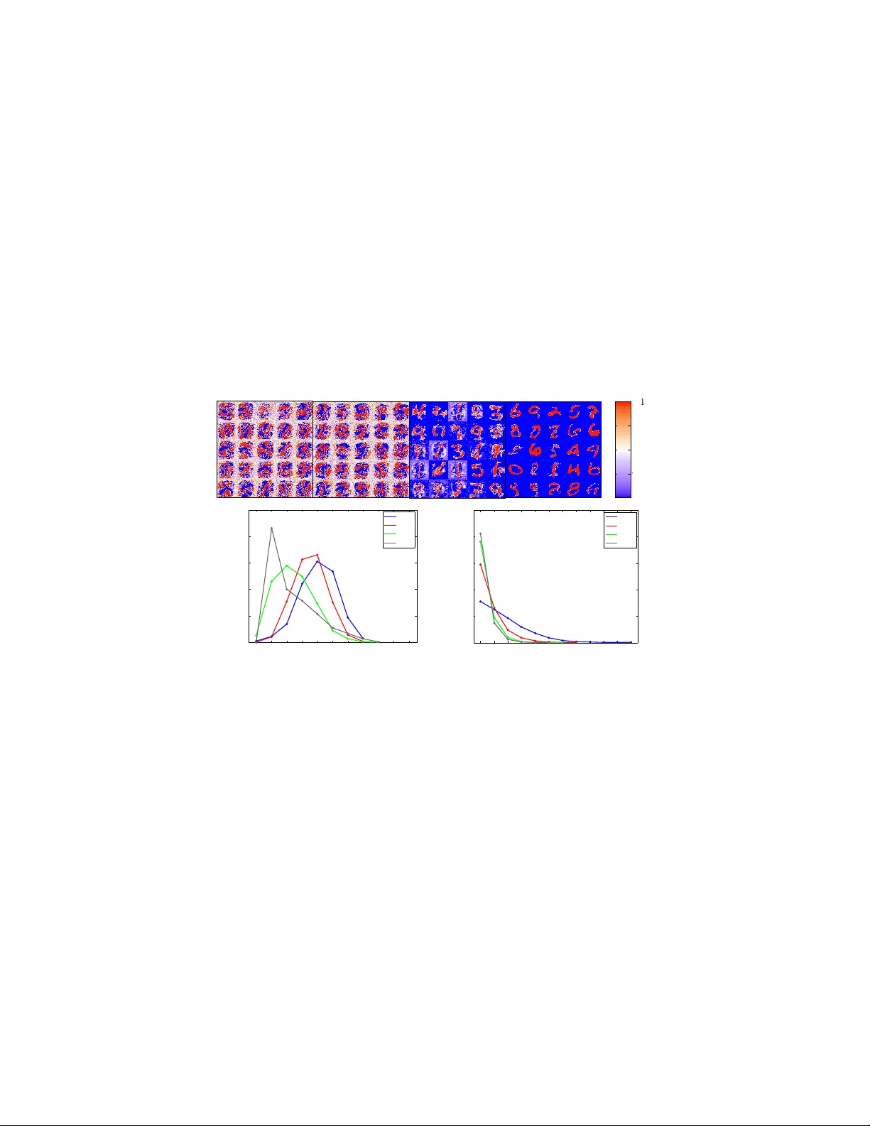
Dense Associativ e Memory f or P attern Recognition Dmitry Kroto v Simons Center for Systems Biology Institute for Advanced Study Princeton, USA krotov@ias.edu John J . Hopfield Princeton Neuroscience Institute Princeton Univ ersity Princeton, USA hopfield@princeton.edu Abstract A model of associati ve memory is studied, which stores and reliably retrie ves many more patterns than the number of neurons in the network. W e propose a simple duality between this dense associativ e memory and neural networks commonly used in deep learning. On the associati ve memory side of this duality , a family of models that smoothly interpolates between two limiting cases can be constructed. One limit is referred to as the feature-matching mode of pattern recognition, and the other one as the prototype re gime. On the deep learning side of the duality , this family corresponds to feedforward neural networks with one hidden layer and various activ ation functions, which transmit the activities of the visible neurons to the hidden layer . This family of activ ation functions includes logistics, rectified linear units, and rectified polynomials of higher degrees. The proposed duality makes it possible to apply energy-based intuition from associative memory to analyze computational properties of neural networks with unusual acti v ation functions – the higher rectified polynomials which until no w hav e not been used in deep learning. The utility of the dense memories is illustrated for two test cases: the logical gate XOR and the recognition of handwritten digits from the MNIST data set. 1 Introduction Pattern recognition and models of associative memory [ 1 ] are closely related. Consider image classification as an example of pattern recognition. In this problem, the network is presented with an image and the task is to label the image. In the case of associativ e memory the network stores a set of memory vectors. In a typical query the network is presented with an incomplete pattern resembling, but not identical to, one of the stored memories and the task is to recov er the full memory . Pixel intensities of the image can be combined together with the label of that image into one vector [ 2 ], which will serve as a memory for the associati ve memory . Then the image itself can be thought of as a partial memory cue. The task of identifying an appropriate label is a subpart of the associati v e memory reconstruction. There is a limitation in using this idea to do pattern recognition. The standard model of associative memory works well in the limit when the number of stored patterns is much smaller than the number of neurons [ 1 ], or equi valently the number of pixels in an image. In order to do pattern recognition with small error rate one would need to store many more memories than the typical number of pixels in the presented images. This is a serious problem. It can be solved by modifying the standard energy function of associativ e memory , quadratic in interactions between the neurons, by including in it higher order interactions. By properly designing the energy function (or Hamiltonian) for these models with higher order interactions one can store and reliably retriev e many more memories than the number of neurons in the network. Deep neural networks ha ve pro ven to be useful for a broad range of problems in machine learning including image classification, speech recognition, object detection, etc. These models are composed of sev eral layers of neurons, so that the output of one layer serves as the input to the next layer . Each 30th Conference on Neural Information Processing Systems (NIPS 2016), Barcelona, Spain. neuron calculates a weighted sum of the inputs and passes the result through a non-linear activ ation function. T raditionally , deep neural networks used acti v ation functions such as hyperbolic tangents or logistics. Learning the weights in such networks, using a backpropagation algorithm, f aced serious problems in the 1980s and 1990s. These issues were largely resolved by introducing unsupervised pre-training, which made it possible to initialize the weights in such a way that the subsequent backpropagation could only gently mov e boundaries between the classes without destroying the feature detectors [ 3 , 4 ]. More recently , it was realized that the use of rectified linear units (ReLU) instead of the logistic functions speeds up learning and improv es generalization [ 5 , 6 , 7 ]. Rectified linear functions are usually interpreted as firing rates of biological neurons. These rates are equal to zero if the input is below a certain threshold and linearly grow with the input if it is above the threshold. T o mimic biology the output should be small or zero if the input is belo w the t hreshold, but it is much less clear what the beha vior of the acti vation function should be for inputs exceeding the threshold. Should it grow linearly , sub-linearly , or faster than linearly? How does this choice af fect the computational properties of the neural network? Are there other functions that would work e ven better than the rectified linear units? These questions to the best of our knowledge remain open. This paper examines these questions through the lens of associativ e memory . W e start by discussing a family of models of associativ e memory with large capacity . These models use higher order (higher than quadratic) interactions between the neurons in the energy function. The associativ e memory description is then mapped onto a neural network with one hidden layer and an unusual acti v ation function, related to the Hamiltonian. W e show that by varying the po wer of interaction vertex in the energy function (or equi v alently by changing the acti v ation function of the neural network) one can force the model to learn representations of the data either in terms of features or in terms of prototypes. 2 Associative memory with lar ge capacity The standard model of associati v e memory [ 1 ] uses a system of N binary neurons, with v alues ± 1 . A configuration of all the neurons is denoted by a vector σ i . The model stores K memories, denoted by ξ µ i , which for the moment are also assumed to be binary . The model is defined by an energy function, which is giv en by E = − 1 2 N X i,j =1 σ i T ij σ j , T ij = K X µ =1 ξ µ i ξ µ j , (1) and a dynamical update rule that decreases the energy at e very update. The basic problem is the following: when presented with a new pattern the network should respond with a stored memory which most closely resembles the input. There has been a large amount of work in the community of statistical physicists inv estigating the capacity of this model, which is the maximal number of memories that the network can store and reliably retrie ve. It has been demonstrated [ 1 , 8 , 9 ] that in case of random memories this maximal value is of the order of K max ≈ 0 . 14 N . If one tries to store more patterns, se veral neighboring memories in the configuration space will merge together producing a ground state of the Hamiltonian (1), which has nothing to do with any of the stored memories. By modifying the Hamiltonian (1) in a way that remo ves second order correlations between the stored memories, it is possible [10] to improv e the capacity to K max = N . The mathematical reason why the model (1) gets confused when many memories are stored is that se veral memories produce contrib utions to the ener gy which are of the same order . In other words the energy decreases too slo wly as the pattern approaches a memory in the configuration space. In order to take care of this problem, consider a modification of the standard ener gy E = − K X µ =1 F  ξ µ i σ i  (2) In this formula F ( x ) is some smooth function (summation ov er index i is assumed). The compu- tational capabilities of the model will be illustrated for two cases. First, when F ( x ) = x n ( n is an integer number), which is referred to as a polynomial ener gy function. Second, when F ( x ) is a 2 rectified polynomial energy function F ( x ) =  x n , x ≥ 0 0 , x < 0 (3) In the case of the polynomial function with n = 2 the network reduces to the standard model of associati ve memory [ 1 ]. If n > 2 each term in (2) becomes sharper compared to the n = 2 case, thus more memories can be packed into the same configuration space before cross-talk intervenes. Having defined the energy function one can deri v e an iterativ e update rule that leads to decrease of the energy . W e use asynchronous updates flipping one unit at a time. The update rule is: σ ( t +1) i = S ig n  K X µ =1  F  ξ µ i + X j 6 = i ξ µ j σ ( t ) j  − F  − ξ µ i + X j 6 = i ξ µ j σ ( t ) j   , (4) The argument of the sign function is the dif ference of two ener gies. One, for the configuration with all but the i -th units clumped to their current states and the i -th unit in the “of f ” state. The other one for a similar configuration, b ut with the i -th unit in the “on” state. This rule means that the system updates a unit, gi ven the states of the rest of the network, in such a w ay that the energy of the entire configuration decreases. For the case of polynomial energy function a very similar family of models was considered in [ 11 , 12 , 13 , 14 , 15 , 16 ]. The update rule in those models was based on the induced magnetic fields, howe v er , and not on the difference of ener gies. The two are slightly dif ferent due to the presence of self-coupling terms. Throughout this paper we use energy-based update rules. Ho w many memories can model (4) store and reliably retrie ve? Consider the case of random patterns, so that each element of the memories is equal to ± 1 with equal probability . Imagine that the system is initialized in a state equal to one of the memories (pattern number µ ). One can deriv e a stability criterion, i.e. the upper bound on the number of memories such that the network stays in that initial state. Define the energy difference between the initial state and the state with spin i flipped ∆ E = K X ν =1  ξ ν i ξ µ i + X j 6 = i ξ ν j ξ µ j  n − K X ν =1  − ξ ν i ξ µ i + X j 6 = i ξ ν j ξ µ j  n , where the polynomial ener gy function is used. This quantity has a mean h ∆ E i = N n − ( N − 2) n ≈ 2 nN n − 1 , which comes from the term with ν = µ , and a variance (in the limit of large N ) Σ 2 = Ω n ( K − 1) N n − 1 , where Ω n = 4 n 2 (2 n − 3)!! The i -th bit becomes unstable when the magnitude of the fluctuation e xceeds the energy g ap h ∆ E i and the sign of the fluctuation is opposite to the sign of the energy gap. Thus the probability that the state of a single neuron is unstable (in the limit when both N and K are large, so that the noise is effecti v ely gaussian) is equal to P error = ∞ Z h ∆ E i dx √ 2 π Σ 2 e − x 2 2Σ 2 ≈ r (2 n − 3)!! 2 π K N n − 1 e − N n − 1 2 K (2 n − 3)!! Requiring that this probability is less than a small v alue, say 0 . 5% , one can find the upper limit on the number of patterns that the network can store K max = α n N n − 1 , (5) where α n is a numerical constant, which depends on the (arbitrary) threshold 0 . 5% . The case n = 2 corresponds to the standard model of associativ e memory and giv es the well known result K = 0 . 14 N . For the perfect reco very of a memory ( P error < 1 / N ) one obtains K max no errors ≈ 1 2(2 n − 3)!! N n − 1 ln( N ) (6) For higher po wers n the capacity rapidly gro ws with N in a non-linear way , allowing the netw ork to store and reliably retrie ve man y more patterns than the number of neurons that it has, in accord 1 with [ 13 , 14 , 15 , 16 ]. This non-linear scaling relationship between the capacity and the size of the network is the phenomenon that we exploit. 1 The n -dependent coefficient in (6) depends on the exact form of the Hamiltonian and the update rule. References [ 13 , 14 , 15 ] do not allow repeated indices in the products over neurons in the energy function, therefore obtain a dif ferent coefficient. In [ 16 ] the Hamiltonian coincides with ours, but the update rule is different, which, ho we ver , results in e xactly the same coefficient as in (6). 3 W e study a family of models of this kind as a function of n . At small n many terms contrib ute to the sum ov er µ in (2) approximately equally . In the limit n → ∞ the dominant contribution to the sum comes from a single memory , which has the largest o verlap with the input. It turns out that optimal computation occurs in the intermediate range. 3 The case of XOR The case of XOR is elementary , yet instructi v e. It is presented here for three reasons. First, it illustrates the construction (2) in this simplest case. Second, it shows that as n increases, the computational capabilities of the network also increase. Third, it provides the simplest example of a situation in which the number of memories is larger than the number of neurons, yet the network w orks reliably . The problem is the following: given tw o inputs x and y produce an output z such that the truth table x y z -1 -1 -1 -1 1 1 1 -1 1 1 1 -1 is satisfied. W e will treat this task as an associativ e memory problem and will simply embed the four examples of the input-output triplets x, y, z in the memory . Therefore the network has N = 3 identical units: two of which will be used for the inputs and one for the output, and K = 4 memories ξ µ i , which are the four lines of the truth table. Thus, the energy (2) is equal to E n ( x, y, z ) = −  − x − y − z  n −  − x + y + z  n −  x − y + z  n −  x + y − z  n , (7) where the energy function is chosen to be a polynomial of de gree n . For odd n , energy (7) is an odd function of each of its ar guments, E n ( x, y, − z ) = − E n ( x, y, z ) . For ev en n , it is an e ven function. For n = 1 it is equal to zero. Thus, if e valuated on the corners of the cube x, y, z = ± 1 , it reduces to E n ( x, y, z ) =    0 , n = 1 C n , n = 2 , 4 , 6 , ... C n xy z , n = 3 , 5 , 7 , ..., (8) where coefficients C n denote numerical constants. In order to solve the XOR problem one can present to the network an “incomplete pattern” of inputs ( x, y ) and let the output z adjust to minimize the ener gy of the three-spin configuration, while holding the inputs fixed. The network clearly cannot solv e this problem for n = 1 and n = 2 , since the ener gy does not depend on the spin configuration. The case n = 2 is the standard model of associativ e memory . It can also be thought of as a linear perceptron, and the inability to solve this problem represents the well known statement [ 17 ] that linear perceptrons cannot compute XOR without hidden neurons. The case of odd n ≥ 3 provides an interesting solution. Given tw o inputs, x and y , one can choose the output z that minimizes the energy . This leads to the update rule z = S ig n  E n ( x, y, − 1) − E n ( x, y, +1)  = S ig n  − xy  Thus, in this simple case the network is capable of solving the problem for higher odd v alues of n , while it cannot do so for n = 1 and n = 2 . In case of rectified polynomials, a similar construction solves the problem for an y n ≥ 2 . The network works well in spite of the fact that K > N . 4 An example of a pattern r ecognition pr oblem, the case of MNIST The MNIST data set is a collection of handwritten digits, which has 60000 training examples and 10000 test images. The goal is to classify the digits into 10 classes. The visible neurons, one for each pixel, are combined together with 10 classification neurons in one vector that defines the state of the network. The visible part of this vector is treated as an “incomplete” pattern and the associativ e memory is allowed to calculate a completion of that pattern, which is the label of the image. Dense associativ e memory (2) is a recurrent network in which every neuron can be updated multiple times. For the purposes of digit classification, ho wev er , this model will be used in a very limited 4 capacity , allowing it to perform only one update of the classification neurons. The network is initialized in the state when the visible units v i are clamped to the intensities of a gi ven image and the classification neurons are in the of f state x α = − 1 (see Fig.1A). The network is allowed to make one update of the classification neurons, while keeping the visible units clamped, to produce the output c α . The update rule is similar to (4) except that the sign is replaced by the continuous function g ( x ) = tanh( x ) c α = g  β K X µ =1  F  − ξ µ α x α + X γ 6 = α ξ µ γ x γ + N X i =1 ξ µ i v i  − F  ξ µ α x α + X γ 6 = α ξ µ γ x γ + N X i =1 ξ µ i v i   , (9) where parameter β regulates the slope of g ( x ) . The proposed digit class is giv en by the number of a classification neuron producing the maximal output. Throughout this section the rectified polynomials (3) are used as functions F . T o learn effecti v e memories for use in pattern classification, an objectiv e function is defined (see Appendix A in Supplemental), which penalizes the discrepancy A B v i c ↵ v i x ↵ 0 500 1000 1500 2000 2500 3000 1.4 1.5 1.6 1.7 1.8 1.9 2 error, test set Epochs number of epochs number of epochs test error, % test error, % 0 500 1000 1500 2000 2500 3000 1.4 1.5 1.6 1.7 1.8 1.9 2 error, test set Epochs 158-262 epochs n =3 n =2 179-312 epochs Figure 1: (A) The network has N = 28 × 28 = 784 visible neurons and N c = 10 classification neurons. The visible units are clamped to intensities of pixels (which is mapped on the segment [ − 1 , 1] ), while the classification neurons are initialized in the state x α and then updated once to the state c α . (B) Behavior of the error on the test set as training progresses. Each curve corresponds to a dif ferent combination of hyperparameters from the optimal window , which was determined on the validation set. The arrows sho w the first time when the error falls belo w a 2% threshold. All models hav e K = 2000 memories (hidden units). between the output c α and the target output. This objectiv e function is then minimized using a backpropagation algorithm. The learning starts with random memories drawn from a Gaussian distribution. The backpropagation algorithm then finds a collection of K memories ξ µ i,α , which minimize the classification error on the training set. The memories are normalized to stay within the − 1 ≤ ξ µ i,α ≤ 1 range, absorbing their ov erall scale into the definition of the parameter β . The performance of the proposed classification frame work is studied as a function of the po wer n . The next section shows that a rectified polynomial of po wer n in the ener gy function is equi valent to the rectified polynomial of po wer n − 1 used as an activation function in a feedforward neural network with one hidden layer of neurons. Currently , the most common choice of acti v ation functions for training deep neural networks is the ReLU, which in our language corresponds to n = 2 for the energy function. Although not currently used to train deep networks, the case n = 3 would correspond to a rectified parabola as an activ ation function. W e start by comparing the performances of the dense memories in these two cases. The performance of the network depends on n and on the remaining hyperparameters, thus the hyper- parameters should be optimized for each v alue of n . In order to test the variability of performances for v arious choices of hyperparameters at a giv en n , a window of hyperparameters for which the network works well on the validation set (see the Appendix A in Supplemental) was determined. Then many netw orks were trained for v arious choices of the hyperparameters from this windo w to ev aluate the performance on the test set. The test errors as training progresses are sho wn in Fig.1B. While there is substantial v ariability among these samples, on av erage the cluster of trajectories for n = 3 achiev es better results on the test set than that for n = 2 . These error rates should be compared with error rates for backpropagation alone without the use of generati v e pretraining, v arious kinds of regularizations (for e xample dropout) or adv ersarial training, all of which could be added to our construction if necessary . In this class of models the best published results are all 2 in the 1 . 6% range [ 18 ], see also controls in [ 19 , 20 ]. This agrees with our results for n = 2 . The n = 3 case does slightly better than that as is clear from Fig.1B, with all the samples performing better than 1 . 6% . 2 Although there are better results on pixel permutation in v ariant task, see for example [19, 20, 21, 22]. 5 Higher rectified polynomials are also f aster in training compared to ReLU. F or the n = 2 case, the error crosses the 2% threshold for the first time during training in the range of 179-312 epochs. For the n = 3 case, this happens earlier on average, between 158-262 epochs. For higher powers n this speed-up is larger . This is not a huge effect for a small dataset such as MNIST . Howe ver , this speed-up might be v ery helpful for training lar ge networks on lar ge datasets, such as ImageNet. A similar effect was reported earlier for the transition between saturating units, such as logistics or hyperbolic tangents, to ReLU [ 7 ]. In our family of models that result corresponds to mo ving from n = 1 to n = 2 . Featur e to pr ototype transition How does the computation performed by the neural network change as n varies? There are two extreme classes of theories of pattern recognition: feature-matching and formation of a prototype. According to the former , an input is decomposed into a set of features, which are compared with those stored in the memory . The subset of the stored features activ ated by the presented input is then interpreted as an object. One object has many features; features can also appear in more than one object. The prototype theory provides an alternativ e approach, in which objects are recognized as a whole. The prototypes do not necessarily match the object exactly , but rather are blurred abstract 64 128 192 256 64 128 192 256 64 128 192 256 64 128 192 256 0 1 2 3 4 5 6 7 8 9 10 0 10 20 30 40 50 percent of active memories number of strongly positively driven RU n=2 n=3 n=20 n=30 1 2 3 4 5 6 7 8 9 10 11 12 0 2000 4000 6000 8000 10000 number of test images number of memories strongly contributing to the correct RU n=2 n=3 n=20 n=30 64 128 192 256 number of RU with ⇠ µ ↵ > 0 . 99 number of memories making the decision percent of memories, % number of test images  1  0 . 5 0 . 5 0 1 n =2 n =3 n = 20 n = 30 error test =1 . 51% error test =1 . 44% error test =1 . 61% error test =1 . 80% Figure 2: W e show 25 randomly selected memories (feature detectors) for four networks, which use recti- fied polynomials of degrees n = 2 , 3 , 20 , 30 as the energy function. The magnitude of a memory element corresponding to each pixel is plotted in the location of that pixel, the color bar explains the color code. The histograms at the bottom are explained in the text. The error rates refer to the particular four samples used in this figure. RU stands for recognition unit. representations which include all the features that an object has. W e argue that the computational models proposed here describe feature-matching mode of pattern recognition for small n and the prototype regime for large n . This can be anticipated from the sharpness of contrib utions that each memory makes to the total energy (2). For large n the function F ( x ) peaks much more sharply around each memory compared to the case of small n . Thus, at large n all the information about a digit must be written in only one memory , while at small n this information can be distributed among sev eral memories. In the case of intermediate n some learned memories beha ve like features while others behav e like prototypes. These two classes of memories work together to model the data in an efficient w ay . The feature to prototype transition is clearly seen in memories shown in Fig.2. For n = 2 or 3 each memory does not look lik e a digit, b ut resembles a pattern of acti vity that might be useful for recognizing se veral dif ferent digits. For n = 20 many of the memories can be recognized as digits, which are surrounded by white mar gins representing elements of memories having approximately zero values. These margins describe the variability of thicknesses of lines of different training examples and mathematically mean that the ener gy (2) does not depend on whether the corresponding pixel is on or off. For n = 30 most of the memories represent prototypes of whole digits or large portions of digits, with a small admixture of feature memories that do not resemble any digit. 6 The feature to prototype transition can be visualized by sho wing the feature detectors in situations when there is a natural ordering of pixels. Such ordering e xists in images, for e xample. In general situations, ho wev er , there is no preferred permutation of visible neurons that would reveal this structure ( e.g . in the case of genomic data). It is therefore useful to develop a measure that permits a distinction to be made between features and prototypes in the absence of such visual space. T owards the end of training most of the recognition connections ξ µ α are approximately equal to ± 1 . One can choose an arbitrary cutoff, and count the number of recognition connections that are in the “on” state ( ξ µ α = +1 ) for each memory . The distribution function of this number is sho wn on the left histogram in Fig.2. Intuitiv ely , this quantity corresponds to the number of different digit classes that a particular memory votes for . At small n , most of the memories vote for three to fiv e dif ferent digit classes, a behavior characteristic of features. As n increases, each memory specializes and votes for only a single class. In the case n = 30 , for example, more than 40% of memories vote for only one class, a behavior characteristic of prototypes. A second way to see the feature to prototype transition is to look at the number of memories which mak e large contrib utions to the classification decision (right histogram in Fig.2). For each test image one can find the memory that makes the largest contrib ution to the ener gy gap, which is the sum ov er µ in (9). Then one can count the number of memories that contribute to the gap by more than 0.9 of this largest contribution. For small n , there are many memories that satisfy this criterion and the distribution function has a long tail. In this regime se veral memories are cooperating with each other to make a classification decision. For n = 30 , ho wev er , more than 8000 of 10000 test images do not ha ve a single other memory that w ould make a contrib ution comparable with the largest one. This result is not sensiti ve to the arbitrary choice ( 0 . 9 ) of the cutoff. Interestingly , the performance remains competitiv e ev en for very large n ≈ 20 (see Fig.2) in spite of the fact that these networks are doing a very dif ferent kind of computation compared with that at small n . 5 Relationship to a neural network with one hidden layer In this section we deri ve a simple duality between the dense associati v e memory and a feedforward neural network with one layer of hidden neurons. In other words, we show that the same computational model has two v ery dif ferent descriptions: one in terms of associati ve memory , the other one in terms v i c ↵ v i v i c ↵ f g h µ x ↵ =  " Figure 3: On the left a feedforward neural network with one layer of hidden neurons. The states of the visible units are transformed to the hidden neurons using a non-linear function f , the states of the hidden units are transformed to the output layer using a non-linear function g . On the right the model of dense associativ e memory with one step update (9). The two models are equiv alent. of a network with one layer of hidden units. Using this correspondence one can transform the family of dense memories, constructed for dif ferent v alues of po wer n , to the language of models used in deep learning. The resulting neural networks are guaranteed to inherit computational properties of the dense memories such as the feature to prototype transition. The construction is v ery similar to (9), except that the classification neurons are initialized in the state when all of them are equal to − ε , see Fig.3. In the limit ε → 0 one can expand the function F in (9) so that the dominant contribution comes from the term linear in ε . Then c α ≈ g h β K X µ =1 F 0  N X i =1 ξ µ i v i  ( − 2 ξ µ α x α ) i = g h K X µ =1 ξ µ α F 0  ξ µ i v i  i = g h K X µ =1 ξ µ α f  ξ µ i v i  i , (10) where the parameter β is set to β = 1 / (2 ε ) (summation ov er the visible inde x i is assumed). Thus, the model of associati ve memory with one step update is equi v alent to a con ventional feedforward neural network with one hidden layer pro vided that the activ ation function from the visible layer to the hidden layer is equal to the deriv ati ve of the ener gy function f ( x ) = F 0 ( x ) (11) 7 The visible part of each memory serves as an incoming weight to the hidden layer , and the recognition part of the memory serves as an outgoing weight from the hidden layer . The expansion used in (10) is justified by a condition N P i =1 ξ µ i v i  N c P α =1 ξ µ α x α , which is satisfied for most common problems, and is simply a statement that labels contain far less information than the data itself. From the point of view of associativ e memory , the dominant contribution shaping the basins of attraction comes from the low energy states. Therefore mathematically it is determined by the asymptotics of the activ ation function f ( x ) , or the energy function F ( x ) , at x → ∞ . Thus different acti vation functions ha ving similar asymptotics at x → ∞ should fall into the same universality class and should hav e similar computational properties. In the table below we list some common activ ation activation function energy function n f ( x ) = tanh( x ) F ( x ) = ln  cosh( x )  ≈ x , at x → ∞ 1 f ( x ) = logistic function F ( x ) = ln  1 + e x  ≈ x , at x → ∞ 1 f ( x ) = ReLU F ( x ) ∼ x 2 , at x → ∞ 2 f ( x ) = ReP n − 1 F ( x ) = ReP n n functions used in models of deep learning, their associati ve memory counterparts and the po wer n which determines the asymptotic behavior of the ener gy function at x → ∞ .The results of section 4 suggest that for not too large n the speed of learning should improv e as n increases. This is consistent with the previous observ ation that ReLU are faster in training than hyperbolic tangents and logistics [ 5 , 6 , 7 ]. The last row of the table corresponds to rectified polynomials of higher degrees. T o the best of our knowledge these acti v ation functions hav e not been used in neural networks. Our results suggest that for some problems these higher power activ ation functions should hav e ev en better computational properties than the rectified liner units. 6 Discussion and conclusions What is the relationship between the capacity of the dense associati ve memory , calculated in section 2, and the neural network with one step update that is used for digit classification? Consider the limit of very large β in (9), so that the hyperbolic tangent is approximately equal to the sign function, as in (4). In the limit of suf ficiently lar ge n the network is operating in the prototype re gime. The presented image places the initial state of the network close to a local minimum of ener gy , which corresponds to one of the prototypes. In most cases the one step update of the classification neurons is sufficient to bring this initial state to the nearest local minimum, thus completing the memory recovery . This is true, ho wev er , only if the stored patterns are stable and ha ve basins of attraction around them of at least the size of one neuron flip, which is exactly (in the case of random patterns) the condition giv en by (6). For correlated patterns the maximal number of stored memories might be dif ferent from (6), ho wev er it still rapidly increases with increase of n . The associati ve memory with one step update (or the feedforward neural netw ork) is exactly equi v alent to the full associati ve memory with multiple updates in this limit. The calculation with random patterns thus theoretically justifies the expectation of a good performance in the prototype regime. T o summarize, this paper contains three main results. First, it is shown how to use the general framew ork of associativ e memory for pattern recognition. Second, a family of models is constructed that can learn representations of the data in terms of features or in terms of prototypes, and that smoothly interpolates between these two extreme regimes by v arying the power of interaction vertex. Third, there exists a simple duality between a one step update version of the associati ve memory model and a feedforward neural network with one layer of hidden units and an unusual activ ation function. This duality makes it possible to propose a class of activ ation functions that encourages the network to learn representations of the data with v arious proportions of features and prototypes. These activ ation functions can be used in models of deep learning and should be more effecti ve than the standard choices. They allow the networks to train faster . W e have also observ ed an improvement of generalization ability in networks trained with the rectified parabola activ ation function compared to the ReLU for the case of MNIST . While these ideas were illustrated using the simplest architecture of the neural network with one layer of hidden units, the proposed acti vation functions can also be used in multilayer architectures. W e did not study various regularizations (weight decay , dropout, etc), which can be added to our construction. The performance of the model supplemented with these regularizations, as well as performance on other common benchmarks, will be reported else where. 8 A ppendix A. Details of experiments with MNIST . The networks were trained using stochastic gradient descent with minibatches of a relati vely lar ge size, 100 digits of each class, 1000 digits in total. Training was done for 3000 epochs. Initial weights were generated from a Gaussian distrib ution N ( − 0 . 3 , 0 . 3) . Momentum ( 0 . 6 ≤ p ≤ 0 . 95 ) was used to smooth out oscillations of gradients coming from the indi vidual minibatches. The learning rate was decreasing with time according to ε ( t ) = ε 0 f t , f = 0 . 998 , (12) where t is the number of epoch. T ypical values are 0 . 01 ≤ ε 0 ≤ 0 . 04 . The weights (memories) were updated after each minibatch according to V µ I ( t ) = pV µ I ( t − 1) − ∂ ξ µ I C ξ µ I ( t ) = ξ µ I ( t − 1) + ε V µ I ( t ) max J | V µ J ( t ) | , (13) where t is the number of update, I = ( i, α ) is an index which unites the visible and the classification units. The proposed update in (13) is normalized so that the largest update of the weights for each hidden unit (memory) is equal to ε . This normalization is equiv alent to using different learning rates for each indi vidual memory . It prevents the network from getting stuck on a plateau. All weights were constrained to stay within the − 1 ≤ ξ µ I ≤ 1 range. Therefore, if after an update some weights exceeded 1 , they were truncated to make them equal to 1 (and similarly for − 1 ). The slope of the function g ( x ) in (9) is controlled by the effecti ve temperature β = 1 /T n , which is measured in “neurons” or “pixels”. For large n the temperature can be kept constant throughout the entire training ( 500 ≤ T ≤ 700 ). For small n we found useful to start at a high temperature T i , and then linearly decrease it to the final value T f during the first 200 epochs ( 250 ≤ T i ≤ 400 , 30 ≤ T f ≤ 100 ). The temperature stays constant after that. All the models have K = 2000 memories (hidden units). The MNIST dataset contains 60000 training e xamples, which were randomly split into 50000 training cases and 10000 v alidation cases. For each hyperparameter a windo w of v alues was selected, such that the error on the v alidation set after 3000 epochs is less than a certain threshold. After that the entire set of 60000 examples was used to train the network (for 3000 epochs) for v arious v alues of the hyperparameters from this optimal windo w to ev aluate the performance on the test set. The v alidation set was not used for early stopping. The objectiv e function is gi ven by C = X training examples N c X α =1  c α − t α  2 m , (14) where t α is the target output ( t α = − 1 for the wrong classes and t α = +1 for the correct class). The case m = 1 corresponds to the standard quadratic error . For large powers m the function x 2 m is small for | x | < 1 and rapidly gro ws for | x | > 1 . Therefore, higher values of m emphasize training examples which produce largest discrepanc y with the target output more strongly compared to those examples which are already sufficiently close to the target output. Such emphasis encourages the network to concentrate on correcting mistakes and mo ving the decision boundary farther a way from the barely correct examples rather than on fitting better and better the training examples which hav e already been easily and correctly classified. Although much of what we discuss is valid for arbitrary value of m , including m = 1 , we found that higher values of m reduce overfitting and improve generalization at least in the limit of large n . For small n , we used m = 2 , 3 , 4 . For n = 20 , 30 , larger v alues of m ≈ 30 worked better . W e also tried cross-entropy objectiv e function together with softmax output units. The results were worse and are not presented here. The training can be done both in the associativ e memory description and in the neural network description. The two are related by the duality of section 5. Below we gi ve the explicit e xpressions for the update rule (13) for these two methods. Consider a minibatch of size M . In the associativ e memory framework one can define two ( N + N c ) × M N c matrices U αA J and V αA J (index A = 1 ...M runs over the training examples of the 9 minibatch, greek indices α, γ = 1 ...N c run over classification neurons, index i = 1 ...N runs over visible neurons, indices I , J = 1 ... ( N + N c ) unite all the neurons, visible and classification). U αA i = v A i V αA i = v A i U αA γ = − 1 V αA γ =  +1 , α = γ − 1 , α 6 = γ The update rule (9) can then be rewritten as c A α = g h β  K X µ =1 F n ( ξ µ J V αA J ) − F n ( ξ µ J U αA J ) i , where F n ( x ) is the rectified polynomial of po wer n , and summation o ver inde x J is assumed. The deriv ati ve of the objecti v e function (14) is giv en by ∂ ξ µ I C = (2 mβ n ) M X A =1 N c X α =1  c A α − t A α  2 m − 1 h 1 −  c A α  2 ih F n − 1 ( ξ µ J V αA J ) V αA I − F n − 1 ( ξ µ J U αA J ) U αA I i The indices A and α can be united in one tensor product inde x, so that the two sums can be ef ficiently calculated using matrix-matrix multiplication. While this w ay of training the netw ork is most closely related to the theoretical calculations presented in the main text, it is computationally inef ficient. The second dimension of the matrices U and V is N c times larger than the size of the minibatch. This can become problematic if the classification problem in v olves man y classes. For this reason it is computationally easier to train the dense memory in the dual description, which is more closely related to the con ventional methods used in deep learning. In this framework, the minibatch matrix v A i has N × M elements. The update rule is c A α = g h β K X µ =1 ξ µ α f n ( ξ µ i v A i ) i , where f n ( x ) is a rectified polynomial of po wer 3 n , and summation ov er the visible index i = 1 ...N is assumed. The deriv ativ es of the objectiv e function (14) are gi ven by ∂ ξ µ i C = (2 mβ n ) M X A =1 N c X α =1  c A α − t A α  2 m − 1 h 1 −  c A α  2 i ξ µ α f n − 1  ξ µ j v A j  v A i ∂ ξ µ α C = (2 mβ ) M X A =1  c A α − t A α  2 m − 1 h 1 −  c A α  2 i f n  ξ µ j v A j  , where summation ov er the visible index j is assumed. These expressions are very similar to the con ventional deriv ati ves used in networks with rectified linear acti vation functions, but they use power acti v ation functions instead. The minibatch training can be efficiently implemented on GPU. A ppendix B. Capacity of Dense associative memory . In section 2 of the main text a theoretical calculation of the capacity for model (4) was presented in the case of po wer ener gy functions. In section 5 an intuitiv e argument (based on the lo w energy states of the Hamiltonian) was given arguing that the capacities of the models with power energy functions and rectified polynomial energy functions should be very similar . In this appendix we compare the theoretical results of section 2 with numerical simulations and numerically validate the intuitiv e argument about lo w ener gy states. A random set of K = 2000 binary memory vectors was generated in the model with N = 100 neurons. A collection of 10000 random initial configurations of binary spins were evolv ed according to (4) until conv ergence. The quality of memory recovery was measured by the overlap between 3 One should remember that the energy function of power n is dual to the activ ation function of power n − 1 . Here, for the sake of notations, we describe the training procedure for general n . 10 the final configuration of spins  σ i = σ ( t →∞ ) i  and the closest memory , max µ  N P i =1 ξ µ i σ i  . If the recov ery is perfect, this quantity is equal to N ; if some of the spins failed to match a memory vector , this quantity is smaller than N . In Fig. 4 the histograms of the ov erlaps are shown for n = 2 , 3 , 4 in case of po wer and rectified polynomial ener gy functions. For n = 2 , 3 the number of memories ( K = 2000 ) places the model above the capacity (according to (6), K max no errors ≈ 11 for n = 2 and K max no errors ≈ 360 for n = 3 ). Thus, the model is unable to reconstract the memories. For n = 4 , the number of memories is below the capacity ( K max no errors ≈ 7240 ), thus the distribution sharply peaks at perfect recov ery . For n ≥ 5 all 10000 samples con ver ge to one of the memories. Qualitatively , this behavior is demonstrated by both po wer models and rectified models. 0 20 40 60 80 100 0 20 40 60 80 100 maximal overlap percent of trials n=2 n=3 n=4 N = 100 K = 2000 maximal overlap max µ ( ⇠ µ i  i ) percent of trials 0 20 40 60 80 100 0 20 40 60 80 100 maximal overlap percent of trials n=2 n=3 n=4 percent of trials maximal overlap max µ ( ⇠ µ i  i ) N = 100 K = 2000 F ( x )= ( x n ,x  0 0 ,x < 0 F ( x )= x n Figure 4: The histograms of overlaps for models with n = 2 , 3 , 4 with power energy functions (left) and rectified polynomial energy functions (right). Each histogram has 10000 samples in it. A family of models with 50 ≤ N ≤ 200 and 50 ≤ K ≤ 1500 was studied. For each combination of N and K a set of binary memory vectors was generated to make a model of associativ e memory . After that 1000 random binary initial conditions were ev olved according to (4) until con v ergence. K 1 / 2 is the number of memories when half (500) of these samples perfectly con ver ge to one of the memories. In Fig. 5 the K 1 / 2 dependence of N is shown for the po wer and the rectified models with n = 3 . The solid curve is giv en by Eq.(6). The results of numerical simulations for the case of power activ ation functions are consistent with the theoretical calculation (6). The results for the rectified polynomials are a little bit abov e the theoretical curve, b ut show similar non-linear beha vior . 0 50 100 150 200 0 200 400 600 800 1000 1200 1400 1600 A A A A A A N K 1 / 2 n =3 n =3 rect.p theory Figure 5: Scaling behavior of the capacity vs. the number of neurons for n = 3 with power and rectified polynomial energy functions. Solid curve is the theoretical result (6). 11 Acknowledgments W e thank B. Chazelle, D. Huse, A. Levine, M. Mitchell, R. Monasson, L. Peliti, D. Raskov alo v , B. Xue, and all the members of the Simons Center for Systems Biology at IAS for useful discussions. W e especially thank Y . Roudi for pointing out the reference [ 13 ] to us. The work of DK is supported by Charles L. Brown membership at IAS. References [1] Hopfield, J.J., 1982. Neural networks and physical systems with emergent collectiv e computational abilities. Proceedings of the national academy of sciences, 79(8), pp.2554-2558. [2] LeCun, Y ., Chopra, S., Hadsell, R., Ranzato, M. and Huang, F ., 2006. A tutorial on energy-based learning. Predicting structured data, 1, p.0. [3] Hinton, G.E., Osindero, S. and T eh, Y .W ., 2006. A fast learning algorithm for deep belief nets. Neural computation, 18(7), pp.1527-1554. [4] Hinton, G.E. and Salakhutdinov , R.R., 2006. Reducing the dimensionality of data with neural networks. Science, 313(5786), pp.504-507. [5] Nair , V . and Hinton, G.E., 2010. Rectified linear units improve restricted boltzmann machines. In Proceed- ings of the 27th International Conference on Machine Learning (ICML-10) (pp. 807-814). [6] Glorot, X., Bordes, A. and Bengio, Y ., 2011. Deep sparse rectifier neural networks. In International Conference on Artificial Intelligence and Statistics (pp. 315-323). [7] Krizhevsk y , A., Sutskever , I. and Hinton, G.E., 2012. ImageNet classification with deep conv olutional neural networks. In Adv ances in neural information processing systems (pp. 1097-1105). [8] Amit, D.J., Gutfreund, H. and Sompolinsky , H., 1985. Storing infinite numbers of patterns in a spin-glass model of neural networks. Physical Re view Letters, 55(14), p.1530. [9] McEliece, R.J., Posner, E.C., Rodemich, E.R. and V enkatesh, S.S., 1987. The capacity of the Hopfield associativ e memory . Information Theory , IEEE T ransactions on, 33(4), pp.461-482. [10] Kanter , I. and Sompolinsky , H., 1987. Associative recall of memory without errors. Physical Revie w A, 35(1), p.380. [11] Chen, H.H., Lee, Y .C., Sun, G.Z., Lee, H.Y ., Maxwell, T . and Giles, C.L., 1986. High order correlation model for associativ e memory . In Neural Networks for Computing (V ol. 151, No. 1, pp. 86-99). AIP Publishing. [12] Psaltis, D. and P ark, C.H., 1986. Nonlinear discriminant functions and associati ve memories. In Neural networks for computing (V ol. 151, No. 1, pp. 370-375). AIP Publishing. [13] Baldi, P . and V enkatesh, S.S., 1987. Number of stable points for spin-glasses and neural netw orks of higher orders. Physical Re view Letters, 58(9), p.913. [14] Gardner , E., 1987. Multiconnected neural network models. Journal of Physics A: Mathematical and General, 20(11), p.3453. [15] Abbott, L.F . and Arian, Y ., 1987. Storage capacity of generalized networks. Physical Re view A, 36(10), p.5091. [16] Horn, D. and Usher , M., 1988. Capacities of multiconnected memory models. Journal de Physique, 49(3), pp.389-395. [17] Minsky , M. and Papert, S., 1969. Perceptron: an introduction to computational geometry . The MIT Press, Cambridge, expanded edition, 19(88), p.2. [18] Simard, P .Y ., Steinkraus, D. and Platt, J.C., 2003, August. Best practices for con volutional neural networks applied to visual document analysis. In null (p. 958). IEEE. [19] Sriv asta va, N., Hinton, G., Krizhe vsky , A., Sutskev er , I. and Salakhutdinov , R., 2014. Dropout: A simple way to prev ent neural networks from overfitting. The Journal of Machine Learning Research, 15(1), pp.1929-1958. [20] W an, L., Zeiler , M., Zhang, S., LeCun, Y . and Fergus, R., 2013. Re gularization of neural networks using dropconnect. In Proceedings of the 30th International Conference on Machine Learning (ICML-13) (pp. 1058-1066). [21] Goodfellow , I.J., Shlens, J. and Szegedy , C., 2014. Explaining and harnessing adversarial examples. arXi v preprint [22] Rasmus, A., Berglund, M., Honkala, M., V alpola, H. and Raiko, T ., 2015. Semi-supervised learning with ladder networks. In Adv ances in Neural Information Processing Systems (pp. 3546-3554). 12