Box-Cox symmetric distributions and applications to nutritional data

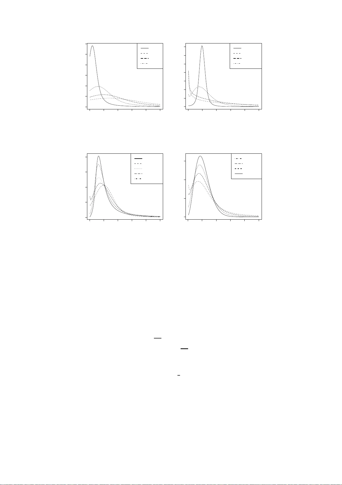
Box-Cox symmetric distributions and applications to nutritional data Silvia L.P . Fe rrari ∗ Department of Statistics, University of S ˜ ao Paulo, S ˜ ao Paulo, Brazil Giovana Fumes Department of Exact Sciences, ESALQ , University of S ˜ ao Paulo, Piracicaba, Brazil Abstract W e i ntroduce and study the Box-Cox s ymmetric class of dist ributions, which is useful for modeling positively skewed, possibly heavy-tailed, data. The new cla ss of distribu- tions includes the Box-Cox t, Bo x -Cox Cole-Green (or Box-Cox normal) , Box-Cox power exponent ial distributions, and the class o f t he log-symmet ric distributions as special cases. It provides easy parameter inte rpretation, which makes i t convenient for r egr es- sion modeling purposes . A d ditionally , it provides e nough flexibility to handle outliers. The us efulness of the Box-Cox symmetric models is illustrated in a series of applica tions to nutritional data. Key words: B ox-Cox transfor mation; Symmetric distributions; Box-Cox p ower exponen- tial distr ibution; Box-Cox slash distribution; Box-Cox t distr ibution; Log -symmetric d is- tributions; Nutrients intake . 1 Introduc tion It is well-known that positive cont inuous data usually present positive skewness and outlier observations. This is the typical situation with survival times, nutrients intake a nd family income data, among many other examples. Since Box and C ox (1964) seminal paper , the Box-Cox power transformatio n has be e n ro utinely employed for transforming to normality . Let Y be a positive random variable. The Box-Cox transfor mation is defined as ( Y λ − 1) /λ, if λ , 0, and log Y , if λ = 0. Despite its popularity and ease of implementation, this approach, however , has drawbacks, one of them being the fact that the model parameters cannot be ∗ Corresponding a uthor . Email: silviaferrari@usp.br 1 easily interpr eted in terms of the original response. A conceptual shortcoming is that the support of the transformed variable is not the whole real line and hence a (non-tr uncated) normal distribution should not be assumed for the transformed data. An alternative appro ach to the Box-Cox transformation that allows the parameters to be interpr etable as characterist ics of the original data is the Box-Cox Cole-Green distribution (or Box-Cox normal distribution) ; see Cole and Gr een (1992 ). It uses the Box-Cox approach, but the parameters are incorporated in to the transformation. The Box-Cox Cole-Gr een distribution has support in R + and is defined from the transformation Z ≡ h ( Y ; µ, σ , λ ) =          1 σλ   Y µ  λ − 1  , if λ , 0 , 1 σ log  Y µ  , if λ = 0 , (1) wher e µ > 0, σ > 0, −∞ < λ < ∞ , assuming that Z has a standard normal distribu- tion truncated at a suitable interval of the real line; details are given in the ne xt section. The Box-Cox symmetric (BCS) class of distributions defined in this paper replaces the nor- mal distribution by the class of the continuous standard symmetric distributio ns. Replac- ing the normal distribution by the Stu dent-t and the power exponential distributions r e- sults in the Box-Cox t (Rigby and Stasinopoulos; 2006) and the Box-Cox power exponential (Rigby and Stasinopoulos; 2004; V o udouris et al.; 2012) distribut ions. Ad d itionally , it gener- alizes the class of the log symmetric distributions (V anegas a nd Paula; 20 1 6, 2015). The paper unfolds as follows. In Sectio n 2, the Box-Cox symmetric class of distribut ions is defined, some properties are stated and interpr etation of the parameters i n terms of quantiles is discussed. T ail he a viness of Box-Cox symmetr ic distribut ions is studied in Section 3. It is shown that the Box-Cox symmetric class of distributions allows much mor e tail flexibility than the log-symmetric distributions. Likelihood-based inference in discussed in Section 4. It is suggested that the choice of the symmetric distribution may lead to robust estimation against outliers. In Section 5, applications to 3 3 nutrients intake da ta are presented, and a comparison of alternative appro aches is provided. Finally , concluding r emarks (Section 6) close the paper . T echnical details are left for the Appe nd ix. 2 Box-Cox symmetr ic distribu tions A continuous random variable W is said to have a symmetric distribut ion with location parameter µ ∈ R , scale parameter σ > 0 and density generating function r , and we write W ∼ S ( µ , σ ; r ), if its probability density function (pdf) is given by f W ( w ) = 1 σ r  w − µ σ  2 ! , w ∈ R , (2) wher e r ( · ) satisfies r ( u ) > 0, for u ≥ 0, a nd R ∞ 0 u − 1 / 2 r ( u )d u = 1. The class of the symmetric distributions has a number of well-known distributions as special cases depending on the 2 choice of r . It includes the normal distribution as well as the Student-t, power exponential, type I logistic, type II logistic and slash distributions among others. Densities in this family have quite di ff erent tail beha viors, a nd some of them may have heavier or lighter tails than the normal distribution. The symmetric distributions have some interest ing pro perties. Some of them follow: (i) If W ∼ S ( µ , σ ; r ), its characteristic function is ψ W ( t ) = e it µ ϕ ( t 2 σ 2 ), t ∈ R , for some function ϕ , with ϕ ( u ) ∈ R , for u > 0. Whenever they exist, E( W ) = µ and V ar( W ) = ξ σ 2 , where ξ = − 2 ϕ ′ (0) > 0, with ϕ ′ (0) = d ϕ ( u ) / d u | u = 0 is a constant not depe nd ing on µ and σ (Fang et al.; 1990). If u − ( k + 1) / 2 r ( u ) is integrable, then the k th moment of W exist (Kelker; 1970). (ii) If W ∼ S ( µ , σ ; r ), then a + bW ∼ S ( a + b µ , | b | σ ; r ), wher e a , b ∈ R , with b , 0. In particular , if W ∼ S ( µ , σ ; r ), then S = ( W − µ ) / σ ∼ S (0 , 1; r ), and its pdf is f S ( s ) = r ( s 2 ) , for s ∈ R . Let Y be a positive continuous random variable, and consider Z ≡ h ( Y ; µ, σ , λ ) as in (1). Assume that Z has a standar d symmetric distribution truncated at R \ A ( σ , λ ), wher e A ( σ , λ ) =             − 1 σλ , ∞  , if λ > 0 ,  −∞ , − 1 σλ  , if λ < 0 , ( −∞ , ∞ ) , if λ = 0 , (3) i.e. the support of the truncated distribution is A ( σ , λ ). W e then say that Y has a Box-Cox symmetric distribution with parameters µ > 0, σ > 0, and λ ∈ R , and density generating function r , and we write Y ∼ BCS ( µ, σ , λ ; r ). In other wor ds, Y ∼ BCS ( µ, σ , λ ; r ) if the transformed variable Z in (1) has the distributio n of S ∼ S (0 , 1; r ) truncat ed at R \ A ( σ , λ ). The B ox-Cox symmetric class of distributions reduces to the log-symmetric class of dis- tributions (V anegas and Paula; 2016) when λ is fixed at zero . Additionally , it leads to the Box-Cox Cole-Green (Stasinopoulos et al.; 2008), Box-Cox t (Rigby a nd Stasinopoulos; 2006) and Box-Cox power exponential (Rigby and Stasinopoulos; 2 0 04; V oudouris et al.; 2012) dis- tributions by taking Z as a truncated standard normal, Student-t and power exponential random variable, respectively . The density generating function, r ( u ), for u ≥ 0, for various distributions in the BCS class follows: (i) normal: r ( u ) = (2 π ) − 1 / 2 exp {− u / 2 } ; (ii) double exponential: r ( u ) = ( √ 2 / 2) exp {− √ 2 u 1 / 2 } ; (iii) power exponential: r ( u ) = [ τ/ ( p ( τ )2 1 + 1 /τ Γ (1 /τ ))] exp {− u τ/ 2 / (2 p ( τ ) τ ) } ], whe r e τ > 0 and p ( τ ) 2 = 2 − 2 /τ Γ (1 /τ )[ Γ (3 /τ )] − 1 ; when τ = 1 a nd τ = 2 , r ( u ) coincides with the de nsity generating function of the double exponential a nd normal, respectively; (iv) Cauchy: r ( u ) = { π (1 + u ) } − 1 ; (v) St udent-t: r ( u ) = τ τ/ 2 { B (1 / 2 , τ/ 2) } − 1 ( τ + u ) − ( τ + 1) / 2 , τ > 0, wher e B ( · , · ) is the beta function; 3 (vi) ty pe I logistic: r ( u ) = c exp {− u } (1 + exp {− u } ) − 2 , where c ≈ 1 . 48 4 300029 is the normalizing constant, obtained fr om the r elation R ∞ 0 u − 1 / 2 r ( u )d u = 1; (vii) type II logistic: r ( u ) = e xp {− u 1 / 2 } (1 + exp {− u 1 / 2 } ) − 2 ; (viii) canonical slash (Rogers and T ukey; 1972): r ( u ) = (1 / √ 2 π u )(1 − exp {− u / 2 } ), for u > 0, and r ( u ) = 1 / (2 √ 2 π ), for u = 0; (ix) slash 1 : r ( u ) = Ψ (( q + 1) / 2 , u / 2) q 2 q / 2 − 1 / ( √ π u ( q + 1) / 2 ), for u > 0, and r ( u ) = q / [( q + 1) √ 2 π ], for u = 0, q > 0, wher e Ψ ( a , x ) = R x 0 t a − 1 e − t d t is the lower incomplete gamma function; when q = 1 the slash distribution coincides with the canonical slash distribution. Let f Z ( · ) be the pdf of Z with Z given in (1). W e have f Z ( z ) = f S ( z ) F S  1 σ | λ |  , z ∈ A ( σ , λ ) , (4) wher e f S ( · ) and F S ( · ) are the pdf and the cumulative distributio n functions (cdf) of S ∼ S (0 , 1; r ), respectively . 2 Now , let z = h ( y ; µ, σ , λ ) (see (1)). Because the Jacobian of the transformatio n from y to z is | ∂ z /∂ y | = y λ − 1 /µ λ σ the pdf of Y is given by f Y ( y ) = y λ − 1 µ λ σ f Z ( z ) , y > 0 . (5) Since f S ( s ) = r ( s 2 ), we have from (1) and (4) that (5) can be written as f Y ( y ) =          y λ − 1 µ λ σ r ( z 2 ) R ( 1 σ | λ | ) , if λ , 0 , 1 y σ r  z 2  , if λ = 0 , (6) for y > 0, wher e R ( s ) = R s −∞ r ( u 2 )d u , for s ∈ R . The cdf of Y is given by F Y ( y ) =          R ( z ) R ( 1 σ | λ | ) , if λ ≤ 0 , R ( z ) − R ( − 1 σ | λ | ) R ( 1 σ | λ | ) , if λ > 0 , for y > 0. Rigby and Stasinopoulos (2006) and V oudouris et al. (2012) present figur e s of pr obability density functio ns of the Box-Cox t and the Box-Cox power exponential d istributions for di ff erent value s of the parameters. The figures suggest, as expected, that the transformation parameter λ contr ols the skewness of the distribution, while the right tail / kurtosis behavior is contr olled by the extra parameter (degrees of fr eed om parameter of the Box-Cox t distribution 1 It is the distribution of Z / U 1 / q , where q > 0 and Z and U are independent ra ndom va riables with standard normal and uniform distribution, respectively . 2 If σ | λ | = 0, 1 /σ | λ | is interpreted as lim σ λ → 0 (1 /σ | λ | ) = ∞ and F (1 / σ | λ | ) is taken as 1. 4 and the shap e parameter of the Box-Cox power exponential distribution). Fig ur e 1 shows the pdf of the Box-Cox Cole-Gr een (BCCG), Box-Cox t (BCT), Box-Cox power exponential (BCPE) and Box-Cox slash (BC Slash) distributions for a particular choice of the parameters. It is apparent that the BC T and BC Slash distributions have heavier right tail than the other distributions . Figur e 2 shows the pdf of the BC Slash distribution for di ff erent values of the parameters. N ote that the e xtra parameter q contr ols for right tail hea viness; see Section 3 for a detailed discussion of tail he aviness of the Box-Cox symmetric distributions. 0 5 10 15 20 25 0.00 0.02 0.04 0.06 0.08 0.10 0.12 0.14 y f(y) BCCG BCT BCSlash BCPE Figur e 1: Probabilit y density functions of BCCG, BCT ( τ = 4), BC PE ( τ = 1 . 5) and BCSlash ( q = 4) for µ = 7, σ = 0 . 5 and λ = 0 . 5. It is straightforwar d to verify that if Y ∼ BCS ( µ, σ , λ ; r ), for µ > 0, σ > 0 and λ ∈ R , the following properties hold: (i) dY ∼ BCS ( d µ, σ , λ ; r ), for all constant d > 0, and hence µ is a scale parameter; (ii) ( Y /µ ) d ∼ BCS (1 , d σ , λ / d ; r ), for all constant d > 0. In pa rticular , Y /µ ∼ B CS (1 , σ , λ ; r ), ( Y /µ ) 1 /σ ∼ BCS (1 , 1 , σ λ ; r ), a nd, for λ > 0, ( Y /µ ) λ ∼ BCS (1 , λ σ , 1; r ); (iii) if λ = 1 then Y has a truncated symmetric distribution with parameters µ and µσ a nd support (0 , ∞ ); (iv) fr om (6), we have that, if λ = 0, Y has a log-symmetric distribution with parameters µ and σ 2 and d e nsity generating function r (V anegas and Paula; 2016); it is d e noted here by LS ( µ, σ ; r ). (v) for integer k , E( Y k ) =        µ k E  (1 + σ λ S ) k λ I A ( σ , λ ) ( S )  , if λ , 0 , µ k E  exp( k σ S )  , if λ = 0 , wher e I A ( σ , λ ) ( · ) is the indicator function of the set A ( σ , λ ) given in (3), and S ∼ S (0 , 1; r ). Hence, when λ = 0 (or the truncatio n set R \ A ( σ , λ ) has negligible probability under the 5 0 5 10 15 20 25 0.00 0.05 0.10 0.15 0.20 0.25 0.30 y f(y) µ = 1 µ = 3 µ = 5 µ = 7 (a) σ = 1; λ = 1; q = 1. 0 5 10 15 20 25 0.00 0.05 0.10 0.15 0.20 0.25 0.30 0.35 y f(y) σ = 0.25 σ = 0.5 σ = 1.25 σ = 2 (b) µ = 5; λ = 0 . 5; q = 2. 0 5 10 15 20 25 0.00 0.05 0.10 0.15 0.20 y f(y) λ = − 1 λ = − 0.5 λ = 0 λ = 0.5 λ = 1 (c) µ = 5; σ = 0 . 5; q = 2. 0 5 10 15 20 25 0.00 0.05 0.10 0.15 y f(y) q = 1 q = 2 q = 5 q = 100 (d) µ = 5; σ = 0 . 5; λ = 0 . 5. Figur e 2: Pr obability de nsity functions of BCSlash ( µ, σ , λ , q ). S (0 , 1; r ) distribution) the moments of Y can be obtained fr om the characteristic function of a standard symmetric distribution. The BCS class of distributio ns allows ea sy pa rameter interpr e tation fr om its quantiles. Let s α denote the α -quantile of the S ∼ S (0 , 1; r ), and z α be the α -quantile of the truncated S , i.e. of the standard symmetric distribution S (0 , 1; r ) truncated a t R \ A ( σ , λ ) . W e have z α =        R − 1 h α R  1 σ | λ | i , if λ ≤ 0 , R − 1 h 1 − (1 − α ) R  1 σ | λ | i , if λ > 0 . Recall that R ( · ) is the cdf of S ∼ S (0 , 1; r ). If Y ∼ BCS ( µ, σ , λ ; r ) its α -quantile is given by y α =        µ (1 + σ λ z α ) 1 λ , if λ , 0 , µ exp( σ z α ) , if λ = 0 . W e note that all the q uantiles a r e pr oportio nal to µ . In particular , if λ = 0 we have z 1 / 2 = 0 and hence µ is the median of Y . Mor eover , if the truncatio n set R \ A ( σ , λ ) has 6 negligible pro bability under the S (0 , 1; r ) distribution (this happe ns when σλ is small) , µ is appro ximately e q ual to the median of Y . In or der to give an interpr etation for σ , we consider the centile-based coe ffi cient of variation (Rigby and Stasinopoulos; 20 0 6) CV Y = 3 4 y 0 . 75 − y 0 . 25 y 0 . 5 . When λ is not far fr om zero a nd ignoring the truncation r egion, CV Y ≈ 1 . 5 sinh( σ s 0 . 75 ), which is an increasing function of σ . Her e , sinh ( · ) is the hyperbolic sine function. The approximation is exact whe n λ = 0. Ther efor e , σ can be seen as a relative dispersion parameter . Finally , λ is reg ar ded as a skewness parameter since it de termines the power transformation to symmetry . At this point it is informative to compare our appr oach with an alternative, closely r e- lated, appro ach that uses the original Box-Cox transformation . A usual strategy for dealing with positive continuous asymmetric data is to employ a Box-Cox transformatio n in the data and to assume that the transformed data follow a normal distribution. The normal distribu- tion can be r eplaced by the class of the continuous symmetric distributio ns in the Box-Cox transformatio n approach; see Cordeir o and Andrade (2011). For mally , this approach does not correspo nd to assume a coher e nt distribution for the data because the support of the transformed variable is not the entire real line , unless the transformation p a rameter is zero ; this is known as the tr uncation problem. In order to take the corr ect support of the Box- Cox transformed da ta into account, a truncat ed normal (or symmetric) distribution may be assumed for the transformed d ata; see e.g. Poirier (1978) a nd Y ang (1996). However , the trunc ation point will depe nd on the three parameters, namely the location, dispersion and transformatio n parameters. In our appro ach the truncation point depe nds on σ and λ only . Hence, it does not depend on the regr essor values if a r e gr ession model is assumed for µ . Al- though the truncation pro blem is usually disregar de d in the statistical literatur e, alternative transformatio ns have been pro posed to over come this problem; see, e.g., Y eo and Johnson (2000) and Y ang (2006 ). Furthermor e, the model parameters are interpreted as charac- teristics of the transformed data, not the original data. Our approach does not have these two shortc omings: a genuine distribution is assumed for the data and the parameters are interpr etable in terms of characteristics of the original data, not the transformed data. In Sect ion 5, we present a compariso n of alternative appr oaches in real data applications. 3 T a il heaviness Heavy-tailed distribut ions have been fr equently used to model p he nomena in various fields such as finance and environmental sciences; see, for instance, Resnick (2007). A usual criterion for e valuating tail heaviness in the extreme value theory is the tail index of regular variation functions. Informally , a regular variation function behaves asymptotically as a 7 power function. Formally , a Lebesgue me a surable function M : R + → R + is regularly varying at infinity with ind e x of regular variation α ( M ∈ RV α ), if lim t →∞ M ( t y ) / M ( t ) = y α for y > 0. If α = 0, M is said to be a slowly varying function. The function M varies rapidly at infinity or is regularly varying at infinity with index − ∞ ( ∞ ), or M ∈ RV −∞ ( M ∈ RV ∞ ), if, for y > 0, lim t →∞ M ( t y ) / M ( t ) : = y −∞ (lim t →∞ M ( t y ) / M ( t ) : = y ∞ ); see de Haan (1970, p. 4). 3 A continuous distribution with cdf F is said to have a heavy right tail whenever F : = 1 − F is a r egularly varying at infinity function with negative index of regular variation α = − 1 /ξ , ξ > 0, i.e., lim t →∞ F ( t y ) / F ( t ) = y − 1 /ξ . The parameter ξ is called the tail index. Fr om the l’H ˆ opital rule, this limit can be written as y lim t →∞ f ( t y ) / f ( t ), for y > 0, where f is the pdf corr esponding to F . When the limit equals y −∞ we say that F has a light (non-heavy) right tail and that the tail index is zero. When the limit equals 1, i.e . F is a slowly varying function, we will say that F has right heavy tail with tail index ∞ . Fr om de Haan (1970, Cor ollary 1.2.1) it follows that the tail index is invariant to location- scale transformat ions. Hence, from (2) the tail index of a S ( µ, σ ; r ) distribution is independent of µ and σ and is obtained fro m L S ( w ; r ) = w l im t →∞ r ( t 2 w 2 ) r ( t 2 ) . (7) It can be shown that the tail index of the BCS ( µ, σ , λ ; r ) distribution, for all µ > 0 and all σ > 0, can be obtained from L BCS ( y , µ, σ , λ ; r ) =            L S ( y λ ; r ) , if λ > 0 , L LS ( y , µ, σ ; r ) , if λ = 0 , y λ , if λ < 0 , wher e L LS ( y , µ, σ ; r ) corr esponds to the limit that de fines the tail index of the log-symmetric distributions and is given by (7) with tw in the numerator r eplaced by σ − 1 log( tw /µ ) and t in the d e nominator r eplaced by σ − 1 log( t /µ ). T able 1 gives the tail index of some Box-Cox symmetric distributions. 4 When λ > 0, the Box-Cox t and Box-Cox slash distributions ha ve heavy right tail with the extra parameter (the degr ees of freedom parameter τ and the shape parameter q in the case of the t and the slash distributions , respectively) contr olling the tail weight for fixed λ ; the B ox-Cox Cole-Gr ee n (normal), Box-Cox power exponential, Box-Cox type I logistic and Box-Cox type II logistic distributions are all right light-tailed di stributions, i.e. the tail index for these distributions ar e zero . The r esults for λ = 0 reveal that the log-normal, log-power exponential with τ > 1 and log-type I logistic distribut ions ar e right light-t ailed while the log-double exponential and the log-type II logistic distribut ions have heavy right tail with tail index determined 3 y −∞ = ∞ , if 0 < y < 1, = 1, if y = 1, = 0, if y > 1; y ∞ = 0, if 0 < y < 1, = 1, if y = 1, = ∞ , if y > 1. 4 The tail indices were obtained using Maple 13; see http: // www .maplesoft.com. The tail index for the log-power exponential distribution with τ > 1 was obtained f or τ ∈ Q , and for the slash distribution, for q ∈ N ∗ . 8 by σ . All the others have right heavy tail with tail index ∞ . It is noteworthy that the extra parameters have no influence on the tail index. This suggest s that the class of the log-symmetric distributions (V a ne gas and Paula; 2016) is much more r estrictive than the Box-Cox symmetr ic distrib utions defined in this paper with respect to tail flexibility . Finally , when λ < 0, all the Box-Cox symmetric distributio ns have he a vy right tail with tail index equal to | λ | − 1 . T able 1: T ail index ( ξ ) of some symmetric and Box-Cox symmetric distributio ns. distribution symmetric BCS ( λ > 0) BCS ( λ = 0) BC S ( λ < 0) normal 0 0 0 1 / | λ | double exponential 0 0 σ/ √ 2 1 / | λ | power exponential τ > 1 0 0 0 1 / | λ | τ = 1 0 0 σ/ √ 2 1 / | λ | τ < 1 0 0 ∞ 1 / | λ | Cauchy 1 1 / λ ∞ 1 / | λ | t 1 /τ 1 / ( λ τ ) ∞ 1 / | λ | type I logistic 0 0 0 1 / | λ | type I I logistic 0 0 σ 1 / | λ | canonical slash 1 1 / λ ∞ 1 / | λ | slash ( q ∈ N ∗ ) 1 / q 1 / ( λ q ) ∞ 1 / | λ | An alternative appr oach to compar e tail heaviness of statistical distributions is consid- ered by Rigby et al. (2014, Chapter 12). Here, we focus on right tail hea viness only . I f the random variables Y 1 and Y 2 have continuous pd f ’s f Y 1 ( y ) and f Y 2 ( y ) and lim y →∞ f Y 1 ( y ) = lim y →∞ f Y 2 ( y ) = 0 then Y 2 has heavier right tail than Y 1 if and only if lim y →∞ (log f Y 2 ( y ) − log f Y 1 ( y )) = ∞ . The authors classify the possible a symptotic (larg e y ) behavior of the log- arithm of a pdf in thr ee major forms: − k 2 (log y ) k 1 , − k 4 y k 3 or − k 6 exp( k 5 y ), with positive k ’s. The three forms are d e cr easing in order of tail hea viness and, for the first form, decreasing k 1 r esults in a heavier tail while decr easing k 2 for fixed k 1 r esults in heavier tail. Similarly , for the two other forms. T able 2 gives the coe ffi cients of the right tail asymptotic form of the logarithm of pdf ’s for some symmetric and Box-Cox symmetric distributions. Following R igby et al. (2014), the right tail he aviness of the distributions in T able 2 can be classified in the following four types (the corresponding tail index for each type is given in parentheses): - non-heavy tail: type II with k 3 ≥ 1 ( ξ = 0); - heavy tail (i.e. heavier than any e xponential distribution) but lighter than any ‘Par etian type’ tail: type I with k 1 > 1 and type II with 0 < k 3 < 1 ( ξ = 0); 9 - ‘Par etian type’ tail: type I with k 1 = 1 and k 2 > 1 ( ξ = 1 / ( k 2 − 1 )); - heavier than any ‘Par etian type’ tail: type I with k 1 = 1 and k 2 = 1 ( ξ = ∞ ). It should be noted that distributions with right tail index ξ = 0, which ar e classified as having light (non-heavy) right tail a ccording to the r e gular variation theory , ar e split into two categories in R igby’s criterion: non-heavy right tail and heavy right tail but lighter than any ‘ Par etian type’ tail. When λ > 0, the Box-Cox t and Box-Cox slash distributions have ‘Par etian type’ right tail with the extra parameter contro lling the right tail heaviness for fixed λ ; the Box-Cox power exponential distributions have non-heavy right tail ( τ ≥ 1 / λ ) or heavy right tail but lighter than any ‘Paretian type’ tail ( τ < 1 / λ ) , with τ determining the tail heaviness for fixed λ . Depending on the value of λ , the Box- Cox Cole-Gr ee n and Box-Cox type I logistic distributions may have a non-heavy right tail ( λ ≥ 1 / 2) or a heavy right tail but lighter than any ‘Paretian type’ tail (0 < λ < 1 / 2); similarly for the Box-Cox type II logistic distribution with λ ≥ 1 and 0 < λ < 1, respectively . Fro m the coe ffi cients for λ = 0 we note that, as expected, the log-normal, log-power exponential with τ > 1 and log-type I logistic distributions have non-heavy right tail while the log-double exponential and the log-type II log istic distr ibutions have hea vy right tail but lighter than any ‘Par e tian ty pe’ tail; all the others have right he a vier than any ‘Paret ian type’ tail. Whe n λ < 0, all the Box-Cox symmetric distributions in T able 2 have right ‘Par etian type’ tail with the tail he a viness contr olled by λ only . T able 2: C oe ffi cients of the right tail asymptotic form of the log of the pdf for some symmetric and Box-Cox symmetric distributions. distribution symmetric BCS ( λ > 0) BCS ( λ = 0) BCS ( λ < 0) normal k 3 = 2 , k 4 = 1 / (2 σ 2 ) k 3 = 2 λ , k 4 = 1 / (2 µ 2 λ σ 2 λ 2 ) k 1 = 2, k 2 = 1 / (2 σ 2 ) k 1 = 1, k 2 = | λ | + 1 double exponential k 3 = 1, k 4 = √ 2 /σ k 3 = λ , k 4 = √ 2 / ( µ λ σ λ ) k 1 = 1, k 2 = √ 2 /σ + 1 k 1 = 1, k 2 = | λ | + 1 power exponential τ > 1 k 3 = τ , k 4 = 1 / (2 p ( τ ) τ σ τ ) k 3 = λ τ , k 4 = 1 / (2 p ( τ ) τ µ λ τ σ τ λ τ ) k 1 = τ , k 2 = 1 / (2 p ( τ ) τ σ τ ) k 1 = 1, k 2 = | λ | + 1 τ = 1 k 3 = 1, k 4 = √ 2 /σ k 3 = λ , k 4 = √ 2 / ( µ λ σ λ ) k 1 = 1, k 2 = √ 2 /σ + 1 k 1 = 1, k 2 = | λ | + 1 τ < 1 k 3 = τ , k 4 = 1 / (2 p ( τ ) τ σ τ ) k 3 = λ τ , k 4 = 1 / (2 p ( τ ) τ µ λ τ σ τ λ τ ) k 1 = 1, k 2 = 1 k 1 = 1, k 2 = | λ | + 1 Cauchy k 1 = 1 , k 2 = 2 k 1 = 1, k 2 = λ + 1 k 1 = 1, k 2 = 1 k 1 = 1, k 2 = | λ | + 1 t k 1 = 1, k 2 = τ + 1 k 1 = 1, k 2 = λ τ + 1 k 1 = 1, k 2 = 1 k 1 = 1, k 2 = | λ | + 1 type I logistic k 3 = 2, k 4 = 1 /σ 2 k 3 = 2 λ , k 4 = 1 / ( µ 2 λ σ 2 λ 2 ) k 1 = 2, k 2 = 1 /σ 2 k 1 = 1, k 2 = | λ | + 1 type II logistic k 3 = 1, k 4 = 1 /σ k 3 = λ , k 4 = 1 / ( µ λ σ λ ) k 1 = 1, k 2 = 1 /σ + 1 k 1 = 1, k 2 = | λ | + 1 canonical slash k 1 = 1 , k 2 = 2 k 1 = 1, k 2 = λ + 1 k 1 = 1, k 2 = 1 k 1 = 1, k 2 = | λ | + 1 slash k 1 = 1, k 2 = q + 1 k 1 = 1, k 2 = λ q + 1 k 1 = 1, k 2 = 1 k 1 = 1, k 2 = | λ | + 1 The study p r esented in this section shows that the class of the Box-Cox symmetric distri- butions is very fl exible for modeling positive data displaying di ff e r ent right tail behaviors. It covers from right light-tailed distributions to he avier than any ‘Paretian type’ tailed dis- tribution. Mor e importantly , some distributions in this class have an extra parameter that contr ols the right tail heaviness. Slightly heavy-tailed data may be modeled using a Box-Cox 10 power exponential distribution, which has a ‘slightly’ heavy right tail (heavy tail but lighter than any ‘Paretian type’ tail) when λ > 0 and λ τ < 1 with the tail weight determined by τ . Moderately or highly heavy-tailed data may r equir e a Box-Cox t or B ox-Cox slash distribu- tion, because both are right ‘Paretian type’ tailed distributions with a parameter that contr ols the right tail heaviness. 4 Likeliho od-based inference The log-likelihoo d function for a single observation y taken fr om a BCS distribu tion is given by ℓ ( µ, σ , λ ) = ( λ − 1) log y − λ log µ − log σ + log r ( z 2 ) − log R  1 σ | λ |  , wher e z = h ( y ; µ, σ , λ ) with h ( y ; µ, σ , λ ) given in (1); the last term in ℓ is zero if λ = 0 . The scor e vector and the Hessian matrix are obtained from the first and second derivatives of ℓ with respect to the parameters; se e the Appe nd i x. The maximum likelihood estimates of µ and σ , for fixed λ , fr om a sample of n independent observations y 1 , . . . , y n , are solution of the system of equations µ =          1 ( n σλ ) 1 /λ  P n i = 1  i y λ i z i  1 /λ , if λ , 0 ,  Q n i = 1 y  i i  1 / P n i = 1  i , if λ = 0 , σ 2 =          1 n λ 2 (1 − δ ) P n i = 1  i   y i µ  λ − 1  2 , if λ , 0 , 1 n P n i = 1  i  log y i µ  2 , if λ = 0 , wher e δ = 1 σ | λ | r  1 σ | λ |  R  1 σ | λ |  , z i = h ( y i ; µ, σ , λ ), and  i =  ( z i ) with  ( z ) = − 2 r ′ ( z 2 ) / r ( z 2 ) being a weighting function that depends on r . W e note that the maximum likelihood estimates of µ and σ involve weighted arithmetic and geometric averages of the contributions of ea ch observation y i with weight  ( z i ). T able (3) gives  ( z ) for several BCS distributions . Note that some distributions in the BCS class pr oduce robust estimation against outliers. For instance, for the Box-Cox t and Box-Cox power exponential (with τ < 2) distributions the weighting function is decreasing in the observation of Y . Hence, outlier observations have smaller weights in the estimation of the parameters. The system of likelihood equations for ( µ, σ , λ ) does not have analytical solutio n. Fur- thermor e, it may involve an addition equation relative to an extra parameter (for instance, the degrees of freedom parameter of the BC T distribution). Maximization of the likelihood 11 T able 3: W e ighting functions for some BCS distributions. BCS distribution  ( z ) normal 1 double exponential √ 2 / | z | power exponential τ ( z 2 ) τ/ 2 − 1 / (2 p ( τ ) τ ) Cauchy 2 / (1 + z 2 ) t ( τ + 1) / ( τ + z 2 ) type I logistic − 2(exp {− z 2 } − 1) / (exp {− z 2 } + 1) type I I logistic (exp {−| z |} − 1) / [ | z | (exp {−| z |} + 1)] canonical slash 2 / z 2 − e xp {− z 2 / 2 } / (1 − exp {− z 2 / 2 } ) slash 2 Ψ (( q + 3) / 2 , z 2 / 2) / ( z 2 Ψ (( q + 1) / 2 , z 2 / 2)) function is implemented in the package gamlss in R for the BCT , B CCG and BCPE distri- butions thro ugh the CG and the R S al gorithms (Rigby and Stasinopoulo s; 2 0 05; Rigby et al.; 2014). It is noteworthy that gamlss allows the fit of r egr ession models with monotonic link functions relating the pa rame ters ( µ , σ , λ and the possibly extra p arameter) to explanatory variables through parametric or semi-parametric additive models. It is of particular inter e st to test the null hypothesis H 0 : λ = 0; r ecall that the BCS distributions reduce to the log-symmetric distributions when λ = 0. In order to evaluate the performance of the likelihood ratio test of H 0 against a two side d alternative, we now pr esent a small Monte Carlo simulation study . W e set µ = σ = 1 and generate 10,000 samples of sizes n = 1 0 0 , 20 0 , 3 0 0 , 5 0 0 from a Box-Cox t distribution with two di ff erent values for the degr ees of freedom parameter , namely τ = 4 , 10. The samples are generated under the null hypothesis. W e assume that τ is known, and we estimate the remaining parameters using the function optim in R with the analytical derivatives derived in the Appendix and with numerical derivatives. The type I err or probability estimated from the simulated samples for a nominal level α = 5% are presented in T able 4. The figur es in the table reveal that the likelihood ratio test performs well regar dless of whether ana lytical or numerical derivatives ar e e mployed. As expected, the type I error pro babilities ar e close to the nominal level of the test for the sample sizes considered here. 5 Applica tions and compariso n of alternative approaches In this section, we pr esent applications of the Box-Cox distributions in the analysis of micro and macronut rients intake. The data r efer to observations of nutrients intake based on the first 24-hour dietary recall interview for n = 368 individuals. For ea ch nutrient, we assume that the data Y 1 , . . . , Y n ar e indepe ndent. 12 T able 4: T ype I err or probability of the likelihood ratio test of H 0 : λ = 0 using analytical and numerical derivatives; Box-Cox t distribution with µ = σ = 1 and τ = 4 and 10. n τ = 4 τ = 10 anal. der . num. der . anal. der . num. der . 100 0.043 0.043 0.044 0.044 200 0.051 0.051 0.052 0.052 300 0.050 0.050 0.049 0.049 500 0.049 0.049 0.049 0.049 First, we fitted di ff er e nt models to each of all the 33 nutrients . All the models considered in the firs t analysis ar e constructed from the St udent-t distribution and fro m its limiting case when the degr ee s of fr eedom parameter goes to infinity , i.e . the normal d istribution. The following m odels were consider ed: Bo x-Cox t (BCT); Box-Cox Cole-Green (BCCG), which correspo nds to the BCT model with τ → ∞ ; skew-normal (SN) and skew-t (ST) (Azzalini; 2005); and transformed symmetric models with normal (TN) and t (TT) error s (Cor deir o and Andrade; 2011). The TN (TT) model assumes that the original Box and Cox (1964) transformed data follow a normal (Student-t) distribut ion. The unknown parameters (including the degrees of fr eedom pa rame ter) were estimated by the maximum likelihood method. For the BCT , BC CG, SN a nd ST distributions, we used the gamlss package imp le - mented in R , while for the TN and TT models we used both the function optim in R and the PROC NLP in SAS . Goodness-of-fit was evaluated using the following criteria: Akaike infor- mation criterion (AIC) a nd A nderson-Darling statistics (AD, ADR , and AD2R); see Luce ˜ no (2005, T a bles 1, 2 and B.1). AD is a global measur e of lack-of-fit, while both ADR and AD2R ar e more sensitive to the lack of fit in the right tail of the distribution; A D2R puts more weight in the right tail than A DR. For all the four criteria a lower value is preferr ed . T ables 5-8 present the goodness- of-fit statistic s for all the fitted models to 22 and 11 micr o a nd macro nutrients intakes data. Underlined numbers indicate the best fitting model. The bla nk cells in the tables indicate that the algorithm employed for ma ximum likelihood estimation did not achieve convergence or pro duced unrealistic estimates. The tables convey important information. First, the datasets cover a wide range of light-tailed to heavy-tailed data. This can be seen by the estimated values of the degr ees of freedom parameter under the BCT model; b τ BCT ranges fr om 2 . 2 to 196 . 0 (see T able 5). Second, no convergence pr oblem was observed while fitting the BCT model, the TT model, and the TN model. The maximum likelihood estimation under the SN model and unde r the BCCG model did not achieve conver gence in 10 cases. Under the ST model, converg ence was not reached in two cases. Thir d, according to the AIC criterion, the BCT model a chieved the best fit in most of the cases (26 out of 33 cases); the AICs of the BCT and TT fits coincided in 20 cases. The models derived fr om the normal distribution, nam e ly the BCCG, SN, and TN models, did 13 not perform well in general, except for two cases in which the estimated degr e es of fr eedom parameter under the BC T model was very lar ge ( b τ BCT > 50). In such cases, the BCCG and the TN models achieved the best fits. Forth, accor ding to all the Anderson-Darling criteria, the BCCG, skew-normal and TN models did not outperform the BCT , ST and TT models in any of the cases. It suggests that the tail behavior of the nutrients data ar e better modeled by the distributions derived from the t distribution. The BC T and TT models we re the best fitting models in most of the cases. Overall, we conclude that the Box-Cox t model p e rformed better than the other models. The transformed t model behaved as well as the Box-Cox t model in many cases. However , as pointed out earlier , the transformed t model has some drawbacks that are overc ome by the Box-Cox t model. W e now turn to a d e tailed analysis of the data on the intake of animal pr otein and energ y . Adjusted boxplots (Hubert and V andervieren; 2008) ar e pr esented in Figur e 3 an d show that the data sets are asymmetric and contain outlying observations. It is noteworthy that the data set on energ y intake contains an outlier that is well above the se cond highest observed intake. W e fitted the Box-Cox t, Box-Cox Cole-Gr een, Box-Cox power exponential and B ox- Cox slash distributions to each data set. For the BCT , BCCG, and BCPE models, we used the gamlss package implemented in R , while for the BCSlash model we used the function optim in R . T ables 9 and 10 give descriptive statis tics of the data, and parameter estimates and goodness-o f-fit statistics for each fitt ed model. The descriptive statist ics confirm the findings in the boxplo ts. For both data sets, the Akaike information criteria are similar for the BC T , BCPE, and BCSlash models, and both are smalle r than that for the BCCG model. The Anderson-Darling statistics indicate that the BCT model gives the best fit. Note that the BCCG model gives a poor right tail fit for both data sets. This lack of fit is most pr onounced for the energy intake data set, for which AD2R = 112 . 25 for the BCC G model while AD2R = 1 . 78, AD2R = 4 . 18, and AD2R = 2 . 15 for the BCT , B C PE, and BC Slash models, r espectively . Figur e 4 presents qq plots for quantile residuals b r = Φ − 1 ( b F Y ( y )), where Φ ( · ) is the cdf of the standar d normal distribution and b F Y ( y ) is the fitted cdf of Y . If the model is corr ect, the quantile residuals are expected to behave approximat ely as standard normal q ua ntiles (Dunn and Smyth; 1996). The lack of fit of the BC C G model in the right tail is clear fr om the plots for both data sets. For the animal protein data, the residual plots are similar for the BCT and BCPE models and indicate reasonable fits. On the other hand, for the energy intake data set, which seems to requir e a right heavier tailed model, the BCT model pro vides a slightly better fit than the B CPE and B C Slash models. 14 T able 5: AI C for the fitt ed BCT , ST , TT , BCCG, SN, and TN models; micro nutrients and macr onutrients datasets. micronutrient b τ BCT BCT ST TT BCCG SN TN vitamin A (mcg) 7.2 5807.4 5809.2 5807.4 5822. 7 vitamin D (mcg) 6.8 1688.7 1707.7 1690.5 1745. 3 1698. 9 vitamin E (mg) 6.9 1 812.8 1 818.4 1 812.8 1824. 3 1902. 4 1824. 3 vitamin K (mcg) 7.8 4354.3 4 356.5 4 354.3 436 8 .4 vitamin C (mg) 2.2 4 022.5 4029 . 9 4120.9 vitamin B1 (mg) 6.8 7 09.7 71 1.6 709 .7 720.9 778.4 7 20.9 vitamin B2 (mg) 6.5 7 01.6 70 2.2 701 .6 716.1 769.6 7 16.1 vitamin B3 (mg) 6.8 2 722.4 2 726.3 2 722.4 2730. 8 2778. 9 2730. 8 vitamin B6 (mg) 51.3 853.2 8 58.5 85 3.2 85 1.3 866 .9 851. 3 vitamin B12 (mcg) 2.5 1 782.6 1 808.4 1 782.8 1887 .3 pantothenic acid (mg) 8.3 1 466.0 1 465.5 1 466.0 1474. 1 1509. 3 1474. 1 folate (mcg) 4.9 4 795.4 4 800.7 4 795.4 4823. 4 4 823.4 calcium (mg) 13 . 3 531 1.3 531 2.6 531 1.3 5312.5 53 42.8 53 12.5 phosphor us (mg) 14.7 5548.5 5 548.4 5 548.5 5549 .0 5561 .5 5549 .0 magnesium (mg) 8.6 44 74.8 44 76.8 44 74.8 4481.5 4 522.8 4 481.5 iron ( mg) 5.9 2 409.7 2 409.3 2 409.7 2431. 9 2 431.9 zinc (mg) 14.6 2185.3 2 188.7 2 185.3 2185 .4 2203 .4 2185 .4 copper (mg) 5.5 5 66.1 566.1 593.6 selenium (mcg) 5.2 3992 .6 4000 .6 3992 .6 4020.8 sodium (mg) 4.6 6 525.4 6 535.6 6 525.4 6572 .3 potassium (mg) 9.3 6 144.5 6 147.5 6 144.5 6151. 9 6195. 2 6151. 9 manganese (mg) 2.5 1 616. 5 1 647.0 1 623.7 165 6.2 macronutrient b τ BCT BCT ST TT BCCG SN TN protein (g) 10.2 3659.5 3 660.9 3 659.5 3662 .5 3678 .8 3662 .5 energy (kca l) 6.1 5 861.9 5 863.7 5 861.9 5876. 1 5912. 8 5876. 1 fiber (g) 10.0 2652.2 2 653.5 2 652.2 2655 .6 2669 .2 2655 .6 carbohydrate (g) 10.5 4360.0 4 359.9 4 360.0 4366 .5 4382 .3 4366 .5 total fat (g) 13.9 3587.0 3 593.7 3 587.0 3587 .5 3651 .9 3587 .5 animal protein ( g) 4. 9 351 4.4 353 2.5 351 6.1 3526.3 35 53.9 35 26.5 vegetable protein ( g) 6.6 2 963.3 2 964.4 2 963.3 2972. 6 2988. 5 2972. 6 saturated fat (g) 196.0 2 819.6 2 822.9 2 819.6 2817. 7 2844. 2 2817. 7 monounsaturated fat (g) 1 2.6 2 857.1 2 865.4 2 857.1 2858 . 4 2920. 1 2858. 4 polyunsaturated fat (g) 7 .0 25 96.9 25 96.4 25 96.9 2612.4 2 771.9 2 612.4 cholesterol (mg) 5.8 4 724.7 4 753.7 4 725.6 4782. 9 4728. 5 15 T able 6: Anderson-Darling statistics for the fitted B C T , ST , TT , BCCG, SN, and TN models; micr onutrients datasets. micronutrient statistic BCT ST TT BCCG SN TN vitamin A AD 1.12 0.94 1.12 1.47 ADR 0.64 0.53 0 .64 0.94 AD2R 6.26 8.46 6.27 > 100 vitamin D AD 0.25 0.67 0.28 3.30 0.64 ADR 0.11 0.32 0 .13 2.27 0.38 AD2R 3.40 13.95 3 .80 > 100 > 100 vitamin E AD 0.21 0.30 0.21 0.91 7.62 0.91 ADR 0.13 0.18 0 .13 0.52 5.17 0.52 AD2R 3.39 8.58 3.39 61.4 3 > 100 61.43 vitamin K AD 0.60 22.69 0 . 60 1.28 ADR 0.35 2.22 0 .35 0.86 AD2R 55.60 > 1 00 55 .44 > 1 00 vitamin C AD 0.70 0.71 7.92 ADR 0.34 0.39 4.23 AD2R 6.28 6.35 > 100 vitamin B1 AD 0.20 0.17 0.20 1.02 6.29 1.02 ADR 0.10 0.10 0 .11 0.47 3.96 0.47 AD2R 2.83 4.36 2.83 > 100 > 10 0 > 100 vitamin B2 AD 0.24 0.24 0.24 1.02 5.90 1.02 ADR 0.13 0.14 0 .13 0.46 3.79 0.47 AD2R 2.10 4.36 2.10 > 100 > 10 0 > 100 vitamin B3 AD 0.22 0.30 0.22 1.07 6.54 1.07 ADR 0.15 0.18 0 .15 0.56 4.18 0.56 AD2R 3.46 4.23 3.46 17.2 9 > 100 17.25 vitamin B6 AD 0.37 0.42 0.38 0.45 1.69 0.45 ADR 0.18 0.21 0 .18 0.21 1.04 0.21 AD2R 4.13 5.00 4.10 4.44 27.4 4.45 vitamin B12 AD 0.36 1.23 0.37 8.69 ADR 0.26 0.77 0 .27 5.08 AD2R 8.88 22.56 9 .67 > 1 0 0 panthotenic acid AD 0.24 0.26 0.24 0.65 4.59 0.65 ADR 0.10 0.16 0 .10 0.34 3.10 0.34 AD2R 2.38 2.98 2.38 3.77 > 100 13. 77 folate AD 0.19 0.23 0.19 1.83 1.83 ADR 0.12 0.13 0 .12 0.94 0.95 AD2R 4.61 14.68 4 .60 > 100 > 100 calcium AD 0.28 0.23 0.28 0.48 4.06 0.48 ADR 0.11 0.11 0 .11 0.18 2.38 0.18 AD2R 2.43 2.52 2.43 7.49 > 100 7.50 16 T able 7: Anderson-Darling statistics for the fitted B C T , ST , TT , BCCG, SN, and TN models; micr onutrients datasets ( cont. ). micronutrient statistic BCT ST TT BCCG SN TN phosphor us AD 0. 2 5 0.21 0.25 0.36 1.50 0.36 ADR 0.1 5 0.13 0 .15 0.18 1.00 0.19 AD2R 2. 42 2.94 2.43 5.58 > 100 5.56 magnesium AD 0. 3 1 0.32 0.31 0.66 4.07 0.66 ADR 0.1 8 0.20 0 .18 0.36 2.77 0.36 AD2R 2. 76 5.08 2.76 25.3 4 > 100 25.36 iron AD 0. 2 5 0.12 0.25 1.21 1.21 ADR 0.1 0 0.07 0 .10 0.45 0.45 AD2R 2. 35 8.01 2.34 > 100 > 100 zinc AD 0. 1 6 0.19 0.16 0.38 1.58 0.38 ADR 0.0 9 0.10 0 .09 0.19 1.04 0.19 AD2R 1. 92 2.96 1.91 8.28 > 100 7.97 copper AD 0. 3 7 0.37 1.74 ADR 0.2 1 0.21 0.99 AD2R 16.10 16.25 > 1 00 selenium AD 0. 2 1 0.28 0.21 1.70 ADR 0.1 2 0.17 0 .12 0.83 AD2R 7. 22 > 100 7.14 > 100 sodium AD 0. 1 8 0.41 0.18 2.28 ADR 0.0 9 0.20 0 .09 1.24 AD2R 8. 28 99.13 8. 2 7 > 10 0 potassium AD 0. 3 4 0.37 0.34 0.57 2.90 0.57 ADR 0.2 2 0.25 0 .22 0.34 2.07 0.34 AD2R 10.71 24.71 1 0.68 > 100 > 10 0 > 100 manganese AD 1. 2 9 2.23 0.92 4.64 ADR 1.0 3 1.67 0 .69 2.85 AD2R > 100 74.6 0 28.29 56.04 17 T able 8: Anderson-Darling statistics for the fitted B C T , ST , TT , BCCG, SN, and TN models; macr onutrients datasets. macronutrient statistics BCT ST TT B C CG SN TN protein AD 0.23 0.2 5 0.23 0. 54 2.97 0.54 ADR 0.14 0.15 0.14 0.3 0 2.02 0.30 AD2R 3.60 4.62 3.58 1 0.93 67 . 43 10.93 energy AD 0.19 0.2 0 0.19 1. 13 4.13 1.10 ADR 0.10 0.11 0.10 0.5 8 2.78 0.54 AD2R 1.78 2.60 1.78 > 100 > 100 > 100 fiber AD 0.21 0.2 1 0.21 0. 51 1.72 0.51 ADR 0.11 0.13 0.11 0.2 6 1.20 0.26 AD2R 2.03 2.50 2.02 1 1.28 > 100 11.2 6 carbohydrate AD 0.26 0.2 0 0.25 0. 39 1.36 0.39 ADR 0.13 0.12 0.13 0.1 7 0.91 0.17 AD2R 5.22 16.34 5.21 > 100 > 100 > 100 total fat AD 0.41 0.5 2 0.41 0. 62 5.66 0.62 ADR 0 .24 0.27 0.25 0. 3 6 3.77 0.36 AD2R 5. 70 11.12 5.54 14.46 > 100 14.4 6 animal protein AD 0.35 0.4 2 0.35 1. 46 2.84 1.43 ADR 0 .16 0.16 0.14 0. 7 0 1.74 0.68 AD2R 3. 19 4.10 3.03 23.47 > 100 22.34 vegetable protein AD 0.25 0.1 0 0.25 1. 08 2.58 1.08 ADR 0 .10 0.07 0.10 0. 4 3 1.62 0.43 AD2R 1. 98 1.81 1.98 39.96 > 100 39.88 saturated fat AD 0.16 0.3 6 0.16 0. 17 2.66 0.17 ADR 0 .08 0.14 0.08 0. 0 8 1.72 0.08 AD2R 3. 07 3.76 3.06 3.2 7 > 100 3.27 monounsaturated fat AD 0.33 0.6 3 0.33 0. 62 5.17 0.62 ADR 0 .11 0.22 0.11 0. 2 3 3.39 0.26 AD2R 4. 42 12.78 4.40 29.04 > 100 29.0 6 polyunsaturated fat AD 0.57 0.4 3 0.57 1. 02 21.93 1.02 ADR 0 .26 0.26 0.26 0. 5 1 13.18 0.51 AD2R 3. 52 10.56 3.52 86.75 > 100 86.5 7 cholesterol AD 0.32 0.3 5 0.28 4.22 1.16 ADR 0 .13 0.15 0.12 2.45 0.51 AD2R 3. 40 2.98 3.34 > 1 00 11 .01 For the energy intake data, the estimate of the skewness parameter ( λ ) is indistinguishable fr om zer o for the four models. Its e stimates are close to zero, and the standar d err ors are r elatively large. It suggests that log-symmetr ic models ma y be appropriate. T a ble 11 presents the parameter estimates and the goodness-of-fit statistic s for the log-t, log-normal, log-power exponential, and log-slash model fits. Comparing the figures in T a ble s 10 and 11 one may notice that AD and ADR, and the e stimates for µ , σ and τ do not change much and the 18 AICs ar e slightly smaller for the log-symmetric models. On the other hand, A D2R dropped fr om 112. 2 5 (BCCG model) to 48.17 (log-normal model) and fr om 4. 1 8 (BCPE model) to 2.70 (log-PE model). The change in AD2R is small when one moves from the BCT model to the log-t model or from the BCSlash model to the log-slash model. Also, the quantile residuals plots (not shown) are similar to those presented in Figur e 4. T aking parsimo ny into account, we may conclude that the best fitting model is the log-t model. 0 50 100 150 200 animal protein 0 2000 4000 6000 8000 energy Figur e 3: Adjusted boxplots; anima l protein data (left) and energy intake (right). T able 9: Descriptiv e statistics, parameter estimates (standard error in par entheses) and goodness-of- fit measures; animal protein intake d a ta. statistics (mg) min . 25-quantile med ian mean (s.d.) .75-quantile max 0.02 30.51 44 .26 52.27 67.59 207.10 (34.02) distribution BCT BCCG BCPE BCSlash µ 45.74 (1.46) 46.37 (1.50) 44.73 (1 .36) 45.83 (1.47) σ 0.55 (0.03) 0.67 (0.02) 0.70 (0.03) 0.45 (0.02 ) λ 0.42 (0.07) 0.44 (0.06) 0.42 (0.07) 0.42 (0.10 ) τ 4.90 (0.92) 1.24 (0.12) q 3.02 (0.35 ) AIC 3514.4 3526.30 3511.4 3517.0 AD 0.35 1.46 0 .51 0.43 ADR 0.16 0.70 0.26 0.18 AD2R 3.19 23.33 3.42 3.64 19 T able 10: Descriptive statist ics, parameter estimates (standar d err ors in parentheses) and goodness-of- fit measures; energy intake data. statistics (kcal ) min .25-quantile median mean (s. d .) . 75-quantile max 298.80 1356.00 1723.00 1868.00 2197.00 8370.00 (838.35 ) distribution BCT BCCG BCPE BCSlash µ 1725.00 (34.48) 1726.00 (36 .86) 1724.00 (34 .14) 1725.00 (34 .69) σ 0.34 (0.02 ) 0 .41 (0.02 ) 0.41 (0.0 2) 0.29 (0.01 ) λ 0.05 (0.12 ) 0 .07 (0.10 ) 0.06 (0.1 1) 0.05 (0.14 ) τ 6.14 (1.37 ) 1.40 (0.14 ) q 3.71 (0.44 ) AIC 5861.9 5876.1 5864.0 5863.3 AD 0.19 1.13 0.25 0.23 ADR 0.10 0.58 0.14 0.12 AD2R 1 .78 112.25 4.18 2.15 −3 −2 −1 0 1 2 3 −3 −2 −1 0 1 2 Theoretical Quantiles Sample Quantiles (a) BCT −3 −2 −1 0 1 2 3 −3 −2 −1 0 1 2 3 Theoretical Quantiles Sample Quantiles (b) BCCG −3 −2 −1 0 1 2 3 −3 −2 −1 0 1 2 Theoretical Quantiles Sample Quantiles (c) B CPE −3 −2 −1 0 1 2 3 −3 −2 −1 0 1 2 Theoretical Quantiles Sample Quantiles (d) BCSlash −3 −2 −1 0 1 2 3 −3 −2 −1 0 1 2 3 Theoretical Quantiles Sample Quantiles (e) BCT −3 −2 −1 0 1 2 3 −4 −2 0 2 4 Theoretical Quantiles Sample Quantiles (f) BCCG −3 −2 −1 0 1 2 3 −3 −2 −1 0 1 2 3 Theoretical Quantiles Sample Quantiles (g) B CPE −3 −2 −1 0 1 2 −3 −2 −1 0 1 2 3 Theoretical Quantiles Sample Quantiles (h) BCSlash Figur e 4: q q plots for q ua ntile residuals for the BCT , B C CG, BCPE and BCSlash model fits for the animal protein intake data (first row) and e n e r gy intake data (second row). 20 T able 11: Parameter e stimates (standar d error s in parentheses) and goodness-of-fit statistics for the log- t , log-normal, log-power exponential and log-slash models; energy intake data. distribution log-t log-normal log-PE log-slash µ 1722.00 (34.44) 1717.00 (36.74) 1721.0 0 (34.09) 1722.00 (34 .63) σ 0 .34 (0.02) 0.41 (0.02 ) 0.41 (0.02) 0.28 (0.01) τ 6.09 (1.34 ) 1.40 (0.14) q 3.71 (0.44 ) AIC 5860.01 5874.7 2 5862.27 5861.46 AD 0.19 1.16 0.26 0 .23 ADR 0.10 0.55 0.15 0 .12 AD2R 1 .80 48.17 2 .70 2.11 For the BCT model fitted to the animal pro tein intake data the estimates of µ , σ , λ , and τ report ed in T able 9 ar e b µ P = 45 . 74, b σ P = 0 . 55, b λ P = 0 . 42, and b τ P = 4 . 90, respectively . For the log-t model fitted to the energy intake data the estimates of µ , σ , and τ are b µ E = 1722 . 0 0, b σ E = 0 . 34, and b τ E = 6 . 09, r espectively; see T able 11. Because b σ P b λ P is small, b µ P may be seen as an estimate of the population median of the animal protein intake. As expected, b µ P is close to the sample media n (44.26). Similarly , b µ E , which is a n estimate of the population median of the energy intake, is close to the sample median (1723.00). Additionally , b σ P is considerably lar ger than b σ E indicating that the relative dispersion of the population intake of animal pr otein is larger than that of ene r gy . The estimates of the degr ees of freedom parameter τ , both not large, r e veal the nee d for right heavy tailed distributions for an adequate fit for the data. 6 Conclud ing remarks This paper propos ed a new class of distribut ions, the B ox-Cox symmetric distribut ions. I t contains some well known distribut ions as special cases and allows the definition of new distributions , such as the Box-Cox slash distribution. It is particularly suitable for infer ence on positively skewed, possibly heavy-tailed, data. It permits easy parameter interpr etation, a desirable featur e for modeling. Ther e is clear possibility for extension to regr ession models. Some or all the parameters of the BCS distributions may be modeled by a link function and a linear or nonlinear r egr ession model structur e. The GAMLSS framework (Rigby a n d Stasinopoulos; 2005) is a natural tool for implementing BCS regr ession models. It allows the regr ession struc tur e to include parametric and nonparametric terms and random e ff ects. Box-Cox t, Box-Cox Cole-Green, and Box-Cox power exponential models are already implemented in gamlss package in R . 21 Some BCS distributions include an extra parameter; e.g., the degrees of freedom pa- rameter of the BCT distribution. W e have not faced convergence problems or unrealistic estimation when the additional parameter is estimated simultaneously with the others . It should be n oticed that the sample sizes in our applications wer e relatively lar ge ( n = 3 6 8). In small samples, it may be advisable to set a grid of values for the extra parameter and choose the value that provides the best fit according to the chosen criteria. Applications to data on intake of several nutrients illustrated that the BCS distributions ar e useful in practice. The data corr espond to the first 24-hour dietary recall interview for the individuals in the sample. It is part of our current resear ch to develop Box-Cox symmetric models with random and mixed e ff e cts to model nutrients intake data taken from r epeated 24-hour recalls. As a final remark , we recall that a compr e hensive study on the right tail he aviness of the Box-Cox symmetric d istributions wa s presented. For futur e possible investigation, it might be inter esting to search for skewness-ku rtosis boundaries allowing the existence of BCS distributions, as in Jondeau and R ockinger (2003). Acknow ledgment s W e thank Jos ´ e Eduardo Corr e nte for pro viding the d a ta used in this study , and Eliane C. Pinheir o for helpful discussions. W e acknowledge the financial support of F APESP , CAPES and CNPq (Brazil). W e are grateful to the associate editor and two a nonymous refer ees for constr uctive comments and suggestions . Appendi x In this a ppendix we give the first and second derivatives of the log-likelihood function with r espect to the parameters. Le t z = h ( y ; µ , σ , λ ), where h ( y ; µ, σ , λ ) is given in (1),  = − 2 r ′ ( z 2 ) / r ( z 2 ), and ξ = r (( σλ ) − 2 ) / R (( σ | λ | ) − 1 ) . W e have ∂ z ∂µ = − 1 µσ y µ ! λ − − − → λ → 0 − 1 µσ , ∂ z ∂λ = 1 σλ 2        1 + y µ ! λ " − 1 + λ log y µ !#        − − − → λ → 0 1 2 σ " log y µ !# 2 , ∂ 2 z ∂µ 2 = ( λ + 1) µ 2 σ y µ ! λ − − − → λ → 0 1 µ 2 σ , ∂ 2 z ∂λ 2 = 1 σλ 3        − 2 + y µ ! λ       2 − 2 λ log y µ ! + λ 2 log y µ !! 2              − − − → λ → 0 1 3 σ " log y µ !# 3 , 22 ∂ 2 z ∂µ∂λ = − 1 µσ y µ ! λ log y µ ! − − − → λ → 0 − 1 µσ log y µ ! . Let ℓ denote the log-likelihood for a single observation y . W e have ℓ = ( λ − 1) log y − λ log µ − log σ + log r ( z 2 ) − log R  1 σ | λ |  , if λ , 0; the last term in ℓ is zero if λ = 0. The first d e rivatives of ℓ are given by ∂ℓ ∂µ = − λ µ −  z ∂ z ∂µ , ∂ℓ ∂σ =            − 1 σ +  z 2 σ + ξ σ 2 | λ | , if λ , 0 , − 1 σ +  z 2 σ , if λ = 0 , ∂ℓ ∂λ = log y µ ! −  z ∂ z ∂λ + sign( λ ) ξ σλ 2 . The second derivatives of ℓ are given by ∂ 2 ℓ ∂µ 2 = λ µ 2 − z d  dz +  ! ∂ z ∂µ ! 2 −  z ∂ 2 z ∂µ 2 , ∂ 2 ℓ ∂σ 2 =            1 σ 2 − z 3 σ 2 d  dz − 3  z 2 σ 2 + 1 σ 2 | λ | ∂ξ ∂σ − 2 ξ σ 3 | λ | , if λ , 0 , 1 σ 2 − z 3 σ 2 d  dz − 3  z 2 σ 2 , if λ = 0 , ∂ 2 ℓ ∂λ 2 = − z d  dz +  ! ∂ z ∂λ ! 2 −  z ∂ 2 z ∂λ 2 + sign ( λ ) 1 σλ 2 ∂ξ ∂λ − 2 ξ σλ 3 ! , ∂ 2 ℓ ∂µ∂σ = z σ ∂ z ∂µ z d  dz + 2  ! , ∂ 2 ℓ ∂µ∂λ = − 1 µ − z d  dz +  ! ∂ z ∂µ ∂ z ∂λ −  z ∂ 2 z ∂µ∂λ , ∂ 2 ℓ ∂σ∂λ = z σ ∂ z ∂λ z d  dz + 2  ! + 1 σ 2 | λ | ∂ξ ∂λ − sign( λ ) ξ σ 2 λ 2 . The first and second derivatives of ℓ are obtained after plugging the de rivatives of z given above. Note that the first derivatives of ℓ depe nd on the weighting function  (  is given in T able 3 for some distributions). Consequently , d / dz appears in all the second derivatives of ℓ . Note that ∂ℓ /∂σ and ∂ℓ /∂λ involve ξ , which in turn depends on the particular distribution in the BCS class and the truncatio n set. The first derivatives of ξ appear in ∂ 2 ℓ /∂σ 2 , ∂ 2 ℓ /∂λ 2 23 and ∂ 2 ℓ /∂σ∂λ . The stability of the terms that involve ξ and its first derivatives around λ = 0 may vary according to di ff erent di stributions. For instance, they may be unstable for the Box-Cox t distribution with small degrees of freedom parameter . Y et, a simulation study of the type I error probability of the likelihood ratio test of H 0 : λ = 0 in the Box-Cox t model for di ff e rent values of the de gr ees of freedom parame ter performed well; see Section 4. Referenc es Azzalini, A. (2005). The skew-normal d istribution and r elated multivariate families, Scandi- navian Journal of Statistics 32 (2): 159–188. Box, G. E. P . and Cox, D. R. (1964). An a nalysis of transformations, Journal of the Royal Statistical Society . Series B 26 (2): 211–252. Cole, T . a nd Green, P . J. (1992). Smoo thing r e fe rence centile curves: the LMS method and penalized likelihood, Statistic s in Medicine 11 (10): 1305– 1319. Cor deir o, G. M. and Andrade , M. G. (2011). Transfor med symmetric models, Statistical Modelling 11 (4): 371– 3 88. de Haan, L. (1970). On Regular V ariation and Its Ap plication to the Weak Convergence of Sample Extremes , Mathematical Centre T racts 32, Amsterdam: Mathematics Centre. Dunn, P . K. and Smyth, G. K. (1996 ). R a ndomized q ua ntile r esiduals, Journ al of Computational and Graphical Statistics 5 (3): 236–244 . Fang, K. T ., Kotz, S. and NG, K. W . (1990). Symmetric Multivariate and Related Di stributions , Chapman and Hall, London. Hubert, M. and V andervieren, E. (2008). An adjusted boxplot for skewed distributions, Computational Statistics & Data Analysis 52 (12): 5186 – 5201. Jondeau, E. and Rockinger , M. (2003). Conditio nal volatility , skewness, a nd kurtosis: exis- tence, persistence, and comovements, Journal of Economic D ynamics & Contro l 27 : 16 99–1737. Kelker , D. (1970). Distribution theory of spherical distributions and a location-scale param- eter generalization, Sankhya A 32 (4): 419–4 3 0. Luce ˜ no, A. (2005). Fit ting the generalized Par eto distribution to data using maximum goodness-of- fit estimators, Computational Statistics & Data Analysis 51 (2): 904 – 917. Poirier , D. J. (197 8). The use of box-cox transformation in limited dependent variable models, Journal of the American Statistical Association 73 (362): 284–287. 24 Resnick, S. I. (2007). Heavy-Tail Phenomena Probabilistic and Stat istical Modeling , Springer . Rigby , R . A. and Stasinopoulos, D. M. (2004). Smooth centile curves for skew and kurtotic data modelled using the BoxCox power exponential distribution, Statistics in Medicine 23 (19): 30533076 . Rigby , R. A. and Stasinopoulos, D. M. (2005). Generalized additive models for location, scale and shape, Journal of the Royal Statistical Society: Series C (Applied Statistics) 54 (3): 507–554. Rigby , R. A. and Stasinopoulos, D. M. (200 6). Using the Box-Cox t distribution in GAMLSS to model skewness and kurtosis , Statistical Modelling 6 (3): 209– 2 29. Rigby , R. A., Stasinopoulos , D. M., Heller , G. and V oudouris, V . (2014). The Distribution T oolbox of GAMLSS , London. http: // www .gamlss.or g / wp- content / uploads / 2014 / 10 / distributions.pdf. Rogers, W . H. and T ukey , J. W . (197 2 ). Unde rstanding some long-tailed symmetrical distri- butions, Statistica Neer landica 26 (3): 211–226. Stasinopoulos , D. M., Rigby , R. A . and Akantziliotou, C. (2008 ). Instructions on how to use the GAMLSS package in R , London. http: // www .gamlss.org . V anegas, L. H. and Paula, G. A . (2015 ). A semiparametric appr oach for joint modeling of median and skewness, T est 24 (1): 110–135 . V anegas, L. H. and Paula, G. A. (2016 ). Log-symmetric distributions: statistical pr operties and parameter estimation, Brazilian Journal of Probability and Statistics 30 : 196–220. V oudouris, V ., Gilchrist, R., Rigby , R. A., Sedgwick, J. and Stasinopoulos , D. M. (2012). Modelling skewness and kurto sis with the BCPE density in GAMLSS, Journal of Ap plied Statistics 39 (6): 1279–1 2 9 3. Y ang, Z. (2006). A modified family of power transformat ions, Economics Letters 92 (1): 14–19. Y ang, Z. L. (1996). Some asymptotic results on Box-Cox transformation methodology , Com- munications in Statistics, Theory and Methods 25 (2): 403–41 5. Y eo, I. K. and Johns on, R. A. (2000). A new family of power tr ansformation to improve normality or symmetry , Biometrika 87 (4): 954–9 5 9. 25