Adversarial examples in the physical world

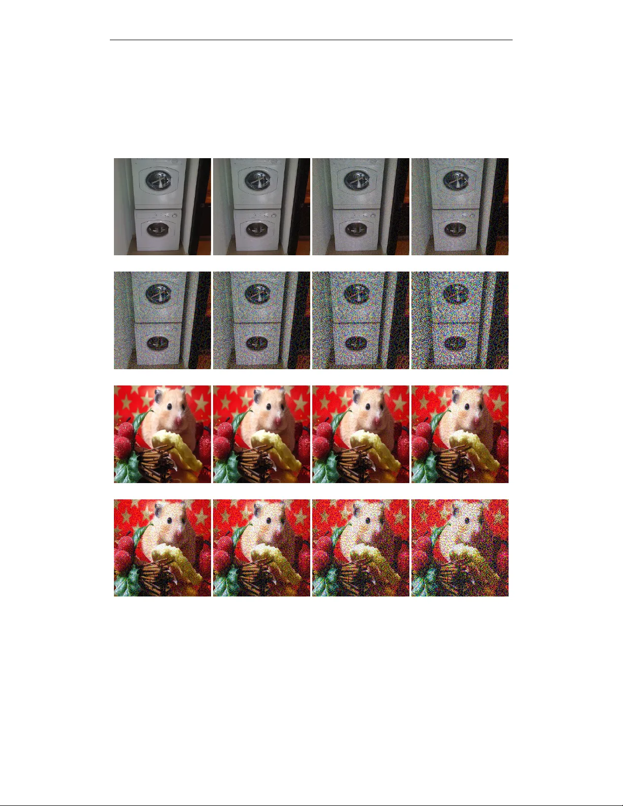
W orkshop track - ICLR 2017 A D V E R S A R I A L E X A M P L E S I N T H E P H Y S I C A L W O R L D Alexey Kurakin Google Brain kurakin@google.com Ian J. Goodfello w OpenAI ian@openai.com Samy Bengio Google Brain bengio@google.com A B S T R AC T Most existing machine learning classifiers are highly vulnerable to adv ersarial examples. An adversarial e xample is a sample of input data which has been mod- ified very slightly in a way that is intended to cause a machine learning classifier to misclassify it. In man y cases, these modifications can be so subtle that a human observer does not even notice the modification at all, yet the classifier still mak es a mistake. Adversarial e xamples pose security concerns because they could be used to perform an attack on machine learning systems, e v en if the adversary has no access to the underlying model. Up to now , all previous work has assumed a threat model in which the adversary can feed data directly into the machine learn- ing classifier . This is not always the case for systems operating in the physical world, for example those which are using signals from cameras and other sensors as input. This paper sho ws that e v en in such physical world scenarios, machine learning systems are vulnerable to adversarial examples. W e demonstrate this by feeding adv ersarial images obtained from a cell-phone camera to an ImageNet In- ception classifier and measuring the classification accuracy of the system. W e find that a large fraction of adv ersarial examples are classified incorrectly e ven when perceiv ed through the camera. 1 I N T RO D U C T I O N (a) Image from dataset (b) Clean image (c) Adv . image,  = 4 (d) Adv . image,  = 8 Figure 1: Demonstration of a black box attack (in which the attack is constructed without access to the model) on a phone app for image classification using physical adversarial examples. W e took a clean image from the dataset (a) and used it to generate adversarial images with various sizes of adversarial perturbation  . Then we printed clean and adversarial images and used the T ensorFlow Camera Demo app to classify them. A clean image (b) is recognized correctly as a “washer” when perceiv ed through the camera, while adversarial images (c) and (d) are misclassified. See video of full demo at https://youtu.be/zQ_uMenoBCk . 1 W orkshop track - ICLR 2017 Recent adv ances in machine learning and deep neural networks enabled researchers to solve multiple important practical problems like image, video, text classification and others (Krizhe vsky et al., 2012; Hinton et al., 2012; Bahdanau et al., 2015). Howe v er , machine learning models are often vulnerable to adversarial manipulation of their input in- tended to cause incorrect classification (Dalvi et al., 2004). In particular , neural networks and man y other cate gories of machine learning models are highly vulnerable to attacks based on small modifi- cations of the input to the model at test time (Biggio et al., 2013; Szegedy et al., 2014; Goodfellow et al., 2014; Papernot et al., 2016b). The problem can be summarized as follows. Let’ s say there is a machine learning system M and input sample C which we call a clean example. Let’ s assume that sample C is correctly classified by the machine learning system, i.e. M ( C ) = y true . It’ s possible to construct an adversarial example A which is perceptually indistinguishable from C but is classified incorrectly , i.e. M ( A ) 6 = y true . These adv ersarial e xamples are misclassified far more often than e xamples that hav e been perturbed by noise, even if the magnitude of the noise is much larger than the magnitude of the adversarial perturbation (Szegedy et al., 2014). Adversarial examples pose potential security threats for practical machine learning applications. In particular, Sze gedy et al. (2014) sho wed that an adversarial example that was designed to be misclassified by a model M 1 is often also misclassified by a model M 2 . This adversarial example transferability property means that it is possible to generate adversarial examples and perform a mis- classification attack on a machine learning system without access to the underlying model. Papernot et al. (2016a) and Papernot et al. (2016b) demonstrated such attacks in realistic scenarios. Howe v er all prior work on adversarial examples for neural networks made use of a threat model in which the attacker can supply input directly to the machine learning model. Prior to this work, it was not known whether adversarial examples would remain misclassified if the examples were constructed in the physical world and observ ed through a camera. Such a threat model can describe some scenarios in which attacks can take place entirely within a computer , such as as ev ading spam filters or malware detectors (Biggio et al., 2013; Nelson et al.). Howe v er , many practical machine learning systems operate in the physical world. Possible exam- ples include but are not limited to: robots perceiving world through cameras and other sensors, video surveillance systems, and mobile applications for image or sound classification. In such scenarios the adversary cannot rely on the ability of fine-grained per-pix el modifications of the input data. The following question thus arises: is it still possible to craft adversarial examples and perform adver - sarial attacks on machine learning systems which are operating in the physical w orld and perceiving data through various sensors, rather than digital representation? Some prior work has addressed the problem of physical attacks against machine learning systems, but not in the context of fooling neural networks by making very small perturbations of the input. For example, Carlini et al. (2016) demonstrate an attack that can create audio inputs that mobile phones recognize as containing intelligible voice commands, but that humans hear as an unintelli- gible voice. Face recognition systems based on photos are vulnerable to replay attacks, in which a previously captured image of an authorized user’ s face is presented to the camera instead of an actual face (Smith et al., 2015). Adversarial examples could in principle be applied in either of these phys- ical domains. An adversarial example for the voice command domain would consist of a recording that seems to be innocuous to a human observer (such as a song) but contains voice commands rec- ognized by a machine learning algorithm. An adversarial example for the face recognition domain might consist of very subtle markings applied to a person’ s face, so that a human observer would recognize their identity correctly , but a machine learning system would recognize them as being a different person. The most similar work to this paper is Sharif et al. (2016), which appeared publicly after our work but had been submitted to a conference earlier . Sharif et al. (2016) also print images of adversarial examples on paper and demonstrated that the printed images fool image recognition systems when photographed. The main differences between their work and ours are that: (1) we use a cheap closed-form attack for most of our experiments, while Sharif et al. (2016) use a more expensi ve attack based on an optimization algorithm, (2) we mak e no particular ef fort to modify our adversarial examples to improve their chances of surviving the printing and photography process. W e simply make the scientific observ ation that v ery many adv ersarial e xamples do survi ve this pro- cess without any intervention. Sharif et al. (2016) introduce extra features to make their attacks work 2 W orkshop track - ICLR 2017 as best as possible for practical attacks against face recognition systems. (3) Sharif et al. (2016) are restricted in the number of pix els the y can modify (only those on the glasses frames) b ut can modify those pix els by a large amount; we are restricted in the amount we can modify a pix el b ut are free to modify all of them. T o in v estigate the extent to which adversarial e xamples survi v e in the physical world, we conducted an e xperiment with a pre-trained ImageNet Inception classifier (Sze gedy et al., 2015). W e generated adversarial examples for this model, then we fed these examples to the classifier through a cell- phone camera and measured the classification accuracy . This scenario is a simple physical world system which perceiv es data through a camera and then runs image classification. W e found that a large fraction of adversarial examples generated for the original model remain misclassified e ven when perceiv ed through a camera. 1 Surprisingly , our attack methodology required no modification to account for the presence of the camera—the simplest possible attack of using adversarial examples crafted for the Inception model resulted in adversarial examples that successfully transferred to the union of the camera and Incep- tion. Our results thus provide a lower bound on the attack success rate that could be achieved with more specialized attacks that explicitly model the camera while crafting the adv ersarial example. One limitation of our results is that we hav e assumed a threat model under which the attacker has full knowledge of the model architecture and parameter values. This is primarily so that we can use a single Inception v3 model in all experiments, without having to devise and train a different high-performing model. The adversarial example transfer property implies that our results could be extended trivially to the scenario where the attacker does not hav e access to the model description (Szegedy et al., 2014; Goodfellow et al., 2014; Papernot et al., 2016b). While we haven’ t run detailed experiments to study transferability of physical adv ersarial examples we were able to build a simple phone application to demonstrate potential adversarial black box attack in the physical world, see fig. 1. T o better understand how the non-trivial image transformations caused by the camera affect adver - sarial example transferability , we conducted a series of additional experiments where we studied how adv ersarial examples transfer across se v eral specific kinds of synthetic image transformations. The rest of the paper is structured as follows: In Section 2, we revie w different methods which we used to generate adversarial examples. This is followed in Section 3 by details about our “physical world” experimental set-up and results. Finally , Section 4 describes our experiments with various artificial image transformations (like changing brightness, contrast, etc...) and how they affect ad- versarial e xamples. 2 M E T H O D S O F G E N E R A T I N G A D V E R S A R I A L I M A G E S This section describes dif ferent methods to generate adversarial examples which we ha ve used in the experiments. It is important to note that none of the described methods guarantees that generated image will be misclassified. Nevertheless we call all of the generated images “adv ersarial images”. In the remaining of the paper we use the following notation: • X - an image, which is typically 3-D tensor (width × height × depth). In this paper, we assume that the values of the pix els are integer numbers in the range [0 , 255] . • y true - true class for the image X . • J ( X , y ) - cross-entropy cost function of the neural network, given image X and class y . W e intentionally omit network weights (and other parameters) θ in the cost func- tion because we assume they are fixed (to the value resulting from training the machine learning model) in the context of the paper . For neural networks with a softmax output layer , the cross-entropy cost function applied to integer class labels equals the negati ve 1 Dileep George noticed that another kind of adversarially constructed input, designed to have no true class yet be categorized as belonging to a specific class, fooled con v olutional networks when photographed, in a less systematic experiments. As of August 19, 2016 it was mentioned in Figure 6 at http://www. evolvingai.org/fooling 3 W orkshop track - ICLR 2017 log-probability of the true class gi ven the image: J ( X , y ) = − log p ( y | X ) , this relation- ship will be used below . • C lip X, { X 0 } - function which performs per-pixel clipping of the image X 0 , so the result will be in L ∞  -neighbourhood of the source image X . The exact clipping equation is as follows: C l ip X, { X 0 } ( x, y, z ) = min n 255 , X ( x, y , z ) + , max  0 , X ( x, y , z ) − , X 0 ( x, y , z )  o where X ( x, y , z ) is the value of channel z of the image X at coordinates ( x, y ) . 2 . 1 F A S T M E T H O D One of the simplest methods to generate adv ersarial images, described in (Goodfello w et al., 2014), is motiv ated by linearizing the cost function and solving for the perturbation that maximizes the cost subject to an L ∞ constraint. This may be accomplished in closed form, for the cost of one call to back-propagation: X adv = X +  sign  ∇ X J ( X , y true )  where  is a hyper -parameter to be chosen. In this paper we refer to this method as “fast” because it does not require an iterative procedure to compute adversarial e xamples, and thus is much faster than other considered methods. 2 . 2 B A S I C I T E R A T I V E M E T H O D W e introduce a straightforward way to extend the “fast” method—we apply it multiple times with small step size, and clip pixel v alues of intermediate results after each step to ensure that the y are in an  -neighbourhood of the original image: X adv 0 = X , X adv N +1 = C lip X, n X adv N + α sign  ∇ X J ( X adv N , y true )  o In our experiments we used α = 1 , i.e. we changed the v alue of each pixel only by 1 on each step. W e selected the number of iterations to be min(  + 4 , 1 . 25  ) . This amount of iterations was chosen heuristically; it is sufficient for the adv ersarial e xample to reach the edge of the  max-norm ball but restricted enough to keep the computational cost of experiments manageable. Below we refer to this method as “basic iterati v e” method. 2 . 3 I T E R AT I V E L E A S T - L I K E L Y C L A S S M E T H O D Both methods we have described so far simply try to increase the cost of the correct class, without specifying which of the incorrect classes the model should select. Such methods are sufficient for application to datasets such as MNIST and CIF AR-10, where the number of classes is small and all classes are highly distinct from each other . On ImageNet, with a much larger number of classes and the varying degrees of significance in the difference between classes, these methods can result in uninteresting misclassifications, such as mistaking one breed of sled dog for another breed of sled dog. In order to create more interesting mistakes, we introduce the iterative least-likely class method . This iterativ e method tries to mak e an adversarial image which will be classified as a specific desired target class. For desired class we chose the least-likely class according to the prediction of the trained network on image X : y LL = arg min y  p ( y | X )  . For a well-trained classifier , the least-likely class is usually highly dissimilar from the true class, so this attack method results in more interesting mistakes, such as mistaking a dog for an airplane. T o make an adversarial image which is classified as y LL we maximize log p ( y LL | X ) by mak- ing iterativ e steps in the direction of sign  ∇ X log p ( y LL | X )  . This last expression equals sign  −∇ X J ( X , y LL )  for neural networks with cross-entropy loss. Thus we have the following procedure: 4 W orkshop track - ICLR 2017 X adv 0 = X , X adv N +1 = C lip X,  X adv N − α sign  ∇ X J ( X adv N , y LL )  For this iterati ve procedure we used the same α and same number of iterations as for the basic iterativ e method. Below we refer to this method as the “least lik ely class” method or shortly “l.l. class”. 2 . 4 C O M P A R I S O N O F M E T H O D S O F G E N E R A T I N G A D V E R S A R I A L E X A M P L E S 0 16 32 48 64 80 96 112 128 epsilon 0.0 0.2 0.4 0.6 0.8 1.0 top-1 accuracy clean images fast adv. basic iter. adv. least likely class adv. 0 16 32 48 64 80 96 112 128 epsilon 0.0 0.2 0.4 0.6 0.8 1.0 top-5 accuracy clean images fast adv. basic iter. adv. least likely class adv. Figure 2: T op-1 and top-5 accuracy of Inception v3 under attack by different adversarial methods and dif ferent  compared to “clean images” — unmodified images from the dataset. The accuracy was computed on all 50 , 000 validation images from the ImageNet dataset. In these experiments  varies from 2 to 128 . As mentioned abov e, it is not guaranteed that an adversarial image will actually be misclassified— sometimes the attacker wins, and sometimes the machine learning model wins. W e did an exper- imental comparison of adversarial methods to understand the actual classification accuracy on the generated images as well as the types of perturbations exploited by each of the methods. The e xperiments were performed on all 50 , 000 validation samples from the ImageNet dataset (Rus- sakovsk y et al., 2014) using a pre-trained Inception v3 classifier (Szegedy et al., 2015). For each validation image, we generated adversarial examples using different methods and different values of  . For each pair of method and  , we computed the classification accuracy on all 50 , 000 images. Also, we computed the accuracy on all clean images, which we used as a baseline. T op-1 and top-5 classification accurac y on clean and adversarial images for v arious adversarial methods are summarized in Figure 2. Examples of generated adversarial images could be found in Appendix in Figures 5 and 4. As shown in Figure 2, the fast method decreases top-1 accuracy by a factor of two and top-5 accuracy by about 40% even with the smallest v alues of  . As we increase  , accuracy on adversarial images generated by the fast method stays on approximately the same level until  = 32 and then slowly decreases to almost 0 as  grows to 128 . This could be explained by the fact that the fast method adds  -scaled noise to each image, thus higher values of  essentially destroys the content of the image and makes it unrecognisable e ven by humans, see Figure 5. On the other hand iterati ve methods e xploit much finer perturbations which do not destro y the image ev en with higher  and at the same time confuse the classifier with higher rate. The basic iterative method is able to produce better adversarial images when  < 48 , howe ver as we increase  it is unable to improve. The “least likely class” method destroys the correct classification of most images ev en when  is relativ ely small. W e limit all further e xperiments to  ≤ 16 because such perturbations are only perceived as a small noise (if perceiv ed at all), and adv ersarial methods are able to produce a significant number of misclassified examples in this  -neighbourhood of clean images. 5 W orkshop track - ICLR 2017 3 P H OT O S O F A D V E R S A R I A L E X A M P L E S 3 . 1 D E S T R U C T I O N R A T E O F A DV E R S A R I A L I M AG E S T o study the influence of arbitrary transformations on adversarial images we introduce the notion of destruction rate. It can be described as the fraction of adversarial images which are no longer misclassified after the transformations. The formal definition is the following: d = P n k =1 C ( X k , y k true ) C ( X k adv , y k true ) C ( T ( X k adv ) , y k true ) P n k =1 C ( X k , y k true ) C ( X k adv , y k true ) (1) where n is the number of images used to comput the destruction rate, X k is an image from the dataset, y k true is the true class of this image, and X k adv is the corresponding adversarial image. The function T ( • ) is an arbitrary image transformation—in this article, we study a variety of transfor- mations, including printing the image and taking a photo of the result. The function C ( X , y ) is an indicator function which returns whether the image was classified correctly: C ( X , y ) =  1 , if image X is classified as y ; 0 , otherwise. W e denote the binary negation of this indicator v alue as C ( X , y ) , which is computed as C ( X , y ) = 1 − C ( X , y ) . 3 . 2 E X P E R I M E N TA L S E T U P (a) Printout (b) Photo of printout (c) Cropped image Figure 3: Experimental setup: (a) generated printout which contains pairs of clean and adversar - ial images, as well as QR codes to help automatic cropping; (b) photo of the printout made by a cellphone camera; (c) automatically cropped image from the photo. T o e xplore the possibility of physical adv ersarial e xamples we ran a series of e xperiments with photos of adversarial e xamples. W e printed clean and adversarial images, took photos of the printed pages, and cropped the printed images from the photos of the full page. W e can think of this as a black box transformation that we refer to as “photo transformation”. W e computed the accuracy on clean and adversarial images before and after the photo transformation as well as the destruction rate of adversarial images subjected to photo transformation. The experimental procedure was as follo ws: 1. Print the image, see Figure 3a. In order to reduce the amount of manual work, we printed multiple pairs of clean and adversarial examples on each sheet of paper . Also, QR codes were put into corners of the printout to facilitate automatic cropping. (a) All generated pictures of printouts (Figure 3a) were sa ved in lossless PNG format. (b) Batches of PNG printouts were conv erted to multi-page PDF file using the con- vert tool from the ImageMagick suite with the default settings: convert * .png output.pdf 6 W orkshop track - ICLR 2017 (c) Generated PDF files were printed using a Ricoh MP C5503 of fice printer . Each page of PDF file was automatically scaled to fit the entire sheet of paper using the default printer scaling. The printer resolution was set to 600dpi. 2. T ake a photo of the printed image using a cell phone camera (Ne xus 5x), see Figure 3b. 3. Automatically crop and warp v alidation examples from the photo, so they would become squares of the same size as source images, see Figure 3c: (a) Detect values and locations of four QR codes in the corners of the photo. The QR codes encode which batch of validation examples is shown on the photo. If detection of an y of the corners failed, the entire photo w as discarded and images from the photo were not used to calculate accuracy . W e observed that no more than 10% of all images were discarded in any experiment and typically the number of discarded images was about 3% to 6% . (b) W arp photo using perspecti ve transform to move location of QR codes into pre-defined coordinates. (c) After the image was warped, each example has known coordinates and can easily be cropped from the image. 4. Run classification on transformed and source images. Compute accuracy and destruction rate of adversarial images. This procedure in v olves manually taking photos of the printed pages, without careful control of lighting, camera angle, distance to the page, etc. This is intentional; it introduces nuisance v ariability that has the potential to destroy adversarial perturbations that depend on subtle, fine co-adaptation of exact pixel values. That being said, we did not intentionally seek out e xtreme camera angles or lighting conditions. All photos were taken in normal indoor lighting with the camera pointed approximately straight at the page. For each combination of adversarial example generation method and  we conducted two sets of experiments: • A verage case. T o measure the av erage case performance, we randomly selected 102 images to use in one experiment with a gi v en  and adversarial method. This experiment estimates how often an adversary would succeed on randomly chosen photos—the world chooses an image randomly , and the adversary attempts to cause it to be misclassified. • Prefilter ed case. T o study a more aggressiv e attack, we performed experiments in which the images are prefiltered. Specifically , we selected 102 images such that all clean images are classified correctly , and all adversarial images (before photo transformation) are clas- sified incorrectly (both top-1 and top-5 classification). In addition we used a confidence threshold for the top prediction: p ( y predicted | X ) ≥ 0 . 8 , where y predicted is the class pre- dicted by the network for image X . This experiment measures how often an adversary would succeed when the adversary can choose the original image to attack. Under our threat model, the adversary has access to the model parameters and architecture, so the attacker can always run inference to determine whether an attack will succeed in the ab- sence of photo transformation. The attacker might expect to do the best by choosing to make attacks that succeed in this initial condition. The victim then tak es a ne w photo of the physical object that the attacker chooses to display , and the photo transformation can either preserve the attack or destroy it. 3 . 3 E X P E R I M E N TA L R E S U LT S O N P H O T O S O F A DV E R S A R I A L I M A G E S Results of the photo transformation experiment are summarized in T ables 1, 2 and 3. W e found that “fast” adversarial images are more robust to photo transformation compared to itera- tiv e methods. This could be explained by the fact that iterative methods exploit more subtle kind of perturbations, and these subtle perturbations are more likely to be destroyed by photo transforma- tion. One unexpected result is that in some cases the adversarial destruction rate in the “prefiltered case” was higher compared to the “average case”. In the case of the iterative methods, ev en the total 7 W orkshop track - ICLR 2017 T able 1: Accuracy on photos of adversarial images in the a verage case (randomly chosen images). Photos Source images Adversarial Clean images Adv . images Clean images Adv . images method top-1 top-5 top-1 top-5 top-1 top-5 top-1 top-5 fast  = 16 79.8% 91.9% 36.4% 67.7% 85.3% 94.1% 36.3% 58.8% fast  = 8 70.6% 93.1% 49.0% 73.5% 77.5% 97.1% 30.4% 57.8% fast  = 4 72.5% 90.2% 52.9% 79.4% 77.5% 94.1% 33.3% 51.0% fast  = 2 65.7% 85.9% 54.5% 78.8% 71.6% 93.1% 35.3% 53.9% iter . basic  = 16 72.9% 89.6% 49.0% 75.0% 81.4% 95.1% 28.4% 31.4% iter . basic  = 8 72.5% 93.1% 51.0% 87.3% 73.5% 93.1% 26.5% 31.4% iter . basic  = 4 63.7% 87.3% 48.0% 80.4% 74.5% 92.2% 12.7% 24.5% iter . basic  = 2 70.7% 87.9% 62.6% 86.9% 74.5% 96.1% 28.4% 41.2% l.l. class  = 16 71.1% 90.0% 60.0% 83.3% 79.4% 96.1% 1.0% 1.0% l.l. class  = 8 76.5% 94.1% 69.6% 92.2% 78.4% 98.0% 0.0% 6.9% l.l. class  = 4 76.8% 86.9% 75.8% 85.9% 80.4% 90.2% 9.8% 24.5% l.l. class  = 2 71.6% 87.3% 68.6% 89.2% 75.5% 92.2% 20.6% 44.1% T able 2: Accuracy on photos of adversarial images in the prefiltered case (clean image correctly classified, adversarial image confidently incorrectly classified in digital form being being printed and photographed ). Photos Source images Adversarial Clean images Adv . images Clean images Adv . images method top-1 top-5 top-1 top-5 top-1 top-5 top-1 top-5 fast  = 16 81.8% 97.0% 5.1% 39.4% 100.0% 100.0% 0.0% 0.0% fast  = 8 77.1% 95.8% 14.6% 70.8% 100.0% 100.0% 0.0% 0.0% fast  = 4 81.4% 100.0% 32.4% 91.2% 100.0% 100.0% 0.0% 0.0% fast  = 2 88.9% 99.0% 49.5% 91.9% 100.0% 100.0% 0.0% 0.0% iter . basic  = 16 93.3% 97.8% 60.0% 87.8% 100.0% 100.0% 0.0% 0.0% iter . basic  = 8 89.2% 98.0% 64.7% 91.2% 100.0% 100.0% 0.0% 0.0% iter . basic  = 4 92.2% 97.1% 77.5% 94.1% 100.0% 100.0% 0.0% 0.0% iter . basic  = 2 93.9% 97.0% 80.8% 97.0% 100.0% 100.0% 0.0% 1.0% l.l. class  = 16 95.8% 100.0% 87.5% 97.9% 100.0% 100.0% 0.0% 0.0% l.l. class  = 8 96.0% 100.0% 88.9% 97.0% 100.0% 100.0% 0.0% 0.0% l.l. class  = 4 93.9% 100.0% 91.9% 98.0% 100.0% 100.0% 0.0% 0.0% l.l. class  = 2 92.2% 99.0% 93.1% 98.0% 100.0% 100.0% 0.0% 0.0% T able 3: Adversarial image destruction rate with photos. Adversarial A verage case Prefiltered case method top-1 top-5 top-1 top-5 fast  = 16 12.5% 40.0% 5.1% 39.4% fast  = 8 33.3% 40.0% 14.6% 70.8% fast  = 4 46.7% 65.9% 32.4% 91.2% fast  = 2 61.1% 63.2% 49.5% 91.9% iter . basic  = 16 40.4% 69.4% 60.0% 87.8% iter . basic  = 8 52.1% 90.5% 64.7% 91.2% iter . basic  = 4 52.4% 82.6% 77.5% 94.1% iter . basic  = 2 71.7% 81.5% 80.8% 96.9% l.l. class  = 16 72.2% 85.1% 87.5% 97.9% l.l. class  = 8 86.3% 94.6% 88.9% 97.0% l.l. class  = 4 90.3% 93.9% 91.9% 98.0% l.l. class  = 2 82.1% 93.9% 93.1% 98.0% 8 W orkshop track - ICLR 2017 success rate was lower for prefiltered images rather than randomly selected images. This suggests that, to obtain very high confidence, iterativ e methods often make subtle co-adaptations that are not able to surviv e photo transformation. Overall, the results show that some fraction of adversarial examples stays misclassified even after a non-trivial transformation: the photo transformation. This demonstrates the possibility of physical adversarial examples. For example, an adversary using the fast method with  = 16 could expect that about 2 / 3 of the images would be top-1 misclassified and about 1 / 3 of the images would be top-5 misclassified. Thus by generating enough adversarial images, the adversary could expect to cause far more misclassification than would occur on natural inputs. 3 . 4 D E M O N S T R A T I O N O F B L AC K B OX A D V E R S A R I A L A T TAC K I N T H E P H Y S I C A L W O R L D The experiments described above study physical adversarial examples under the assumption that adversary has full access to the model (i.e. the adv ersary kno ws the architecture, model weights, etc . . . ). Howe ver , the black box scenario, in which the attacker does not hav e access to the model, is a more realistic model of many security threats. Because adversarial examples often transfer from one model to another, they may be used for black box attacks Szegedy et al. (2014); Papernot et al. (2016a). As our own black box attack, we demonstrated that our physical adversarial examples fool a different model than the one that was used to construct them. Specifically , we showed that they fool the open source T ensorFlo w camera demo 2 — an app for mobile phones which performs image classification on-device. W e showed several printed clean and adversarial images to this app and observed change of classification from true label to incorrect label. V ideo with the demo av ailable at https://youtu.be/zQ_uMenoBCk . W e also demonstrated this ef fect li ve at GeekPwn 2016. 4 A RT I FI C I A L I M A G E T R A N S F O R M A T I O N S The transformations applied to images by the process of printing them, photographing them, and cropping them could be considered as some combination of much simpler image transformations. Thus to better understand what is going on we conducted a series of experiments to measure the adversarial destruction rate on artificial image transformations. W e explored the following set of transformations: change of contrast and brightness, Gaussian blur , Gaussian noise, and JPEG en- coding. For this set of experiments we used a subset of 1 , 000 images randomly selected from the validation set. This subset of 1 , 000 images was selected once, thus all experiments from this section used the same subset of images. W e performed experiments for multiple pairs of adversarial method and transformation. For each given pair of transformation and adv ersarial method we computed adversarial examples, applied the transformation to the adversarial examples, and then computed the destruction rate according to Equation (1). Detailed results for various transformations and adversarial methods with  = 16 could be found in Appendix in Figure 6. The following general observ ations can be drawn from these e xperiments: • Adversarial e xamples generated by the fast method are the most robust to transformations, and adversarial examples generated by the iterative least-likely class method are the least robust. This coincides with our results on photo transformation. • The top-5 destruction rate is typically higher than top-1 destruction rate. This can be ex- plained by the fact that in order to “destroy” top-5 adversarial examples, a transformation has to push the correct class labels into one of the top-5 predictions. Howe v er in order to destroy top-1 adv ersarial e xamples we hav e to push the correct label to be top-1 prediction, which is a strictly stronger requirement. • Changing brightness and contrast does not af fect adv ersarial examples much. The destruc- tion rate on fast and basic iterative adversarial examples is less than 5% , and for the iterati ve least-likely class method it is less than 20% . 2 As of October 25, 2016 T ensorFlow camera demo was a vailable at https://github.com/ tensorflow/tensorflow/tree/master/tensorflow/examples/android 9 W orkshop track - ICLR 2017 • Blur , noise and JPEG encoding have a higher destruction rate than changes of brightness and contrast. In particular, the destruction rate for iterative methods could reach 80% − 90% . Howe v er none of these transformations destroy 100% of adversarial examples, which coincides with the “photo transformation” experiment. 5 C O N C L U S I O N In this paper we explored the possibility of creating adversarial examples for machine learning sys- tems which operate in the physical world. W e used images taken from a cell-phone camera as an input to an Inception v3 image classification neural network. W e sho wed that in such a set-up, a sig- nificant fraction of adversarial images crafted using the original network are misclassified e v en when fed to the classifier through the camera. This finding demonstrates the possibility of adversarial ex- amples for machine learning systems in the physical world. In future work, we expect that it will be possible to demonstrate attacks using other kinds of physical objects besides images printed on paper , attacks against different kinds of machine learning systems, such as sophisticated reinforce- ment learning agents, attacks performed without access to the model’ s parameters and architecture (presumably using the transfer property), and physical attacks that achiev e a higher success rate by explicitly modeling the phyiscal transformation during the adversarial example construction process. W e also hope that future work will de velop ef fecti ve methods for defending ag ainst such attacks. R E F E R E N C E S Dzmitry Bahdanau, K yunghyun Cho, and Y oshua Bengio. Neural machine translation by jointly learning to align and translate. In ICLR’2015, , 2015. Battista Biggio, Igino Corona, Davide Maiorca, Blaine Nelson, Nedim ˇ Srndi ´ c, Pavel Lasko v , Gior - gio Giacinto, and Fabio Roli. Evasion attacks against machine learning at test time. In J oint Eur opean Conference on Machine Learning and Knowledge Discovery in Databases , pp. 387– 402. Springer , 2013. Nicholas Carlini, Pratyush Mishra, T avish V aidya, Y uankai Zhang, Micah Sherr, Clay Shields, Da vid W agner , and W enchao Zhou. Hidden voice commands. In 25th USENIX Security Symposium (USENIX Security 16) , Austin, TX, August 2016. USENIX Association. URL https://www.usenix.org/conference/usenixsecurity16/ technical- sessions/presentation/carlini . Nilesh Dalvi, Pedro Domingos, Sumit Sanghai, Deepak V erma, et al. Adversarial classification. In Pr oceedings of the tenth A CM SIGKDD international confer ence on Knowledge discovery and data mining , pp. 99–108. A CM, 2004. Ian J. Goodfello w , Jonathon Shlens, and Christian Szegedy . Explaining and harnessing adversarial examples. CoRR , abs/1412.6572, 2014. URL . Geoffre y Hinton, Li Deng, Dong Y u, George Dahl, Abdel rahman Mohamed, Navdeep Jaitly , An- drew Senior , V incent V anhoucke, Patrick Nguyen, T ara Sainath, and Brian Kingsbury . Deep neural networks for acoustic modeling in speech recognition. Signal Pr ocessing Magazine , 2012. Alex Krizhe vsky , Ilya Sutskev er , and Geoffrey Hinton. ImageNet classification with deep conv olu- tional neural networks. In Advances in Neural Information Pr ocessing Systems 25 (NIPS’2012) . 2012. Blaine Nelson, Marco Barreno, Fuching Jack Chi, Anthony D Joseph, Benjamin IP Rubinstein, Udam Saini, Charles A Sutton, J Doug T ygar , and Kai Xia. Exploiting machine learning to subv ert your spam filter . N. P apernot, P . McDaniel, and I. Goodfellow . T ransferability in Machine Learning: from Phe- nomena to Black-Box Attacks using Adversarial Samples. ArXiv e-prints , May 2016b . URL http://arxiv.org/abs/1605.07277 . 10 W orkshop track - ICLR 2017 Nicolas Papernot, Patrick Drew McDaniel, Ian J. Goodfellow , Somesh Jha, Z. Berkay Celik, and Ananthram Swami. Practical black-box attacks against deep learning systems using adversarial examples. CoRR , abs/1602.02697, 2016a. URL . Olga Russako vsky , Jia Deng, Hao Su, Jonathan Krause, Sanjee v Satheesh, Sean Ma, Zhiheng Huang, Andrej Karpathy , Aditya Khosla, Michael Bernstein, et al. Imagenet large scale visual recognition challenge. arXiv pr eprint arXiv:1409.0575 , 2014. Mahmood Sharif, Sruti Bhagav atula, Lujo Bauer, and Michael K. Reiter . Accessorize to a crime: Real and stealthy attacks on state-of-the-art face recognition. In Pr oceedings of the 23rd ACM SIGSA C Conference on Computer and Communications Security , October 2016. T o appear . Daniel F Smith, Arnold W iliem, and Brian C Lovell. Face recognition on consumer devices: Re- flections on replay attacks. IEEE T ransactions on Information F or ensics and Security , 10(4): 736–745, 2015. Christian Szegedy , W ojciech Zaremba, Ilya Sutskev er , Joan Bruna, Dumitru Erhan, Ian J. Goodfel- low , and Rob Fergus. Intriguing properties of neural networks. ICLR , abs/1312.6199, 2014. URL http://arxiv.org/abs/1312.6199 . Christian Szegedy , V incent V anhoucke, Serge y Ioffe, Jonathon Shlens, and Zbigniew W ojna. Re- thinking the inception architecture for computer vision. CoRR , abs/1512.00567, 2015. URL http://arxiv.org/abs/1512.00567 . 11 W orkshop track - ICLR 2017 A ppendix Appendix contains following figures: 1. Figure 4 with examples of adv ersarial images produced by dif ferent adversarial methods. 2. Figure 5 with examples of adv ersarial images for v arious v alues of  . 3. Figure 6 contain plots of adversarial destruction rates for v arious image transformations. Clean image “Fast”; L ∞ distance to clean image = 32 “Basic iter . ”; L ∞ distance to clean image = 32 “L.l. class”; L ∞ distance to clean image = 28 Figure 4: Comparison of different adversarial methods with  = 32 . Perturbations generated by iterativ e methods are finer compared to the f ast method. Also iterati v e methods do not alw ays select a point on the border of  -neighbourhood as an adversarial image. 12 W orkshop track - ICLR 2017 clean image  = 4  = 8  = 16  = 24  = 32  = 48  = 64 clean image  = 4  = 8  = 16  = 24  = 32  = 48  = 64 Figure 5: Comparison of images resulting from an adversarial pertubation using the “fast” method with different size of perturbation  . The top image is a “washer” while the bottom one is a “ham- ster”. In both cases clean images are classified correctly and adversarial images are misclassified for all considered  . 13 W orkshop track - ICLR 2017 30 20 10 0 10 20 30 b r i g h t n e s s + X 0.0% 2.0% 4.0% 6.0% 8.0% 10.0% 12.0% 14.0% 16.0% 18.0% destruction rate (a) Change of brightness 0.7 0.8 0.9 1.0 1.1 1.2 c o n t r a s t ∗ X 0.0% 5.0% 10.0% 15.0% 20.0% destruction rate (b) Change of contrast 0.4 0.6 0.8 1.0 1.2 1.4 1.6 1.8 2.0 G a u s s i a n b l u r σ 0.0% 20.0% 40.0% 60.0% 80.0% 100.0% destruction rate (c) Gaussian blur 5 10 15 20 G a u s s i a n n o i s e σ 0.0% 20.0% 40.0% 60.0% 80.0% 100.0% destruction rate (d) Gaussian noise 10 20 30 40 50 60 70 80 90 100 Jpeg quality 0.0% 20.0% 40.0% 60.0% 80.0% 100.0% destruction rate (e) JPEG encoding fast adv., top-1 fast adv., top-5 basic iter. adv., top-1 basic iter. adv., top-5 least likely class adv., top-1 least likely class adv., top-5 Figure 6: Comparison of adversarial destruction rates for various adversarial methods and types of transformations. All experiments were done with  = 16 . 14