BFDA: A Matlab Toolbox for Bayesian Functional Data Analysis

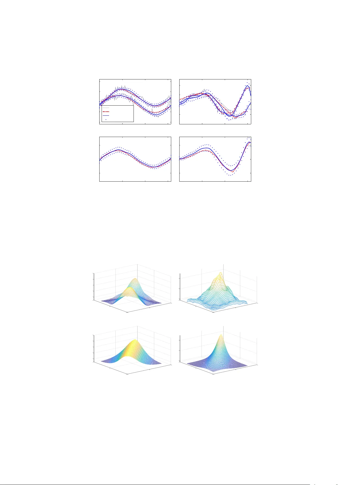
J S S Journal of Statistical Software MMMMMM YYYY, V olume VV, Issue II. doi: 10.18637/jss.v000.i00 BFD A : A MA TLAB T o olb o x for Ba y esian F unctional Data Analysis Jing jing Y ang Univ ersit y of Mic higan P eng Ren Sun trust Banks, Inc. Abstract W e pro vide a MA TLAB to olbox, BFD A , that implements a Bay esian hierarc hical mo del to smo oth multiple functional data with the assumptions of the same underlying Gaussian process distribution, a Gaussian process prior for the mean function, and an In verse-Wishar t pro cess prior for the cov ariance function. This mo del-based approac h can borrow strength from all functional data to increase the smo othing accuracy , as well as estimate the mean-cov ariance func tions sim ultaneously . An option of approximating the Bay esian inference pro cess using cubic B-spline basis functions is integrated in BFD A , which allows for efficiently dealing with high-dimensional functional data. Examples of using BFDA in v arious scenarios and conducting follow-up functional regression are provided. The adv antages of BFDA include: (1) Simul taneously smo oths m ultiple functional data and estimates t he mean-cov ariance functions in a nonparametric wa y; (2) flexibly deals with sparse and high-dimensional functional data with stationary and nonstationary cov ariance functions, and without the requirement of common observ ation grids; (3) provides accurately smo othed functional data for follo w-up analysis. Keywor ds : functional data analysis, Ba yes ian hierarch ical mo del, Gaussian process, In v erse-Wishart pro cess, MA TLAB . 1. Int ro duction Since Ramsay and Dalzell ( 1991 ) first coined the term “functional data analysis” (FD A) for analyzing data that are realizations of a contin uous function, man y statistical metho ds and to ols hav e been proposed for FDA. F or examples, Gra v es et al. ( 2010 ) provided b oth R pac k age fda ( Ramsay et al. 2014 ) and MA TLAB pac k age fdaM ( Ramsay 2014 ) for standard functional data analysis ( Ramsa y and Silv erman 2002 , 2005 ); F ebrero-Bande and de la F uente ( 2012 ) pro vided R pack age fda.usc for implementing nonparametric functional data 2 BFD A : Bay esian F unctional Data Analysis analysis metho ds ( Vieu and F errat y 2006 ) with fda ( Ramsay et al. 2014 ); Y ao et al. ( 2005a , b ) dev elop ed the k ey technique of F unctional Principal Comp onen t Analysis (FPCA) for analyzing sparse functional data, accompanied b y the MA TLAB pac k age P A CE ( Y ao et al. 2015 ); Crainicean u and Goldsmith ( 2010 ) prop osed insights ab out implementing the standard Bay esian FDA using WinBUGS ( Sturtz et al. 2005 ); and Shi and Cheng ( 2014 ) deriv ed R pack age GPFDA for applying the Bay esian nonparametric Gaussian pro cess (GP) regression mo dels ( Shi and Choi 2011 ). Ho wev er, the smo othing step that constructs functions from noisy discrete data has b een neglected b y most of the existing FD A metho ds and to ols, where functional represen tations are integrated in the analyzing mo dels. On the other hand, most of the existing smo othing metho ds pro cess functional samples individually (e.g., cubic smo othin g spline (CSS) and kernel smo othing ( Green and Silve rman 1993 ; Ramsa y and Silv erman 2005 )), whic h is lik ely to induce bias when functional samples are of the same distribution. Here, we pro vide a MA TLAB to olbox BFD A for simult aneously smo othing m ultiple functional observ ations from the same distribution and estimating the underlying mean-co v ariance functions, using a nonparametric Bay esian Hierarc hical Mo del (BHM) with Gaussian-Wishart pro cesses ( Y ang et al. 2016 ). This mo del-based approach b orro ws strength through mo deling the shared mean-cov ariance functions, thus pro ducing more accurate smo othing results than the individually smo othing metho ds ( Y ang et al. 2016 ). Moreo v er, BFD A is flexible for analyzing sparse and dense functional data without the requiremen t of common observ ation grids, suitable for analyzing functional data with b oth stationary and nonstationary cov ariance functions, and efficient for high-dimensional functional data using a Bay esian framework with Approximations by Basis F unctions (BABF) ( Y ang et al. 2015 ). In addition, BFDA provides options for implemen ting the standard Bay esian GP regression metho d, conducting Bay esian principal comp onen t analysis, and using the fdaM pack age for follow-up FD A. In the following context, we first review the BHM and BABF metho ds in Section 2 , and then pro vide examples using BFD A with sim ulated data in Section 3 . In Section 4 , we compare the functional linear regression results by fdaM using the smo othed data b y BFDA and CSS. Last, we conclude w ith a discussion in Section 5 . Details of input options and outputs, as w ell as example MA TLAB scripts of generating the simulation results in this pap er, are provided in the App endix. 2. Metho ds o v erview 2.1. BHM Consider functional data { X i ( t ); t ∈ T , i = 1 , 2 , · · · , n } that are generated from the same sto c hastic pro cess with indep enden t measuremen t errors. In order to simultaneously smooth all noisy observ ations and estimate mean-co v ariance functions, Y ang et al. ( 2016 ) prop osed the following Bay esian Hierarc hical Mo del (BHM) with Gaussian-Wishart pro cesses : X i ( t ) = Z i ( t ) +  i ( t ); Z i ( · ) ∼ GP ( µ Z ( · ) , Σ Z ( · , · )) ,  i ( · ) ∼ N (0 , σ 2  ); (1) µ Z ( · ) | Σ Z ( · , · ) ∼ GP  µ 0 ( · ) , 1 c Σ Z ( · , · )  , Σ Z ( · , · ) ∼ I W P ( δ, σ 2 s A ( · , · )) , σ 2  ∼ I G ( a  , b  ); Journal of Statistical Softw are 3 σ 2 s ∼ I G ( a s , b s ); where { Z i ( t ); i = 1 , · · · , n } denotes the underlying true functional data following the same GP distribution with mean function µ Z ( · ) and co v ariance function Σ Z ( · , · ), I W P denotes the In v erse-Wishart process (IWP) prior ( Da wid 1981 ) for the cov ariance function, I G denotes the Inv erse-Gamma prior, and ( µ 0 ( · ) , c, δ, A ( · , · ) , a  , b  , a s , b s ) are hyper-parameters to b e determined. The IWP prior on Σ Z ( · , · ) mo dels the cov ariance function nonparametrically and therefore makes the BHM metho d suitable for analyzing functional data with unkno wn stationary and nonstationary co v ariance structures. The hyper parameter σ 2 s pro vides the flexibility of estimating the scale of the cov ariance structure in the IWP prior from the data. F or the h yp er-parameter setup, we take µ 0 ( · ) as the smo othed empirical mean estimate, c as 1 for the same data v ariation on the mean function, δ as 5 for noninformative prior on the v ariance function, and determine ( a  , b  , a s , b s ) b y matc hing the h yp er-prior moment s with the empirical estimates. In addition, A ( · , · ) can b e taken as the Mat´ ern correlation ke rnel for analyzing functional data with stationary cov ariance (default in BFDA ), Matern cor ( d ; ρ, ν ) = 1 Γ( ν )2 ν − 1  √ 2 ν d ρ  ν K ν  √ 2 ν d ρ  , d ≥ 0 , ρ > 0 , ν > 0 , where d denotes the distance b et ween tw o grid p oin ts, ρ is the scale parameter, ν is the order of smo othness, and K ν ( · ) is the mo dified Bessel function of the second kind; while as an smo othed empirical co v ariance estimate for analyzing functional data with nonstationary co v ariance. Although the BHM is constructed with infinite-dimensional Gaussian-Wishart pro cesses, practical p osterior inference will b e conducted in a finite manner, e.g., on the observ ation grids { t i } , p ooled grid t = ∪ n i =1 t i , or other ev aluation grids. F or accommo dating uncommon observ ation grids, esp ecially sparsely observ ed data, BHM ev aluates data functions and mean-co v ariance functions on the p ooled grid, while estimating the unobserved functional data by conditioning on the observ ations (similarly as P A CE ). Denoting X i ( t i ) by X t i , Z i ( t i ) by Z t i , µ 0 ( t ) by µ 0 , µ Z ( t ) by µ Z , Σ Z ( t , t ) b y Σ Z , and A ( t , t ) b y A , BHM conducts Bay esian inference for ( { Z i ( t ) } , µ Z , Σ Z , σ 2  , σ 2 s ) by the Mon te Carlo Mark o v Chain (MCMC) algorithm (essentially a Gibbs sampler ( Geman and Geman 1984 )) as follows (refer to Y ang et al. ( 2016 ) for details): Step 0: Set initial v alues. Set hyper-parameters ( c, µ 0 , ν, ρ, a  , b  , a s , b s ). T ake ( µ , σ 2  ) as the empirical estimates, { Z t i } as the raw data { X t i } , and Σ Z as an iden tit y matrix. Step 1: Conditioning on { X t i } and ( µ Z , Σ Z ), up date { Z i ( t ) } from the corresp ondin g conditional mu ltiv ariate normal (MN) distributions; Step 2: Conditioning on { X t i } and { Z t i } , update the noise v ariance σ 2  from the conditional Inv erse-Gamma (IG) distribution; Step 3: Conditional on { Z i ( t ) } and Σ Z , up date µ Z from the conditional MN distribution; Step 4: Conditioning on { Z i ( t ) } and µ Z , up date Σ Z from the conditional In v erse-Wishart (IW) distribution; 4 BFD A : Bay esian F unctional Data Analysis Step 5: Conditioning on Σ Z , Up date σ 2 s from the conditional Gamma distribution. Sp ecifically , the av erages of p osterior samples of { Z i ( t ) , µ Z , Σ Z } are taken as estimates for functional signals and mean-cov ariance functions. In addition, BFDA uses existing MA TLAB pack age mcmcdiag ( S ¨ arkk ¨ a and Aki 2014 ) to diagnosis the MCMC conv ergence b y p oten tial scale reduction factor (PSRF) ( Gelman and Rubin 1992 ), and implemen ts the metho d prop osed by Y uan and Johnson ( 2012 ) with the piv otal discrepancy measures (PDM) of standardized residuals for the go odness-of-fit diagnosis of the assumed mo del. 2.2. BABF Because BHM ( Y ang et al. 2016 ) has computational complexity O ( np 3 m ) with n samples, p p ooled-grid p oin ts, and m MCMC iterations, the metho d encounters computational b ottlenec k for analyzing functional data with large p o oled-grid dimension p . T o resolv e this computational b ottlenec k issue with high-dimensional data, BFD A enables the option of using the BABF metho d prop osed by Y ang et al. ( 2015 ), in which the p osterior inference in BHM is conducted with appro ximations using basis functions. Here, we briefly outline the BABF metho d. First select a w orking grid based on data density , τ = ( τ 1 , τ 2 , · · · , τ L ) > ⊂ T , L << p , then appro ximate { Z i ( τ ) } by a system of basis functions (e.g., cubic B-splines). Let B ( · ) = [ b 1 ( · ) , b 2 ( · ) , · · · , b K ( · )] denote K selected basis functions with co efficien ts ζ i = ( ζ i 1 , ζ i 2 , · · · , ζ iK ) > , then Z i ( τ ) = P K k =1 ζ ik b k ( τ ) = B ( τ ) ζ i . Generally , K can b e selected as L , then ζ i = B ( τ ) − 1 Z i ( τ ), a linear transformation of Z i ( τ ). Note that ev en if B ( τ ) is singular or non-square, ζ i can still b e written as a linear transformation of Z i ( τ ), e.g., using the generalized in verse ( James 1978 ) of B ( τ ) . Because ζ i is a linear transformation of Z i ( τ ) that follo ws a MN distribution under the assumptions in Equation 1 , the induced Bay esian hierarc hical mo del for { ζ i } is derived as ζ i ∼ M N ( µ ζ , Σ ζ ); µ ζ = B ( τ ) − 1 µ Z ( τ ); Σ ζ = B ( τ ) − 1 Σ Z ( τ , τ ) B ( τ ) −> . (2) F urther, from the assumed priors of ( µ Z ( · ) , Σ Z ( · , · )) in Equation 1 , with Ψ( τ , τ ) = σ 2 s A ( τ , τ ), the following priors of ( µ ζ , Σ ζ ) are also induced: µ ζ | Σ ζ ∼ M N  B ( τ ) − 1 µ 0 ( τ ) , c Σ ζ  ; (3) Σ ζ ∼ I W ( δ, B ( τ ) − 1 Ψ( τ , τ ) B ( τ ) −> ) . Then, the BABF approach has computation complexit y O ( nK 3 m ) with the following MCMC algorithm (refer to Y ang et al. ( 2015 ) for details): Step 0: Set initial v alues similarly as in BHM. Set hyper-parameters ( c, µ 0 , ν, ρ, a  , b  , a s , b s ). T ak e ( µ Z ( τ ) , Σ Z ( τ , τ ) , σ 2  ) as empirical estimates, inducing the initial v alues for ( µ ζ , Σ ζ ) by Equation 2 . Step 1: Conditioning on { X t i } and ( µ ζ , Σ ζ , σ 2  ), up date { ζ i } from the conditional MN distribution. Step 2: Conditioning on { ζ i } , up date µ ζ and Σ ζ resp ectiv ely from the conditional MN and IW distributions. Journal of Statistical Softw are 5 Step 3: Conditioning on ( { ζ i } , µ ζ , Σ ζ ), approximate { Z t i , µ Z ( t i ), Σ Z ( t i , t i ), Σ Z ( τ , t i ) , Σ Z ( t i , τ ) , Σ Z ( τ , τ ) } by Z t i = B ( t i ) ζ i , µ Z ( t i ) = B ( t i ) µ ζ , Σ Z ( t i , t i ) = B ( t i )Σ ζ B ( t i ) > , Σ Z ( τ , t i ) > = Σ Z ( t i , τ ) = B ( t i )Σ ζ B ( τ ) > , Σ Z ( τ , τ ) = B ( τ )Σ ζ B ( τ ) > . Step 4: Conditioning on { Z t i } and { X t i } , up date σ 2  b y the conditional IG distribution; Step 5: Conditioning on Σ Z ( τ , τ ), up date σ 2 s b y the conditional Gamma distribution. As a result, the posterior estimates of ( { ζ i } , µ ζ , Σ ζ ) are given by the av erages of the MCMC samples, which are then used to estimate { Z t i , µ Z ( t i ), Σ Z ( t i , t i ) } b y the appro ximation form ulas in Step 3. 2.3. Basis-functio n construction BFD A uses the existing MA TLAB pack age bspline ( Hun yadi 2010 ) to construct B-spline basis functions, using the optimal knot sequence for in terp olation at the working grid τ . The optimal knot sequence is generated by the MA TLAB function optknt ( Gaffney and Po w ell 1976 ; Micc helli et al. 1976 ; de Bo or 1977 ). Y ang et al. ( 2015 ) instructed selecting τ to represen t data densities ( L maybe selected by grid search with test data), such as taking the  100 L +1 , · · · , L × 100 L +1  p ercen tiles of the p o oled grid, or the equally-spaced grid for ev enly distributed data. 3. Examples with sim ulated data In this Section, w e provide examples of using BFDA to analyze simulated functional data with stationary and nonstationary cov ariance functions, common and uncommon (sparse) observ ation grids, as w ell as random observ ation grids. The simulation data used for the example results were generated with n =30, p =40, au =0, bu = π / 2, s = √ 5, r =2, nu =3.5, rho =0.5, dense =0.6, and pgrid as the equally spaced grid ov er (0 , π / 2) with length 40. 3.1. Sim ulate functional data BFD A provides the conv enience of generating sim ulated functional data from the same GP with mean function µ ( t ) = 3 sin (4 t ), stationary co v ariance function s 2 Matern cor ( d ; ρ, ν ), and noises ∼ N (0 , ( s/r ) 2 ) by > GausFD_cgrid = sim_gfd(pgrid, n, s, r, nu, rho, dense, cgrid, stat); where pgrid denotes the p ooled grid, n denotes the num ber of functional samples, r denotes the signal to noise ratio (i.e., the ratio b et wee n the signal and noise standard deviations), rho denotes the Mat´ ern scale parameter, nu denotes the Mat ´ ern order of smo othness. Here, cgrid is a b oolean indicator that controls the output as either common-grid data on pgrid ( cgrid =1) or uncommon-grid data with a randomly selected prop ortion (given by dense ) of the full data on pgrid ( cgrid =0). In addition, stat =1 sp ecifies simulati ng stationary data from GP (3 sin (4 t ) , s 2 Matern cor ( d ; ρ, ν )), while stat =0, sp ecifies simulating data from a nonlinearly transformed GP wi th mean function µ ( t ) = 3( t + 0 . 5) sin (4 t 2 / 3 ) and nons tationary co v ariance function Σ( t, t 0 ) = s 2 ( t + 0 . 5)( t 0 + 0 . 5)Matern cor ( | t 2 / 3 − t 0 2 / 3 | ; ρ, ν ) . 6 BFD A : Bay esian F unctional Data Analysis Let p denote th e l ength of pgrid . The output GausFD_cgrid is a data structure consisted with a cell of true data (Xtrue cell 1 × n ), a cell of noisy data (Xraw cell 1 × n ), a cell of observ ation grids (Tcell 1 × n ), a true co v ariance matrix on pgrid (Cov true p × p ), and a true mean vector on pgrid (Mean true 1 × p ). 3.2. Analyze stationary data by BHM Common grids First, we need to setup the required parameter structure by function setOptions_bfda . F or example, to analy ze functional data wi th common observ ation grids and stationary co v ariance function by BHM, the structure param can b e set as > param = setOptions_bfda(’smeth od’, ’bhm’, ’cgrid’, 1, ’mat’, 1, ’M’, 10000, ’Burnin’, 2000, ’w’, 1, ’ws’, 1); where each parameter is follo wed b y its v alue, and unsp ecified parameters are tak en as default v alues (App endix A.1.). Sp ecifically , smethod=’bhm’ denotes using the BHM metho d; cgrid=1 denotes the analyzed data are of common-grid; mat=1 denotes taking A ( · , · ) in Equation 1 as the Mat´ ern correlation function; M=10000 denotes the num ber of MCMC iterations; Burnin=2000 denotes the num ber of MCMC burn-ins; w=1 and ws=1 are used to tune the Gamma priors for σ 2  and σ 2 s . With b oth param and GausFD_cgrid , we can then call the main function BFDA() b y > [out_cgrid, param] = BFDA(GausFD_cgrid.Xraw_cell, GausFD_cgrid.Tcell, param); for smo othing and estimating the common-grid functional data by BHM. The output structure out_cgrid contains smo othed estimates for the signals ( out_cgrid.Z ), mean function ( out_cgrid.mu ), co v ariance function ( out_cgrid.Sigma ), and other parameters in Equation 1 , along with the corresp onding 95% p oin t-wise credible interv als (App endix A.1.). The output argument param is the up dated parameter structure. Unc ommon grids T o apply BHM on stationary functional data of uncommon-grid, e.g., GausFD_ucgrid generated by > GausFD_ucgrid = sim_gfd(pgrid, n, s, r, nu, rho, dense, 0, stat); the main function BFDA can b e called by > param_uc = setOptions_bfda(’smethod’, ’bhm’, ’cgrid’, 0, ’mat’, 1, ’M’, 10000, ’Burnin’, 2000, ’pace’, 1, ’ws’, 0.1); > [out_ucgrid, param_uc] = BFDA(GausFD_ucgrid.Xraw_cell, GausFD_ucgrid.Tcell, param_uc); where cgrid is set as 0 in param_uc . Example r esults In Figure 1 (a, b), w e show that the smo othed signals b y BHM (blue solid) are close to the truth (red dashed), and the cov erage probabilities of the 95% p oin t-wise credible interv als Journal of Statistical Softw are 7 (blue dotted) are > 0 . 95, for b oth scenarios with common and uncommon grids. In addition, the nonparametric mean estimates b y BHM (blue solid curves in Figure 1 (c, d)) are also smo oth and close to the truth (red dashed), while the corresp ondi ng 95% p oin t-wise credible in terv als (blue dotted) hav e cov erage probabilities > 0 . 9. In addition, we show that the Ba ye sian nonparametric cov ariance estimates in Figure 2 (a, b) are clearly smo other than the sample cov ariance estimate by using the ra w common-grid data in Figure 2 (c), and close to the true stationary co v ariance in Figure 2 (d). Imp ortan tly , although 40% information is lost for the uncommon-grid scenario, BHM still produces go od smo othing and estimation results. 0 0.5 1 1.5 -10 -5 0 5 (a) Sample Truth BHM BHM 95% CI 0 0.5 1 1.5 -10 -5 0 5 (b) 0 0.5 1 1.5 -5 0 5 (c) 0 0.5 1 1.5 -5 0 5 (d) Figure 1: Results of analyzing Stationary functional data by BHM: (a) tw o sample signal estimates with common grids; (b) tw o sample signal estimates with uncommon grids; (c) mean estimate with common grids; (d) mean estimate with uncommon grids; along with 95% p oin twise credible inter v als (blue dots). 8 BFD A : Bay esian F unctional Data Analysis 0 2 2 2 4 (a) 6 1 8 1 0 0 0 2 2 2 4 (b) 6 1 8 1 0 0 0 2 2 2 4 (c) 6 1 8 1 0 0 0 2 2 2 4 (d) 6 1 8 1 0 0 Figure 2: Cov ariance estimates for Stationary functional data: (a) BHM estimate with common grids; (b) BHM estimate with uncommon grids; (c) sample estimate with raw common-grid data; (d) true cov ariance surface. Journal of Statistical Softw are 9 3.3. Analyze nonstationary data b y BHM Common grids T o apply BHM on functional data with nonstationary cov ariance function and common grids, e.g., GausFD_cgrid_ns generated by > GausFD_cgrid_ns = sim_gfd(pgrid, n, s, r, nu, rho, dense, cgrid, 0); the main function BFDA() can b e called by > param_ns = setOptions_bfda(’smethod’, ’bhm’, ’cgrid’, 1, ’mat’, 0, ’M’, 10000, ’Burnin’, 2000, ’pace’, 1, ’ws’, 0.01); > [out_cgrid_ns, param_ns] = BFDA(GausFD_cgrid_ns.Xraw_cell, GausFD_cgrid_ns.Tcell, param_ns); Here, A ( · , · ) in ( 2.1 ) is set as the empirical smo oth cov ariance estimate ( mat =0) that is given b y P ACE ( Y ao et al. 2005a , 2015 ) with pace =1 (d efault), or by the sample co v ariance estimate using CSS smo othed data with pace =0. Unc ommon grids If the nonstationary functional data are collected on uncommon (sparse) grids, e.g., GausFD_ucgrid_ns generated b y > GausFD_ucgrid_ns = sim_gfd(pgrid, n, s, r, nu, rho, dense, 0, 0); w e only need to set cgrid =0, mat =0 in the parameter structure for t he common-grid scenario and then call the main function BFDA() b y > param_uc_ns = setOptions_bfda(’smethod’, ’bhm’, ’cgrid’, 0, ’mat’, 0, ’M’, 10000, ’Burnin’, 2000, ’pace’, 1, ’ws’, 0.01); > [out_ucgrid_ns, param_uc_ns ] = BFDA(GausFD_ucgrid_ns.Xraw_cel l, GausFD_ucgrid_ns.Tcell, param_uc_ns); where cgrid is set as 0 in param_uc_ns . Example r esults Similarly , as shown in Figures 3 and 4 , the BHM estimates of signals and mean-cov ariance functions are close to the truth. Sp ecifi cally , the 95% p oin t wise credible interv als of the BHM signal estimates ha v e cov erage probabilities > 0 . 95. Although BHM ov erestimated the co v ariance, BHM captured the ma jor cov ariance structure and pro duced a smoothed esti mate. The magnitude of the BHM estimate can b e tuned by ws , where a smaller ws will relativ ely shrink the magnitude of BHM co v ariance estimate. W e suggest users to tune this parameter according to the magnitude of sample co v ariance estimate. 10 BFD A : Bay esian F unctional Data Analysis 0 0.5 1 1.5 -10 0 10 (a) Sample Truth BHM BHM 95% CI 0 0.5 1 1.5 -10 0 10 (b) 0 0.5 1 1.5 -5 0 5 (c) 0 0.5 1 1.5 -5 0 5 (d) Figure 3: Results of analyzing Nonstationary functional data: (a) t w o sample signal estimates with common grids; (b) tw o sample signal estimates with uncommon grids; (c) mean estimate with common grids; (d) mean estimate with uncommon grids; along with 95% p oin twise credible inter v als (blue dots). 0 2 10 2 20 (a) 1 30 1 0 0 0 2 10 2 20 (b) 1 30 1 0 0 0 2 10 2 20 (c) 1 30 1 0 0 0 2 10 2 20 (d) 1 30 1 0 0 Figure 4: Co v ariance estimates for Nonstationary functional data: (a) BHM estimate with common grids; (b) BHM estimate with uncommon grids; (c) sample estimate with raw common-grid data; (d) true cov ariance surface. Journal of Statistical Softw are 11 3.4. Analyze functional data by BABF BFD A also pro vides the conv enience t o sim ulate stationary and nonstationary function al data with random observ ation grids from the same GPs as in Section 3.1 . F or example, a structure of functional data GausFD_rgrid , with n indep enden t observ ations and p random grids p er observ ation (uniformly generated from [ au , bu ], can b e generated by > GausFD_rgrid = sim_gfd_rgrid(n, p, au, bu, s, r, nu, rho, stat); where stat=1 sp ecifies simulat ing from the stationary GP , while stat=0 sp ecifies simulating from the nonstationary GP . Stationary data T o analyze stationary functional data by BABF, simply call the main function BFDA() by: > param_rgrid = setOptions_bfda(’smethod’, ’babf’, ’cgrid’, 0, ’mat’, 1, ’M’, 10000, ’Burnin’, 2000, ’m’, m, ’eval_grid’, pgrid, ’ws’, 1); > [out_rgrid, param_rgrid]= BFDA(GausFD_rgrid.Xraw_cell, GausFD_rgrid.Tcell, param_rgrid); where the work ing grid τ will b e set as the equally spaced quantiles of the p o oled grid by default, with length m (when tau is not initialized in param_rgrid ). Nonstationary data F or nonstationary functional data, e.g., GausFD_rgrid_ns generated by > GausFD_rgrid_ns = sim_gfd_rgrid(n, p, au, bu, s, r, nu, rho, 0); w e can call the main function BFDA() by > param_rgrid_ns = setOptions_bfda(’smethod’, ’babf’, ’cgrid’, 0, ’mat’, 0, ’M’, 10000, ’Burnin’, 2000, ’m’, m, ’eval_grid’, pgrid, ’ws’, 0.05); > [out_rgrid_ns, param_rgrid_ns] = BFDA(GausFD_rgrid_ns.Xraw_ cell, GausFD_rgrid_ns.Tcell, param_rgrid_ns); where mat is set as 0 in param_rgrid_ns . Example r esults With random observ ation grids, the BABF method can efficiently analyze both stationary and nonstationary functional data, pro ducing smo oth estimates for signals and mean-cov ariance functions that are close to the truth (Figures 5 , 6 ). Specifically , the 95% p oin t wise credible in terv als of signal estimates hav e cov erage probabilities > 0 . 95. 12 BFD A : Bay esian F unctional Data Analysis 0 0.5 1 1.5 -10 -5 0 5 10 (a) Sample Truth BABF BABF 95% CI 0 0.5 1 1.5 -10 -5 0 5 10 (b) 0 0.5 1 1.5 -5 0 5 (c) 0 0.5 1 1.5 -5 0 5 (d) Figure 5: Results of analyzing functional data with Random grids b y BAB F: (a) tw o sample signal estimates with stationary data; (b) tw o sample signal estimates with nonstationary data; (c) mean estimate with stationary data; (d) mean estimate with nonstationary data; along with 95% p oin t wise credible interv als (blue dots). 0 2 2 2 4 (a) 6 1 8 1 0 0 0 2 10 2 (b) 20 1 1 0 0 0 2 2 2 4 (c) 6 1 8 1 0 0 0 2 10 2 (d) 20 1 1 0 0 Figure 6: Cov ariance estimates for functional data with Random grids : (a) BABF estimate with stationary data; (b) BABF estimate with nonstat ionary data; (c) true co v ariance surface for stationary data; (d) true cov ariance surface for nonstationary data. Journal of Statistical Softw are 13 4. F unctional linear regression W e exp ect follo w-up FDA results will b e improv ed by using the accurately smo othed functional data produced b y BFDA . Sp ecifically , w e show examples of functional linear regression in this Section, considering the following t w o mo dels, Y = β 0 + Z X ( t ) > β ( t ) dt +  , (4) Y ( t ) = β 0 ( t ) + X ( t ) > β ( t ) +  ( t ) ; (5) where • Y in Equation 4 denotes a n × 1 ve ctor of scalar resp onses; Y ( t ) = ( y 1 ( t ) , · · · , y n ( t )) > in Equation 5 denotes a vector of functional resp onses; • X ( t ) denotes a n × q design matrix of q functional indep enden t v ariables; • β ( t ) denotes a q × 1 vector of co efficien t functions for indep enden t v ariables; • β 0 and β 0 ( t ) denote the in tercept terms; •  and  ( t ) denote the error terms. Note that X ( t ) and β ( t ) can also denote nonfunctional cov ariates and co efficien ts, b ecause nonfunctional v ariables can b e though t as constant functions of t . 4.1. Sim ulate functional data T o ev aluate the impro v emen t of regression results using the smoothed data b y BFD A , we fi rst sim ulated 30 raw stationary GP tra jectories { X i ( t i ) } with random grids uniformly generated from [0 , π / 2], by sim_gfd_rgrid(30, 40, 0, 1.5708, 2.2361, 2, 3.5, 0.5, 1) . Then w e simulated the scalar resp onses b y Y i = R 1 . 5708 0 X i ( t ) t 2 dt +  , and the functional resp onses b y Y i ( t ) = X i ( t ) t 2 +  , with  ∼ N (0 , 1). Because the functional regression function fRegress() in fdaM requires inputs of functional data with common grids, w e in terp olated the sim ulated true data, smo othed data by BABF with BFD A , and the raw data with noises on the equally spaced common grid (with length 40) o ver [0 , π / 2], b y cubic smo othing spline (CSS, using the function csaps() with the suggested optimal smo othing parameter 1). As a result, the in terp olated signals from the raw data are equiv alent to the individually smo othed ones by CSS (one example curv e is shown in Figure 7 (a)). With the smo othed data by BABF and CSS, w e resp ectiv ely fitted the functional linear mo dels (Equations 4 and 5 ) using 20 randomly c hosen signals, and then tested the prediction results using the remains. W e replicated this fitting pro cess for 100 times, and ev aluated the p erformance b y the av erage mean square errors (MSEs) of the fitted and predicted resp onses. 4.2. Results with scalar resp onses F or the case with scalar resp onses, although the fitted co efficien t functions using both smo othed data b y BABF and CSS are close to the truth (Figure 7 (b, c)), with cov erage 14 BFD A : Bay esian F unctional Data Analysis probabilities > 0 . 95 for the 95% confidence in terv als, the av erage MSEs of the fitted and predicted resp onses from 100 replications are smaller for using the BABF smo othed data than the ones using the CSS smo othed data (0.311 vs. 0.388 for fitted resp onses, 0.497 vs. 0.677 for predicted resp onses, as shown in T able 1 ). Figure 8 shows the results of an example replication of this fitting and predicting pro cess with scalar resp onses. 0 0.5 1 1.5 t -4 -3 -2 -1 0 1 2 3 4 5 6 x(t) (a) Raw data BABF CSS Truth 0 0.5 1 1.5 -2 -1 0 1 2 3 (b) 0 0.5 1 1.5 -2 -1 0 1 2 3 (c) Figure 7: (a) Example estimates of X i ( t ); (b) the estimate of β ( t ) using the smo othed data b y BABF; (c) the estimate of β ( t ) using the smo othed data by CSS; along with the truth in the cyan dotted lines. -5 -4 -3 -2 -1 0 1 2 Truth -5 -4 -3 -2 -1 0 1 2 3 Fitted (a) BABF CSS -5 -4 -3 -2 -1 0 1 2 3 Truth -4 -3 -2 -1 0 1 2 3 4 Predicted (b) BABF CSS Figure 8: (a) Fitted vs. true scalar resp onses; (b) predicted vs. true scalar resp onses. 4.3. Results with functional resp onses F or the case with functional resp onses, we can see that the fitted intercept term using the BABF smo othed data is c loser to the truth (constan t 0) with narro wer 95% confiden ce in terv al than the one using the CSS smo othed data (Figure 9 (a, c)). In addition, the co efficien t function using BABF smoothed data has narrow er 95% confidence interv al but higher cov erage probabilit y (Figure 9 (b, d)). Consequently , b oth fitted and predicted functional resp onses using the BABF smo othed data hav e smaller p oin t-wise MSEs out of 100 replications, 0.417 vs. 1.190 for fitted functional resp onses, 0.464 vs. 1.354 for predicted functional resp onses (T able 1 ). Figure 10 shows the results of an example replication of this fitting and predicting pro cess with functional resp onses. Journal of Statistical Softw are 15 MSE (std) BABF smo othed CSS smo othed Y Y ( t ) Y Y ( t ) Fitted 0.311 (0.061) 0.417 (0.049) 0.388 (0.074) 1.190 (0.186) Predicted 0.497 (0.289) 0.464 (0.112) 0.677 (0.435) 1.354 (0.419) T able 1: Average MSEs of the fitted and predicted resp onses for 100 replicates, along with the standard deviations of these MSEs among 100 replicates in the parentheses, for scalar resp onses Y and functional resp onses Y ( t ) . 0 0.5 1 1.5 -1 -0.5 0 0.5 1 (a) 0 0.5 1 1.5 -1 -0.5 0 0.5 1 (c) 0 0.5 1 1.5 0 1 2 3 (b) 0 0.5 1 1.5 0 1 2 3 (d) Figure 9: (a) In tercept function β 0 ( t ) using the BABF smo othe d data; (b) In tercept function β 0 ( t ) using the CSS smo othed data; (c) co efficien t function β ( t ) using the BABF smo othed data; (d) co efficien t function β ( t ) using the CSS smo othed data; along with 95% confidence in terv als and true co efficien t functions in the cyan dotted lines. 0 0.5 1 1.5 t -3 -2 -1 0 1 2 3 4 5 6 (a) BABF CSS Truth 0 0.5 1 1.5 t -5 -4 -3 -2 -1 0 1 (b) BABF CSS Truth Figure 10: (a) Example fitted functional resp onses; (b) example predicted functional resp onses; with true signals in the cyan dotted lines. 16 BFD A : Bay esian F unctional Data Analysis 5. Discussion The MA TLAB to ol BFDA presen ted in this paper can sim ultaneously smo oth multiple functional observ ations and estimate the mean-co v ariance functions, assuming the functional data are from the same GP . The smo othed data b y BFD A are shown to b e more accurate than the con v en tional individual smo othing methods, thus improving follow-up analysis results. The adv antages of BFDA include: • Sim ultaneously smo othing multiple functional samples and estimating mean-co v ariance functions in a nonparametric wa y; • Flexibly handling functional data with stationary and nonstationary cov ariance functions, common or uncommon (sparse) observ ation grids; • Efficien tly dealing with high-dimensional functional data by the BABF metho d. BFD A is suitable for analyzing data that can b e roughly assumed as from the same GP distribution. W e recommend using the BHM metho d for low-dimensional functional data with common grids or sparse functional data, and using the BABF metho d for high-dimensional data with dense grids (including b oth common and random grids). In addition, w e recommend using the Mat´ ern function as the prior cov ariance structure for analyzing functional data with stationary cov ariance functions, while using the empirical co v ariance estimate (e.g., the estimate by P A CE is recommended) for analyzing functional data with nonstationary cov ariance functions. The follo w-up functional data analysis can b e conducted using the existing soft ware s (e.g., fdaM in MA TLAB , fda in R ). Examples are provided in BFDA ab out using fdaM with the smo othed data by BFD A , showin g improv ed regression results than using the individually smo othed data. Details ab out the inputs and outputs of BFDA , and part of the example MA TLAB scripts are pro vided in the App endices. The BFDA to ol and example scripts are freely av ailable at https://github.com/yjingj/BFDA . W e will con tinue integrating more options of basis functions, Bay esian functional data regression using GPs, and functional classification in to BFDA . References Crainicean u CM, Goldsmith AJ (2010). “Bay esian F unctional Data Analysis Using WinBUGS .” Journal of Statistic al Softwar e , 32 (11). doi:10.18637/jss.v032.i11 . URL https://www.jstatsoft.o rg/article/view/v032i11 . Da wid AP (1981). “Some Matrix-v ariate Distribution Theory: Notational Considerations and a Bay esian Application.” Biometrika , 68 (1), 265–274. de Bo or C (1977). “Computational Asp ects of Optimal Reco v ery .” In CA Micc helli, TJ Rivlin (eds.), Optimal Estimation in Appr oximation The ory , pp. 69–91. Springer US, Boston, MA. ISBN 978-1-4684-2388-4. doi:10.1007/978- 1- 4684- 2388- 4_3 . URL http://dx. doi.org/10.1007/978- 1- 468 4- 2388- 4_3 . Journal of Statistical Softw are 17 F ebrero-Bande M, de la F uen te M (2012). “Statistical Computing in F unctional Data Analysis: The R P ack age fda.usc .” Journal of Statistic al Softwar e , 51 (1), 1–28. ISSN 1548-7660. doi:10.18637/jss.v051.i04 . URL https://www.jstatsoft.org/index. php/jss/article/view/v0 51i04 . Gaffney PW, Po w ell MJD (1976). Optimal interp olation . Springer Berlin Heidelberg. Gelman A, Rubin DB (1992). “Inference from Iterative Sim ulation Using Multiple Sequences.” Statistic al Scienc e , 7 (4), 457–472. doi:10.1214/ss/1177011136 . URL http://dx.doi. org/10.1214/ss/11770111 36 . Geman S, Geman D (1984). “Sto c hastic relaxation, Gibbs distributions, and the Bay esian restoration of images.” Pattern A nalysis and Machine Intel ligenc e, IEEE T r ansactions on , 6 , 721–741. Gra v es S, Ho ok er G, Ramsay J (2010). F unctional Data Analysis with R and MA TLAB . Springer-V erlag, New Y ork. Green PJ, Silverman BW (1993). Nonp ar ametric r e gr ession and gener alize d line ar mo dels: a r oughness p enalty appr o ach . CR C Press. Hun y adi L (2010). bspline : Dr aw, manipulate and r e c onstruct B-splines. MA TLAB pack age, URL http://www.mathworks.com/matlabcen tral/fileexchange/27374- b- splines . James M (1978). “The Generalised In ver se.” The Mathematic al Gazette , pp. 109–114. Micc helli CA, Rivlin TJ, Winograd S (1976). “The optimal recov ery of smo oth functions.” Numerische Mathematik , 26 (2), 191–200. Ramsa y JO (2014). fdaM : F unctional Data Analysis . MA TLAB pack age, URL http://www. psych.mcgill.ca/misc/fd a/downloads/FDAfuns/Matlab/ . Ramsa y JO, Dalzell C (1991). “Some to ols for functional data analysis.” Journal of the R oyal Statistic al So ciety B (Metho dolo gic al) , 53 (3), 539–572. ISSN 00359246. URL http: //www.jstor.org/stable/ 2345586 . Ramsa y JO, Silver man BW (2002). Applie d F unctional Data Analysis : Metho ds and Case Studies , volu me 77. Springer-V erlag, New Y ork. Ramsa y JO, Silverman BW (2005). F unctional data analysis . Springer Series in Statistics, 2nd edition. Springer-V erlag, New Y ork. Ramsa y JO, Wic kham H, Grav es S, Ho ok er G (2014). fda : F unctional Data Analysis . R pac k age v ersion 2.4.4, URL https://CRAN.R- project.org/packa ge=fda . S ¨ arkk ¨ a S, Aki V (2014). “MCMC Diagnostics for MA TLAB .” http: // becs. aalto. fi/ en/ research/ bayes/ mcmcdiag/ . Shi JQ, Cheng Y (2014). GPFDA : Apply Gaussian Pr o c ess in F unctional data analysis . R pac k age v ersion 2.2, URL https://CRAN.R- project.org/packa ge=GPFDA . Shi JQ, Choi T (2011). Gaussian Pr o c ess R e gr ession Analysis for F unctional Data . CRC Press, Bo ca Raton, FL. 18 Sturtz S, Ligges U, Gelman A (2005). “R2WinBUGS: A P ack age for Running Win BUGS from R .” Journal of Statistic al Softwar e , 12 (1), 1–16. ISSN 1548-7660. doi:10.18637/jss.v012. i03 . URL https://www.jstatsoft.org /index.php/jss/article/view/v012 i03 . Vieu P , F errat y F (2006). Nonp ar ametric F unctional Data A nalysis: The ory and Pr actic e . Springer Science & Business Media. Y ang J, Cox DD, Lee JS, Ren P , Choi T (2015). “Efficient Bay esian hierarchical functional data analysis with basis function appro ximations using Gaussian-Wishart pro cesses.” eprint arXiv:1512.07568 . Y ang J, Zhu H, Choi T, Cox DD (2016). “Smo othing and Meanˆ a ˘ A ¸ SCo v ariance Estimation of F unctional Data with a Bay esian Hierarchical Model.” Bayesian Analysis , 11 (3), 649–670. doi:10.1214/15- BA967 . URL http://dx.doi.org/10.1214/15- BA967 . Y ao F, M ¨ uller HG, W ang JL (2005a). “F unctional Data Analysis for Sparse Longitudinal Data.” Journal of the Americ an Statistic al Asso ciation , 100 (470), 577–590. Y ao F, M ¨ uller HG, W ang JL (2005b). “F unctional Linear Regression Analysis for Lon gitudinal Data.” The A nnals of Statistics , 33 (6), 2873–2903. Y ao F, M ¨ uller HG, W ang JL (2015). P ACE Package for F unctional Data Analysis and Empiric al Dynamics ( MA TLAB ) . V ersion 2.17, URL http://www.stat.ucdavis.edu/ PACE/ . Y uan Y, Johnson VE (2012). “Go o dne ss-of-Fit Diagnostics for Ba y esian Hierarc hical Models.” Biometrics , 68 (1), 156–164. ISSN 1541-0420. doi:10.1111/j.1541- 0420.20 11.01668.x . URL http://dx.doi.org/10.1111/j.1541- 0420.2011.01668.x . App endices A. Inputs and outputs A.1. Input v ariables The main function BFDA() has three input argumen ts: • A cell con tains all functional data; • A cell con tains all grids on which the functional data are collected; • A parameter structure outputted b y function setOptions_bfda() , containing all required parameters: 19 – smethod , sp ecifying the metho d used for analyzing the functional data. Default v alue is ’babf’ for BABF metho d with basis function approximation ; other c hoices are ’bhm’ for BHM metho d without basis function appro ximation, ’bgp’ for standard Bay esian GP regression, ’bfpca’ for Bay esian principal comp onen ts analysis; – Burnin , the num ber of burn-ins for the MCMC algorithm. Default v alue is 2000 ; – M , the num b er of iterations for the MCMC algorithm. Default v alue is 10000 ; – cgrid , set as 1 if the functional data are observ ed on a common-grid, otherwise set as 0 for uncommon or random grids. Default v alue is 1 ; – Sigma_est , estimated smo oth cov ariance matrix from previous analysis. Default is empt y and will b e estimated by P ACE or sample estimate from individually smo othed data; – mu_est , estimated smo oth functional mean from previous analysis. Default is empt y and will b e set as the smo othed sample mean; – mat , set as 1 to use the Mate ´ rn co v ariance function as prior struct ure for stati onary functional data; set as 0 to use the empirical cov ariance estimate Sigma_est as the prior structure for nonstationary functional data. Default v alue is 1 ; – nu , order of smo othness for the Mate ´ rn cov ariance function. Default is empt y and will b e estimated based on Sigma_est ; – delta , shap e parameter δ of the IWP . Default is 5 for a non-informativ e prior; – c , determining the prior cov ariance for functional mean. Default is 1 ; – w, ws , determining the prior gamma distributions for σ 2  and σ 2 s . Defaults are w =1, ws =0.1. The parameter ws should b e tuned for a prop er magnitude of the p osterior cov ariance estimate; – pace , if Sigma_est and mu_est are empt y , set pace =1 to obtain Sigma_est and mu_est b y P A CE , and set pace =0 to use the empirical estimates from the individually smo othed data by CSS. Default is 1 ; – m, tau , work ing grid tau is only required for ’babf’ metho d. Default is empt y and will be set up as the (0 : 100 m − 1 : 100) p ercen tiles of the p ooled observ ation grid with length m ; – eval_grid , ev aluation grid for all functional estimates, only required for ’babf’ metho ds; – lamb_min, lamb_max, lamb_step , determining the smoothing parameter candidates for general cross v alidation of the CSS metho d. Defaults are lamb_min =0.9, lamb_max =0.99, lamb_step =0.01; – a, b , hyper parameters for the gamma distributions in ’bgp’ , and ’bfpca’ . – resid_thin , determine the MCMC thinning steps of the residuals that are used to test the go odness-of-fit of the mo del. Default is 10 . A.2. Output v ariables The main fun ction BFDA() has tw o output argumen ts, one structure outputted by the specified metho d, and the other parameter structure as sp ecified by setOptions_bfda() containing up dated parameter v alues. 20 Output structure with smethod = ’bhm’ : • Z, Z_CL, Z_UL , smo othed functional data, low er and upp er 95% credible interv als; • Sigma, Sigma_CL, Sigma_UL , functional co v ariance estimate, low er and upp er 95% credible int erv als; • Sigma_SE , the empirical cov ariance estimate by using the smo othed data Z ; • mu, mu_CI , functional mean estimate, 95% credible interv als; • rn, rn_CI , estimate and 95% credible interv al for the noise precision; • rs, rs_CI , estimate and 95% credible interv al for σ 2 s ; • rho, nu , estimated parameter v alues for the Mat ´ ern function; • residuals , MCMC samples of the residuals that are used to test the go o dness-of-fit; • pmin_vec , p-v alues for testing the go o dness-of-fit for all functional samples. P-v alue > 0.25 suggests no evidence of mo del inadequacy; 0.05 < p-v alue < 0.25 suggests some evidence of mo del inadequacy; p-v alue < 0.05 suggests strong evidence of mo del inadequacy . The output structure with smethod = ’babf’ has the following v ariables that are different from the ones with smethod = ’bhm’ : • Zt , smo othed functional data on the observ ation grids; • Z_cgrid, Z_cgrid_CL, Z_cgrid_UL , smo othed functional data on the ev aluation grid eval_grid , along with low er and upp er 95% credible interv als; • Sigma_cgrid, Sigma_cgrid_CL, Sigma_cgrid_UL , functional cov ariance estimate on the ev aluation grid eval_grid , along with lo wer and upp er 95% credible interv als; • mu_cgrid, mu_cgrid_CI , functional mean estimate on the ev aluation grid eval_grid , along with 95% credible interv als; • Zeta, Zeta_CL, Zeta_UL , estimates for the co efficien ts of basis functions, along with lo wer and upp er 95% credible interv als; • Sigma_zeta_SE , the empirical cov ariance estimate with the estimated Zeta ; • Sigma_zeta, Sigma_zeta_CL, Sigma_zeta_UL , cov ariance estimate for the co efficien ts of basis functions, along with low er and upp er 95% credible interv als; • mu_zeta, mu_zeta_CI , mean estimate for the co efficien ts of basis functions, along with 95% credible interv als; • Btau , the basis function ev aluations on the working grid tau ; • BT , the basis function ev aluations on the observ ation grids; • Sigma_tau , functional cov ariance estimate on the w orking grid tau ; 21 • mu_tau , functional mean estimate on the working grid tau ; • optknots , the optimal knots selected by optknt() for ev aluations on the working grid tau . B. Example MA TLAB scripts for using BFD A %% -------- Add pathes of the required MATLAB packages -------- % BFDA, bspline, fdaM, mcmcdiag, PACE % replace pwd by the directory of your MATLAB packages addpath(genpath(cat(2, pwd, ' /BFDA ' ))) addpath(genpath(cat(2, pwd, ' /bspline ' ))) addpath(genpath(cat(2, pwd, ' /fdaM ' ))) addpath(genpath(cat(2, pwd, ' /mcmcdiag ' ))) addpath(genpath(cat(2, pwd, ' /PACErelease2.11 ' ))) %% -------- Set up parameters for simulation -------- n = 30; % Number of functional samples p = 40; % Number of pooled grid points, or evaluated grid points s = sqrt(5); % Standard deviation of functional observations r = 2; % Signal to noise ratio rho = 1/2; % Scale parameter in the Matern function nu = 3.5; % Order parameter in the Matern function pgrid = (0 : (pi/2)/(p-1) : (pi/2)); % Pooled grid dense = 0.6; % Proportion of observations on the pooled grid au = 0; bu = pi/2; % Function domain m = 20; % Number of working grid points stat = 1; % Specify stationary data cgrid = 1; % Specify common observation grid %% -------- Analyzing stationary functional data with common grid -------- % Generate simulated data from GP(3sin(4t), s^2 Matern_cor(d; rho, nu)) % with noises from N(0, (s/r)^2) GausFD_cgrid = sim_gfd(pgrid, n, s, r, nu, rho, dense, cgrid, stat); % setup parameters for BFDA % run with BHM param = setOpti ons_bfda( ' smethod ' , ' bhm ' , ' cgrid ' , 1, ' mat ' , 1, ... ' M ' , 10000, ' Burnin ' , 2000, ' w ' , 1, ' ws ' , 1); % run with Bayesian Functional PCA % param = setOptions_bfda( ' smetho d ' , ' bfpca ' , ' M ' , 50, ' Burnin ' , 20); 22 % run with standard Bayesian Gaussian Process model % param = setOptions_bfda( ' smetho d ' , ' bgp ' , ' mat ' , 1, ... % ' M ' , 50, ' Burnin ' , 20); % run with Cubic Smoothing Splines % param = setOptions_bfda( ' smetho d ' , ' css ' , ' mat ' , 1, ' M ' , ... % 50, ' Burnin ' , 20, ' pace ' , 0); % call BFDA [out_cgrid, param ] = ... BFDA(GausFD_cgrid.Xraw_ cell, GausFD_cgrid.Tcell, param); %% -------- Analyzing stationary functional data with uncommon grid -------- GausFD_ucgrid = sim_gfd(pgrid, n, s, r, nu, rho, dense, 0, stat); param_uc = setOptions_bfda( ' smethod ' , ' bhm ' , ' cgrid ' , 0, ' mat ' , 1, ' M ' ,... 10000, ' Burnin ' , 2000, ' pace ' , 1, ' ws ' , 0.1); [out_ucgrid, param_uc] = ... BFDA(GausFD_ucgrid.Xraw _cell, GausFD_ucgrid.Tcell, param_uc); %% -------- Analyzing non-stationary functional data with common grid -------- GausFD_cgrid_ns = sim_gfd(pgrid, n, s, r, nu, rho, dense, cgrid, 0); param_ns = setOptions_bfda( ' smethod ' , ' bhm ' , ' cgrid ' , 1, ' mat ' , 0, ' M ' ,... 10000, ' Burnin ' , 2000, ' pace ' , 1, ' ws ' , 0.01); [out_cgrid_ns, param_ns] = ... BFDA(GausFD_cgrid_ns.Xr aw_cell, GausFD_cgrid_ns.Tcell, param_ns); %% -------- Analyzing non-stationary functional data with uncommon grid -------- GausFD_ucgrid_ns = sim_gfd(pgrid, n, s, r, nu, rho, dense, 0, 0); param_uc_ns = setOptions_bfda( ' smethod ' , ' bhm ' , ' cgrid ' , 0, ' mat ' , 0, ... ' M ' , 10000, ' Burnin ' , 2000, ' pace ' , 1, ' ws ' , 0.01); [out_ucgrid_ns, param_uc_ns ] = ... BFDA(GausFD_ucgrid_ns.X raw_cell, GausFD_ucgrid_ns.Tcell, param_uc_ns); %% -------- Analyzing stationary functional data with random grids -------- GausFD_rgrid = sim_gfd_rgrid(n, p, au, bu, s, r, nu, rho, stat); param_rgrid = setOptions_bfda( ' smethod ' , ' babf ' , ' cgrid ' , 0, ' mat ' , 1, ... ' M ' , 10000, ' Burnin ' , 2000, ' m ' , m, ' eval_grid ' , pgrid, ' ws ' , 1, ... 23 ' trange ' , [au, bu]); % call BFDA [out_rgrid, param_rgrid]= ... BFDA(GausFD_rgrid.Xraw_ cell, GausFD_rgrid.Tcell, param_rgrid); %% -------- Analyzing nonstationary functional data with random grids-------- GausFD_rgrid_ns = sim_gfd_rgrid(n, p, au, bu, s, r, nu, rho, 0); param_rgrid_ns = setOptions_bfda( ' smethod ' , ' babf ' , ' cgrid ' , 0, ' mat ' , ... 0, ' M ' , 10000, ' Burnin ' , 2000, ' m ' , m, ' eval_grid ' , pgrid, ' ws ' , 0.05, ... ' trange ' , [au, bu]); % call BFDA [out_rgrid_ns, param_rgrid_ns] = ... BFDA(GausFD_rgrid_ns.Xr aw_cell, GausFD_rgrid_ns.Tcell, param_rgrid_ns); %% -------- Calculate RMSE (root mean square error) -------- display( ' RMSE of the estimated stationary covariance ' ) rmse(out_cgrid.Sigma_SE , GausFD_cgrid.Cov_true) display( ' RMSE of the estimated functional data ' ) Xtrue_mat = reshape(cell2mat(GausFD_cgrid.Xtrue_cell), p, n); rmse(out_cgrid.Z, Xtrue_mat) display( ' RMSE of the estimated non-stationary covariance ' ) Ctrue_ns = cov_ns(pgrid, sf, nu, rho); % calculate the true non-stationary covariance matrix rmse(out_cgrid_ns.Sigma _SE, Ctrue_ns) %% -------- Save simulated data sets and BFDA results -------- save( ' ./Examples/Data/Si mu_Data.mat ' , ' GausFD_cgrid ' , ' GausFD_ucgrid ' , ... ' GausFD_cgrid_ns ' , ' GausFD_ucgrid_ns ' , ... ' GausFD_rgrid ' , ' GausFD_rgrid_ns ' ) save( ' ./Examples/Data/Si mu_Output.mat ' , ' out_cgrid ' , ' out_ucgrid ' , ... ' out_cgrid_ns ' , ' out_ucgrid_ns ' , ... ' out_rgrid ' , ' out_rgrid_ns ' ) C. Example MA TLAB scripts for functional regression using fdaM %% -------- Add fdaM path and load the functional data -------- 24 % Replace pwd by the directory of your MATLAB packages addpath(genpath(cat(2, pwd, ' /fdaM ' ))); load( ' ./Examples/Data/Si mu_Data.mat ' ); load( ' ./Examples/Data/Si mu_Output.mat ' ); %% -------- Set sample sizes, training data set, and test data set -------- n = 30; % Number of functional curves p = 40; % Number of pooled grid points, or evaluated grid points au = 0; bu = pi/2; % Domain of t pgrid = (au : (bu)/(p-1) : bu); % Pooled grid trange = [au, bu]; sampind = sort(randsample(1:n,20,false)) ; samptest = find(~ismember(1:n, sampind)); n_train = length(sampind); n_test = length(samptest); cgrid = 0; Xtrue = zeros(p , n); Xraw = zeros(p, n); Xsmooth = zeros(p, n); if cgrid % Functional observations with common grids Xtrue = reshape (cell2mat(GausFD_cgrid.Xtrue_cel l), p, n); Xsmooth = out_cgrid.Z(:, sampind); Xraw = reshape(cell2mat(GausF D_cgrid.Xraw_cell), p, n); else % Functional observations with random grids for i = 1:n xi = GausFD_rgrid.Xtrue_cell{ i}; xrawi = GausFD_ rgrid.Xraw_cell{i}; ti = GausFD_rgrid.Tcell{i}; %interpolate by cubic smoothing spline h = mean(diff(ti)); Xtrue(:, i) = csaps(ti, xi, 1/(1 + h^3/6), pgrid); Xraw(:, i) = csaps(ti, xrawi, 1/(1 + h^3/6), pgrid); zi = out_rgrid.Zt{i}; Xsmooth(:, i) = csaps(ti, zi, 1/(1 + h^3/6), pgrid); end % Xsmooth = out_rgrid.Z_cgrid; % Xsmooth(1, :) = Xsmooth(2, :) * 0.9; end Xtrain = Xsmooth(:, sampind); Xtest = Xsmooth (:, samptest); 25 Xraw_train = Xraw(:, sampind); Xraw_test = Xraw(:, samptest); rmse(Xtrue, Xsmooth) rmse(Xtrue, Xraw) %% -------- Generate response variables -------- betamat = (pgrid ' ) .^ 2 ; % -------- Scalar respones deltat = pgrid(2)-pgrid(1); Avec_true = deltat.*(Xtrue ' *betamat - ... 0.5.*(Xtrue(1, :) ' .*betamat( 1) + Xtrue(p,:) ' .*betamat(p)) ); Avec = Avec_true + normrnd(0, 1, n, 1); Avec_train = Avec(sampind); Avec_test = Avec(samptest); Avec_train_true = Avec_true(sampind); Avec_test_true = Avec_true(samptest); % -------- Functional responses ymat_true = Xtrue .* repmat(betamat, 1, n) ; ymat = ymat_true + normrnd(0, 1, p, n); ymat_train = ymat(:, sampind); ymat_test = ymat(:, samptest); ymat_train_true = ymat_true(:, sampind); ymat_test_true = ymat_true(:, samptest); %% -------- Set up functional data structure xfd, yfd for fdaM ---- xnbasis = 20; xbasis = create_bspline_basis(trange, xnbasis, 4); xfd_true = smooth_basis(pgrid, Xtrue, xbasis); xfd = smooth_basis(pgrid, Xtrain, xbasis); xfd_raw = smooth_basis(pgrid, Xraw_train, xbasis); [yfd_samp, df, gcv, beta, SSE, penmat, y2cMap, argvals, y] = ... smooth_basis(pgrid, ymat_train, xbasis); %% -------- Set up the curvature penalty operator ------- conbasis = create_constant_basis(trange); % create a constant basis wfd = fd([0, 1], conbasis); wfdcell = fd2cell(wfd); curvLfd = Lfd(2, wfdcell); 26 % Set up xfdcell xfdcell = cell(1, 2); xfdcell{1} = fd(ones(1, n_train), conbasis); xfdcell{2} = xfd; xfd_raw_cell = cell(1, 2); xfd_raw_cell{1} = fd(ones(1, n_train), conbasis); xfd_raw_cell{2} = xfd_raw; % Set up betacell for scalar responses betafd0 = fd(0, conbasis); bnbasis = 10; betabasis = create_bspline_basis(trange, bnbasis, 4); betafd1 = fd(zeros(bnbasis, 1), betabasis); betacell_vecy = cell(1, 2); betacell_vecy{1} = fdPar(betafd0); betacell_vecy{2} = fdPar(betafd1, curvLfd, 0); % Set up betacell, yfd_par for functional responses betacell_fdy = cell(1, 2); betacell_fdy{1} = fdPar(betafd1, curvLfd, 0); betacell_fdy{2} = fdPar(betafd1, curvLfd, 0); yfd_par = fdPar(yfd_samp, curvLfd, 0); %% ---- Compute cross-validated SSE ' s for a range of smoothing parameters ---- %{ wt = ones(1, length(sampind)); lam = (0:0.1:1); nlam = length(lam); SSE_CV_vecy = zeros(nlam,1); SSE_CV_raw_vecy = zeros(nlam, 1); SSE_CV_fdy = zeros(nlam,1); SSE_CV_raw_fdy = zeros(nlam, 1); for ilam = 1:nlam; lambda_vecy = lam(ilam); betacelli_vecy = betacell_vecy; betacelli_vecy{2} = putlambda(betacell_vecy{2}, lambda_vecy); SSE_CV_vecy(ilam) = fRegress_CV(Avec_train, xfdcell, betacelli_vecy, wt); fprintf( ' Scalar responses, lambda %6.2f: SSE = %10.4f \n ' , ... lam(ilam), SSE_CV_vecy(ilam)); 27 SSE_CV_raw_vecy(ilam) = fRegress_CV(Avec_train, xfd_raw_cell, betacelli_vecy, wt); fprintf( ' Scalar responses, lambda %6.2f: SSE = %10.4f \n ' , ... lam(ilam), SSE_CV_raw_vecy(ilam)); betacelli_fdy = betacell_fdy; betacelli_fdy{1} = putlambda(betacell_fdy{1}, lambda_vecy); betacelli_fdy{2} = putlambda(betacell_fdy{2}, lambda_vecy); yfd_par_i = putlambda(yfd_par, lambda_vecy); SSE_CV_fdy(ilam) = fRegress_CV(yfd_par_i, xfdcell, betacelli_fdy, wt); fprintf( ' Functional respones, lambda %6.2f: SSE = %10.4f\n ' , ... lam(ilam), SSE_CV_fdy(ilam)); SSE_CV_raw_fdy(ilam) = fRegress_CV(yfd_par_i, xfd_raw_cell, betacelli_fdy, wt); fprintf( ' Functional respones, lambda %6.2f: SSE = %10.4f\n ' , ... lam(ilam), SSE_CV_raw_fdy(ilam)); end %} %% -------- Fit the linear model -------- lambda = 0.1; wt = ones(1, length(sampind)); % --------- Scalar responses betacell_vecy{2} = fdPar(betafd1, curvLfd, lambda); fRegressStruct_vecy = fRegress(Avec_train, xfdcell, betacell_vecy, wt); fRegressStruct_raw_vecy = ... fRegress(Avec_train, xfd_raw_cell, betacell_vecy, wt); % Get coefficients betaestcell_vecy = fRegressStruct_vecy.be tahat; Avec_hat = fRegressStruct_vecy.yhat; intercept_vecy = getcoef(getfd(betaestcell_vecy{1})); disp([ ' Constant term = ' ,num2str(intercept_vecy)]) betaestcell_raw_vecy = fRegressStruct_raw_vecy.betahat; Avec_hat_raw = fRegressStruct_raw_vecy.yhat; intercept_raw_vecy = getcoef(getfd(betaestcell_raw_vecy {1})); disp([ ' Constant term = ' ,num2str(intercept_raw_vecy)]) display([ ' Scalar reponses: ' , ' fitted mse = ' , ... num2str(mse(Avec_train_ true, Avec_hat)), ... ' ; fitted mse_raw = ' ,num2str(mse(Avec_train_true, Avec_hat_raw))]) 28 % Compute Rsquare covmat = cov([Avec_train, Avec_hat]); Rsqrd = covmat( 1,2)^2/(covmat(1,1)*covmat(2,2)) ; disp([ ' R-squared = ' ,num2str(Rsqrd)]) covmat_raw = cov([Avec_train, Avec_hat_raw]); Rsqrd_raw = covmat_raw(1,2)^2/(covmat_raw(1,1)*covmat_r aw(2,2)); disp([ ' raw R-squared = ' ,num2str(Rsqrd_raw)]) % Compute sigma resid_vecy = Avec_train - Avec_hat; SigmaE_vecy = mean(resid_vecy.^2); disp([ ' Scalar responses: SigmaE = ' ,num2str(SigmaE_vecy)]) resid_raw_vecy = Avec_train - Avec_hat_raw; SigmaE_raw_vecy = mean(resid_raw_vecy.^2); disp([ ' Scalar responses: Raw SigmaE = ' ,num2str(SigmaE_raw_vecy)]) % ---------- Functional responses betacell_fdy{1} = fdPar(betafd1, curvLfd, lambda); betacell_fdy{2} = fdPar(betafd1, curvLfd, lambda); yfd_par = fdPar(yfd_samp, curvLfd, lambda); fRegressStruct_fdy = fRegress(yfd_par, xfdcell, betacell_fdy, wt, y2cMap); fRegressStruct_raw_fdy = ... fRegress(yfd_par, xfd_raw_cell, betacell_fdy, wt, y2cMap); betaestcell_fdy = fRegressStruct_fdy.beta hat; yfd_hat = fRegressStruct_fdy.yhat; intercept_fdy = eval_fd(pgrid, getfd(betaestcell_fdy{1})); betaestcell_raw_fdy = fRegressStruct_raw_fdy.betahat; yfd_hat_raw = fRegressStruct_raw_fdy.yhat; intercept_raw_fdy = eval_fd(pgrid, getfd(betaestcell_raw_f dy{1})); % MSE of fitted responses ymat_fitted = eval_fd(pgrid, yfd_hat); ymat_fitted_raw = eval_fd(pgrid, yfd_hat_raw); display([ ' mse = ' , num2str(mse(ymat_train_true, ymat_fitted)), ... ' ; mse_raw = ' ,num2str(mse(ymat_train_true, ymat_fitted_raw))]) % Compute squared residual correlation resid_fdy = ymat_train_true - ymat_fitted; SigmaE_fdy = cov(resid_fdy ' ); resid_raw_fdy = ymat_train_true - ymat_fitted_raw; 29 SigmaE_raw_fdy = cov(resid_raw_fdy ' ); %% -------- Recompute the analysis to get confidence limits -------- % ------- Scalar responses stderrStruct_vecy = fRegress_stderr(fRegressStruct_vecy , eye(n_train), SigmaE_vecy); betastderrcell_vecy = stderrStruct_vecy.betastderr; stderrStruct_raw_vecy = ... fRegress_stderr(fRegres sStruct_raw_vecy, eye(n_train), SigmaE_raw_vecy); betastderrcell_raw_vecy = stderrStruct_raw_vecy.betastd err; % Constant coefficient standard error: intercept_std_vecy = getcoef(betastderrcell_vecy{1}); intercept_ste_raw_vecy = getcoef(betastderrcell_raw_vec y{1}); % -------- Functional responses stderrStruct_fdy = fRegress_stderr(fRegressStruct_fdy, y2cMap, SigmaE_fdy); % fixed a bug in fRegress_stderr.m at line 124: % bstderrfdj = data2fd(bstderrj, tfine, betabasisj); should be % bstderrfdj = data2fd(tfine, bstderrj, betabasisj); betastderrcell_fdy = stderrStruct_fdy.betastderr; stderrStruct_raw_fdy = ... fRegress_stderr(fRegres sStruct_raw_fdy, y2cMap, SigmaE_raw_fdy); betastderrcell_raw_fdy = stderrStruct_raw_fdy.betastder r; % Coefficient standard error: intercept_std_fdy = eval_fd(pgrid, betastderrcell_fdy{1}); intercept_std_raw_fdy = eval_fd(pgrid, betastderrcell_raw_fdy{1}); %% -------- Predict on test data -------- %Set up xfd for test data xfd_test = smooth_basis(pgrid, Xtest, xbasis); xfd_raw_test = smooth_basis(pgrid, Xraw_test, xbasis); % -------- Scalar responses xfdcell_test = cell(1, 2); xfdcell_test{1} = fd(ones(1, n_test), conbasis); xfdcell_test{2} = xfd_test; xfd_raw_test_cell = cell(1, 2); xfd_raw_test_cell{1} = fd(ones(1, n_test), conbasis); xfd_raw_test_cell{2} = xfd_raw_test; Avec_pred = fRegressPred(xfdcell_test, betaestcell_vecy); 30 Avec_pred_raw = fRegressPred(xfd_raw_test_cell, betaestcell_raw_vecy); display([ ' Scalar responses predict mse = ' , ... num2str(mse(Avec_test_t rue, Avec_pred)), ... ' ; Scalar responses with raw data predict mse_raw = ' ,... num2str(mse(Avec_test_t rue, Avec_pred_raw))]) % -------- Functional responses ymat_test_pred = ... eval_fd(pgrid, fRegressPred(xfdcell_test, betaestcell_fdy, xbasis)); ymat_test_pred_raw = ... eval_fd(pgrid, fRegressPred(xfd_raw_test_cell, betaestcell_raw_fdy, xbasis)); display([ ' Functional response prediction mse = ' , ... num2str(mse(ymat_test_t rue, ymat_test_pred)), ... ' ; Functional responses prediction with Raw data mse_raw = ' ,... num2str(mse(ymat_test_t rue, ymat_test_pred_raw))]) Affiliation: Jing jing Y ang Departmen t of Biostatistics Sc ho ol of Public Health Univ ersit y of Mic higan 1415 W ashington Heigh ts Ann Arb or, MI, 48109, U.S.A. E-mail: yjingj@umich.edu; yjingj@gmail.com Journal of Statistical Software http://www.jstatsoft.or g/ published by the F oundation for Op en Access Statistics http://www.foastat.org/ MMMMMM YYYY, V olume VV, Issue I I Submitte d: yyyy-mm-dd doi:10.18637/jss.v000.i 00 A c c epte d: yyyy-mm-dd