Online and stochastic Douglas-Rachford splitting method for large scale machine learning

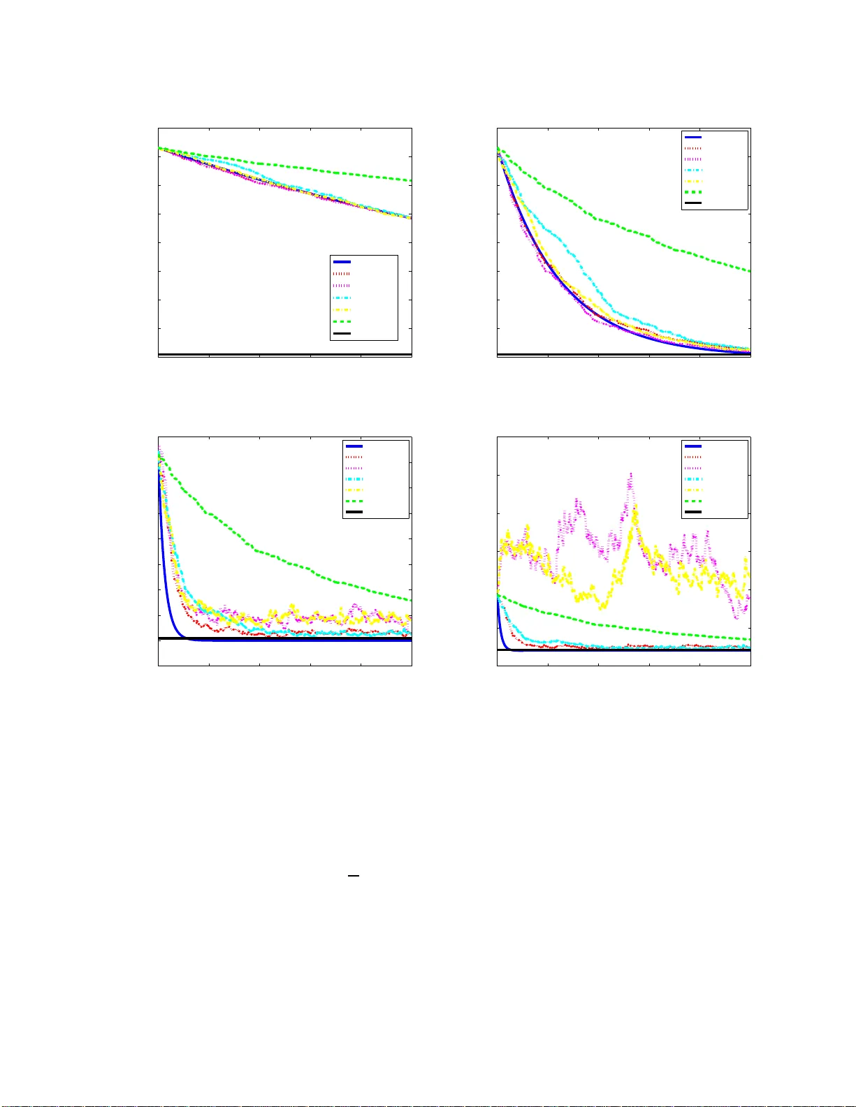
Online and sto c hastic Douglas-Rac hford splitti ng metho d for large scale mac hine learning Ziqiang Shi ∗ † , Rujie Liu ∗ August 7, 2018 Abstract Online and stochastic learning has emerged as pow erful to ol in large scale optimization. In this wo rk , w e generalize the Douglas-Rac h ford splitting (DR s) met h od for minimizing composite functions to online and stochastic settings (to our b est knowle dge this is the first time DRs b een generalized to sequential versi on ) . W e fi rst establish an O (1 / √ T ) regret b ound for batch D R s metho d. Then we p ro ved that the online DR s splitting meth o d enjoy an O (1) regret b ound and sto chas t ic DRs splitting has a con vergence rate of O (1 / √ T ). The pro of is simple and in tuitive, and the results and tec hniq ue can be serve d as a initiate for the research on the large scale mac hine learning employ the DRs meth od. Numerical exp eriments of t he prop osed met h od demonstrate th e effective n ess of th e online and stochastic up date rule, and further confirm our regret and conv ergence analysis. 1 In tro d uction and problem statemen t First introduced in [4 ], the Doug las-Rachford splitting technique has beco me p opular in r e cent years due to its fa s t theoretical conv ergence rate and str ong practica l per formance. The metho d is first pro p o sed to addresses the minimization of the sum of t wo functions g ( x )+ h ( x ). It was extended in [11] to handle pro blems inv olving the sum of tw o no nlinear monotone op erator problems. F or further developments, see [7, 2, 3]. How ever, most of these v ariants implicitly ass ume full accessibility of all data v alues, while in r eality one can hardly ignore the fac t that the size of data is r apidly increasing in v ario us domain, and thus batch mo de learning pr o cedure ca nnot deal with the h uge size training set for the data pro ba bly cannot be loaded into the memory simult a neously . F urthermore, it cannot be star ted un til the tra ining da ta is pr epared, hence cannot effectively dea l with tra ining data appea r in s equence, suc h as audio and video pro cess ing [15]. In such situatio n, seq ue ntial learning b ecome p ow erful to ols. Online a nd sto chastic learning ar e of the most pro mising metho ds in lar ge scale machine learning tasks in these days [2 0, 18]. Imp ortant adv ances ha ve been made on sequential le a rning in the r ecent liter ature on simila r problems. Compo site ob jective mirror desce nt (COMID) [5] genera lizes mirror descent [1] to the online s e tting. Regularized dua l averaging (RDA ) [1 9] gener alizes dual av er aging [13] to online and comp osite optimization, and can b e used for distributed optimization [6]. Online alterna ting direction mul- tiplier metho d (ADMM) [16], RD A-ADMM [16] and online proximal gra dient (O PG) ADMM [18] g eneralize classical ADMM [8] to o nline and sto chastic settings . Our fo cus in this pa p er is to genera liz e the Douglas- Ra chf ord splitting to online and s to chastic settings. In this work, we consider the problems of the following form: minimize x ∈ R n f T ( x ) := 1 T T X t =1 g t ( x ) + h ( x ) = 1 T T X t =1 ( g t ( x ) + h ( x )) , (1.1) where g t is a conv ex loss function asso c ia ted with a sample in a training set, and h is a no n-smo oth c onv ex pena lty function or regula rizer. Many pr oblems o f relev ance in signa l pro cess ing and machine lear ning can be ∗ F ujitsu Research & Developmen t Cen ter, Beijing, China. † shiziqiang@cn.fujitsu.com 1 formulated as the a b ove optimization proble m. Similar problems include the r idge regr ession, the lasso [1 7 ], the logistic reg ression, a nd the minimization of total v ar iation. Let g ( x ) = 1 T P T t =1 g t ( x ) in Pr oblem (1.1), and then the Douglas-Rachford splitting a lgorithm approxi- mates a minimizer o f (1 .1) with the help of the following sequence: u t +1 = u t + λ t { prox λg [2 prox λh ( u t ) − u t ] − pr ox λh ( u t ) } , where ( λ t ) t ≥ 0 ⊂ [0 , 2] satisfies P t ≥ 1 λ t (2 − λ t ) = ∞ , and the pr oximal mapping of a c onv ex function h at x is prox h ( t ) := arg min y ∈ R n h ( y ) + 1 2 k y − t k 2 . Thu s the itera tive scheme of Douglas-Rachford splitting for the pr oblem (1.1) is as follows: x t +1 = arg min x h ( x ) + 1 2 λ k x − u t k 2 , (1.2) z t +1 = arg min z g ( z ) + 1 2 λ k z − (2 x t +1 − u t ) k 2 , (1.3) u t +1 = u t + λ t ( z t +1 − x t +1 ) , (1.4) where ( u t ) t ∈ N conv erg es weakly (in Hilb ert s pace R n , weak convergence is equiv alent to s trong conv er gence) to some p o int u (th us also x t , for prox λh ( · ) is contin uous), and prox λh ( u ) is a so lution to Pr oblem (1 .1). F o r conv enience of description, we assume a ll λ t = 1 in this work. The only mo dification of the s plitting that we pro po se for o nline and sto chastic pro c essing is s imple: z t +1 = ar g min z g t ( z ) + 1 2 λ k z − (2 x t +1 − u t ) k 2 , and z t +1 = ar g min z g i t ( z ) + 1 2 λ k z − (2 x t +1 − u t ) k 2 , where index i t is sampled uniformly from the set { 1 , ..., T } W e call these metho ds online DRs (o DRs) and sto chastic DRs (sDRs) resp ectively . Due to the complex lo ss function g t ( z ), gener ally the up date is difficult to solve efficiently . A common wa y is to linearize the ob jective such that z t +1 = ar g min z ∇ g t ( z t ) T ( z − z t ) + 1 2 λ k z − (2 x t +1 − u t ) k 2 , (1.5) and z t +1 = ar g min z ∇ g i t ( z t ) T ( z − z t ) + 1 2 λ k z − (2 x t +1 − u t ) k 2 , which ar e ca lled inexact oDRs (ioDRs) and inexact sDRs (isDRs) r esp ectively . ioDRs o r isDRs ca n also b e derived from a nother po int o f view, which is ba sed o n pr oximal gr adient [12]. Here we use ioDRs as an example. The proximal gr adient metho d uses the proximal mapping of the nonsmo oth par t to minimize c omp o site functions (1.1) [1 0]: x t +1 = prox λ t h ( x t − λ t ∇ g ( x t )) = ar g min y ∇ g ( x t ) T ( y − x t ) + 1 2 λ t k y − x t k 2 + h ( y ) , where λ t denotes the t -th step length. Then the online P G (OP G) is straight forward, tha t is at around t solving the following optimiza tion problem with the lineariza tion of only t -th lo ss function g t ( x ) [19, 6, 16]: x t +1 = ar g min y ∇ g t ( x t ) T ( y − x t ) + 1 2 λ t k y − x t k 2 + h ( y ) . Then the ioDRs ca n b e seen as a combination of O PG with DRs. 2 2 Con v ergence Analysis for DRs The pro cedure of ba tch DRs is summarized in Algotihtm 1. It is c le a r that x ∗ is a so lution o f Pr oblem (1.1) if and only if 0 ∈ ∂ g ( x ∗ ) + ∂ h ( x ∗ ), whic h is equiv alent to x ∗ − λ∂ g ( x ∗ ) ∈ x ∗ + λ∂ h ( x ∗ ), where λ > 0. It is clear that ∂ g ( x ) and ∂ h ( x ) are tw o monotone set-v alued o p e r ators [14], and the r esolven t op era tors R λ ∂ g := ( I + λ∂ g ) − 1 and R λ ∂ h := ( I + λ∂ h ) − 1 are b oth single v a lued. Thus if the lo ss functions g t are smo oth, we hav e x ∗ = R λ ∂ h ( x ∗ − λ ∇ g ( x ∗ )), which immediately g ives an accuracy mea sure prop o s ed in [9] of a vector x to a solution of P roblem (1.1) by ε g ( x, λ ) = x − R λ ∂ h ( x − λ ∇ g ( x )) . After t iterations of (1.2), fro m ε = x t − R λ ∂ h ( x t − λ ∇ g ( x t )), w e ha ve ε λ ∈ ∇ g ( x t ) + ∂ h ( x t − ε ). Since g ( x ) a nd f ( x ) are conv ex functions, using their (sub)gradients, we hav e g ( x t ) − g ( x ∗ ) ≤ h x t − x ∗ , ∇ g ( x t ) i (2.1) h ( x t − ε ) − h ( x ∗ ) ≤ h x t − ε − x ∗ , ph ( x t − ε ) i , (2.2) h ( x t ) − h ( x t − ε ) ≤ h ε, ph ( x t ) i , (2.3) where ph ( x t − ε ) ∈ ∂ h ( x t − ε ) is the subg radient of h ( x ) at x t − ε satisfying ε λ = ∇ g ( x t ) + ph ( x t − ε ), and ph ( x t ) ∈ ∂ h ( x t ) is any subgra dient of h ( x ) at x t . Adding (2.1), (2.2), and (2 .3) together yields g ( x t ) + h ( x t ) − ( g ( x ∗ ) + h ( x ∗ )) ≤h x t − x ∗ , ∇ g ( x t ) + ph ( x t − ε ) i + h ε, ph ( x t ) − ph ( x t − ε ) i , (2.4) ≤h x t − x ∗ , ε λ i + h ε, ph ( x t ) − ph ( x t − ε ) i . If h ( x ) is Lipschitz contin uous with Lips chit z constant L h , then we hav e k ph ( x ) k ≤ L h , w he r e ph ( x ) is any subgradient of h ( x ) at x . F ur thermore x t is b ounded for its convergence. Thus we ha ve k ph ( x t ) − ph ( x t − ε ) k = O (1), k x t − x ∗ k = O (1), th us the following conv erg ence result holds. Theorem 2.1. Assu me g ( x ) is differ entiable, h ( x ) is Lipsch itz c ont inu ous. L et the se quenc e { x t , z t , u t } b e gener ate d by DRs. Then we have g ( x T ) + h ( x T ) − ( g ( x ∗ ) + h ( x ∗ )) = O ( ε g ( x T , λ )) . R emark 1 . F rom above theorem, we no tice that if we have a fa s ter conv erg ent rate o f ε g ( x T , λ ), then we hav e a faster conv er gent rate of the optimizing v alue. It is sho wed in Theorem 3.1 of [9] that after t iterations of (1.2), we have k ε g ( x t , λ ) k 2 = O (1 / t ) . Thu s we hav e Corollary 2.2. Assume g ( x ) is differ entiable, h ( x ) is Lipschitz c ontinuous. L et the se quenc e { x t , z t , u t } b e gener ate d by DRs in Algotihtm 1. Then we have g ( x T ) + h ( x T ) − ( g ( x ∗ ) + h ( x ∗ )) = O (1 / √ T ) . R emark 2 . If g ( x ) is Lipschitz contin uous with Lipschitz cons ta nt L g and the set of all ∂ h ( x ) is b ounded b y some constant N ∂ h , then we ca n obta in an explicit b ound by using Lemma 3.1 of [9], which shows us that k ( x t − x ∗ ) + λ ( ∇ g ( x t ) − ∇ g ( x ∗ )) k is monotonically decrea sing. Th us we hav e k x t − x ∗ k ≤ k x 0 − x ∗ k + 4 λL g from the following inferenc e k x t − x ∗ k − 2 λL g ≤k ( x t − x ∗ ) + λ ( ∇ g ( x t ) − ∇ g ( x ∗ )) k ≤k ( x 0 − x ∗ ) + λ ( ∇ g ( x 0 ) − ∇ g ( x ∗ )) k (2.5) ≤k x 0 − x ∗ k + 2 λL g . 3 F urther fro m Theo rem 3.1 in [9], we have k ε g ( x t , λ ) k ≤ 1 √ t + 1 k ( x t − x ∗ ) + λ ( ∇ g ( x t ) − ∇ g ( x ∗ )) k ≤ 1 √ t + 1 ( k x t − x ∗ k + 2 λL g ) ≤ 1 √ t + 1 ( k x 0 − x ∗ k + 6 λL g ) . Then accor ding to (2.4), w e have g ( x T ) + h ( x T ) − ( g ( x ∗ ) + h ( x ∗ )) ≤h x T − x ∗ , ε λ i + h ε, ph ( x T ) − ph ( x T − ε ) i ≤k x T − x ∗ kk ε λ k + k ε k k ph ( x T ) − ph ( x T − ε ) ik (2.6) ≤ 1 λ ( k x 0 − x ∗ k + 4 λL g ) k ε k + 2 N ∂ h k ε k . Thu s we hav e the following corollar y . Corollary 2.3. As sume g ( x ) is differ entiable, b oth h ( x ) and g ( x ) ar e Lipsch itz c ontinuous, and the set of al l ∂ h ( x ) is b ounde d by some c onstant N ∂ h . L et the se qu enc e { x t , z t , u t } b e gener ate d by DRs. Then we have g ( x T ) + h ( x T ) − ( g ( x ∗ ) + h ( x ∗ )) ≤ 1 λ √ T + 1 ( k x 0 − x ∗ k + 4 λL g )( k x 0 − x ∗ k + 6 λL g ) + 2 N ∂ h √ T + 1 ( k x 0 − x ∗ k + 6 λL g ) . R emark 3 . If further more ∇ g ( x ) is Lipschitz contin uous with L ∇ g , then fro m (2 .5 ) w e have k x t − x ∗ k ≤ 1+ λL ∇ g 1 − λL ∇ g k x 0 − x ∗ k from the following der iv ation (1 − λL ∇ g ) k x t − x ∗ k ≤k ( x t − x ∗ ) + λ ( ∇ g ( x t ) − ∇ g ( x ∗ )) k ≤k ( x 0 − x ∗ ) + λ ( ∇ g ( x 0 ) − ∇ g ( x ∗ )) k (2.7) ≤ (1 + λL ∇ g ) k x 0 − x ∗ k . Then due to the simila r for mulation, w e hav e k ε g ( x t , λ ) k ≤ 1+ λL ∇ g √ t +1 k x 0 − x ∗ k . Put these new inequalities int o (2.6), then we hav e the following r ate. Corollary 2. 4. Assume g ( x ) is differ entiable, b oth h ( x ) and g ( x ) ar e Lipschitz c ont inu ous, the set of al l ∂ h ( x ) is b ounde d by some c onstant N ∂ h , and ∇ g ( x ) is Lipschitz c ontinuous with L ∇ g . L et the se quenc e { x t , z t , u t } b e gener ate d by DRs. Then we have g ( x T ) + h ( x T ) − ( g ( x ∗ ) + h ( x ∗ )) ≤ ( (1 + λL ∇ g ) λ (1 − λL ∇ g ) + 2 N ∂ h ) 1 + λL ∇ g √ T + 1 k x 0 − x ∗ k . These above results are all base d and derived fr om the for mulation of [9], we wonder what we can obtain from the DR itera tion formulations (1.2), (1.3), and (1.4 ). F ro m (1.2 ), we hav e 0 ∈ ∂ h ( x t +1 ) + 1 λ ( x t +1 − u t ) ⇒ − 1 λ ( x t +1 − u t ) ∈ ∂ h ( x t +1 ) . (2.8) 4 Algorithm 1 A g e ne r ic DRs Input : starting p oint x 0 ∈ dom( g + h ). 1: for t = 0 , 1 , · · · , T do 2: x t +1 = arg min x h ( x ) + 1 2 λ k x − u t k 2 . 3: z t +1 = arg min z g t +1 ( z ) + 1 2 λ k z − (2 x t +1 − u t ) k 2 . 4: u t +1 = u t + λ t ( z t +1 − x t +1 ). 5: en d for Output : x T +1 . F rom (1.3), we have 0 ∈ ∂ g ( z t +1 ) + 1 λ ( z t +1 − (2 x t +1 − u t )) ⇒ − 1 λ ( z t +1 − (2 x t +1 − u t )) ∈ ∂ g ( z t +1 ) . Using (1.4) yields − 1 λ ( u t +1 − x t +1 ) ∈ ∂ g ( z t +1 ) . (2.9) Since h and g are co nv ex functions and their subgradients ar e given in (2.8) a nd (2.9) resp ectively , we have, h ( x t +1 ) − h ( x ∗ ) ≤h− 1 λ ( x t +1 − u t ) , x t +1 − x ∗ i , g ( z t +1 ) − g ( x ∗ ) ≤h− 1 λ ( u t +1 − x t +1 ) , z t +1 − x ∗ i Adding ab ov e toge ther yields h ( x t +1 ) + g ( z t +1 ) − ( h ( x ∗ ) + g ( x ∗ )) ≤h− 1 λ ( x t +1 − u t ) , x t +1 − x ∗ i + h− 1 λ ( u t +1 − x t +1 ) , z t +1 − x ∗ i (2.10) = 1 λ [ u t +1 ( x ∗ − z t +1 ) + x t +1 ( z t +1 − x t +1 ) + u t ( x t +1 − x ∗ )] If g ( x ) is Lipschitz contin uous with Lipschitz consta n t L g , then we have k g ( x t +1 ) − g ( z t +1 ) k ≤ L g k x t +1 − z t +1 k , adding with (2.1 0) yields h ( x t +1 ) + g ( x t +1 ) − ( h ( x ∗ ) + g ( x ∗ )) ≤ 1 λ [ u t +1 ( x ∗ − z t +1 ) + u t ( x t +1 − x ∗ )] + ( L g + 1 λ k x t +1 k ) k x t +1 − z t +1 k . Thu s we hav e Theorem 2.5 . Assu me g ( x ) is Lipschitz c ontinu ous. L et t he se qu en c e { x t , z t , u t } b e gener ate d by DR s. Then we have g ( x T ) + h ( x T ) − ( g ( x ∗ ) + h ( x ∗ )) = O ( x T − x ∗ ) . 3 Online and sto c hastic Douglas-Rac hford splitting metho d In this se c tion, w e generalize the DRs to online and sto chastic settings. The pro c e dure of ba tch DRs, oDRs, ioDRs, sDRs, and isDRs ar e summar ized in Algo tih tm 1, 2, 3, 4 a nd 5 r esp ectively , where f 1 ( x ) = g 1 ( x ) + h ( x ). 5 Algorithm 2 A g e ne r ic oDRs Input : starting p oint x 0 ∈ dom f 1 . 1: for t = 0 , · · · , T do 2: x t +1 = arg min x h ( x ) + 1 2 λ k x − u t k 2 . 3: z t +1 = arg min z g t +1 ( z ) + 1 2 λ k z − (2 x t +1 − u t ) k 2 . 4: u t +1 = u t + λ t ( z t +1 − x t +1 ). 5: en d for Output : x T +1 . Algorithm 3 A g e ne r ic ioDRs Input : starting p oint x 0 ∈ dom f 1 . 1: for t = 0 , · · · , T do 2: x t +1 = arg min x h ( x ) + 1 2 λ k x − u t k 2 . 3: z t +1 = arg min z ∇ g t +1 ( z t ) T ( z − z t ) + 1 2 λ k z − (2 x t +1 − u t ) k 2 . 4: u t +1 = u t + λ t ( z t +1 − x t +1 ). 5: en d for Output : x T +1 . 3.1 Regret Analysis for oDRs The goa l of oDRs is to a chieve low regre t w.r.t. a static predictor o n a sequence of functions f T ( x ) = 1 T T X t =1 g t ( x ) + h ( x ) . According to Algotihtm 2, for mally , a t every ro und o f the algor ithm we ma ke a pr ediction x t and then receive the function f t ( x ) = g t ( x ) + h ( x ). That is at r ound t − 1, we o btain x t by solv ing the following problem: x ∗ t = ar g min x g t ( x ) + h ( x ) with only single DR iter ation based on the warm start x t − 1 . In ba tch optimization we se t f t = f for all t while in sto chastic optimization we choose f t to b e the average of some random subset of { f 1 , ..., f T } . In this work, w e seek bounds on the s tandard r egret in the online learning s etting with res pec t to x ∗ , defined as R ( T , x ∗ ) := 1 T T X t =1 ( g t ( x t ) + h ( x t )) − [ 1 T T X t =1 g t ( x ∗ ) + h ( x ∗ )] As p ointed b y (2.7) a nd Theore m 3.1 in [9], with the notation ε g t ( x t , λ ) = x t − R λ ∂ h ( x t − λ ∇ g t ( x t )) in mind, we have in each iteration that k x t − x ∗ t k ≤ 1 + λL ∇ g t 1 − λL ∇ g t k x t − 1 − x ∗ t k and k ε g t ( x t , λ ) k 2 ≤ 1 2 k ( x t − 1 − x ∗ t ) + λ ( ∇ g t ( x t − 1 ) − ∇ g t ( x ∗ t )) k 2 , which means that O (1) λ ∈ ∇ g t ( x t ) + ∂ h ( x t − O (1)) . F ollowing the s ame pro cedure as (2.4), we have g t ( x t ) + h ( x t ) − ( g t ( x ∗ ) + h ( x ∗ )) ≤h x t − x ∗ , O (1) λ i + h O (1) , ph ( x t ) − ph ( x t − O (1)) i = O (1) . Summing up ab ov e for m ula s for t ∈ { 1 , ..., T } , we obtain the following result: 6 Algorithm 4 A g e ne r ic sDRs Input : starting p oint x 0 ∈ dom f 1 . 1: for t = 0 , · · · , T do 2: x t +1 = arg min x h ( x ) + 1 2 λ k x − u t k 2 . 3: Ra ndomly select index i t from the set { 1 , ..., T } and s olve the subpro blem: z t +1 = arg min z g i t +1 ( z ) + 1 2 λ k z − (2 x t +1 − u t ) k 2 . 4: u t +1 = u t + λ t ( z t +1 − x t +1 ). 5: en d for Output : x T +1 . Algorithm 5 A g e ne r ic ioDRs Input : starting p oint x 0 ∈ dom f 1 . 1: for t = 0 , · · · , T do 2: x t +1 = arg min x h ( x ) + 1 2 λ k x − u t k 2 . 3: Ra ndomly select index i t from the set { 1 , ..., T } and s olve the subpro blem: z t +1 = ar g min z ∇ g i t +1 ( z t ) T ( z − z t ) + 1 2 λ k z − (2 x t +1 − u t ) k 2 . 4: u t +1 = u t + λ t ( z t +1 − x t +1 ). 5: en d for Output : x T +1 . Theorem 3 .1. A s sume al l g t ( x ) ar e differ entiable, h ( x ) and g t ( x ) ar e Lipsch itz c ontinuous, the set of al l ∂ h ( x ) is b ounde d by some c onstant N ∂ h , ∇ g t ( x ) is Lipschitz c ontinu ous with L ∇ g t , al l L ∇ g t and x ∗ t ar e b ounde d. L et the se quenc e { x t , z t , u t } b e gener ate d by oDRs. Then we have R ( T , x ∗ ) = O (1) . 3.2 Con ve rgence analysis of sDR s F rom (2.7) and Theor em 3.1 in [9], we hav e in ea ch iter ation of Algotihtm 4 that k x t − x ∗ t k ≤ 1 + λL ∇ g i t 1 − λL ∇ g i t k x t − 1 − x ∗ t k and k ε g i t ( x t , λ ) k 2 ≤ 1 2 k ( x t − 1 − x ∗ t ) + λ ( ∇ g i t ( x t − 1 ) − ∇ g i t ( x ∗ t )) k 2 , which means that O (1) λ ∈ ∇ g i t ( x t ) + ∂ h ( x t − O (1)) . F ollowing the s ame pro cedure as (2.4), we have g i t ( x t ) + h ( x t ) − ( g i t ( x ∗ ) + h ( x ∗ )) ≤h x t − x ∗ , O (1) λ i + h O (1) , ph ( x t ) − ph ( x t − O (1)) i = O (1) . Thu s we obtain the following result: 7 Theorem 3 .2. A s sume al l g t ( x ) ar e differ entiable, h ( x ) and g t ( x ) ar e Lipsch itz c ontinuous, the set of al l ∂ h ( x ) is b ounde d by some c onstant N ∂ h , ∇ g t ( x ) is Lipschitz c ontinu ous with L ∇ g t , al l L ∇ g t and x ∗ t ar e b ounde d. L et the se quenc e { x t , z t , u t } b e gener ate d by Algotih t m 4. Then we have g ( x T ) + h ( x T ) − ( g ( x ∗ ) + h ( x ∗ )) = O (1 / √ T ) . 4 Computational exp erimen ts In this sectio n, w e demonstrate the p er fo rmance of oDRs and s DRs in solv ing se veral machine learning problems. W e present s imulation results to show the c onv erge nc e of the ob jective in oDRs a nd sDRs. W e also co mpa re them with batch DRs and O ADM [18]. W e set λ t = 1 for all the updates of u t +1 , and λ = [0 . 1 , 1 , 10 , 20]. All the ex per iments show that o DRs and sDRs o utper form OAD M. 4.1 Lasso The lasso problem is for mulated as follows: minimize x ∈ R n × 1 1 T T X t =1 k a T t x − b t k 2 + µ k x k 1 , (4.1) where a t , x ∈ R n × 1 and b t is a scala r. The three upda tas of DRs are : x t +1 = arg min x µ k x k 1 + 1 2 λ k x − u t k 2 = sign( u t ) · max { | u t | − µλ, 0 } , z t +1 = arg min z 1 T T X t =1 k a T t z − b t k 2 + 1 2 λ k z − (2 x t +1 − u t ) k 2 =( A T A + T 2 λ I ) − 1 [ A T b + T 2 λ (2 x t +1 − u t )] , u t +1 = u t + λ t ( z t +1 − x t +1 ) , where A = ( a 1 , ..., a T ) and b = ( b 1 , ..., b T ) T . The difference s of oDRs and ioDRs from DRs is the update of z t +1 , which a r e: z t +1 = arg min z k a T t z − b t k 2 + 1 2 λ k z − (2 x t +1 − t t ) k 2 = [ a T t a t + 1 2 λ I ] − 1 [ a t b t + 1 2 λ (2 x t +1 − u t )] and z t +1 = ar g min z 2( a T t z t − b t ) a T t ( z − z t ) + 1 2 λ k z − (2 x t +1 − u t ) k 2 = 2 x t +1 − u t − 2 λ ( a T t z t − b t ) a t resp ectively . Our exp eriments mainly follow the lass o example in [18]. W e firs t randomly g enerated A with 1000 examples of dimensio nality 100. A is then nor malized along the columns. Then, a true x 0 is randomly generated with certain spars it y pattern for lasso, and we set the n umber of nonzer os as 1 0. b is calculated by adding Gaussia n no ise to Ax 0 /T , where T = 1000 is n umber of ex amples. W e set µ = 0 . 1 × k A T b/T k ∞ and η = 1 in OADM [1 8]. All exp eriments a re implemen ted in Matlab. In Figur e 1, the ob jective v alue of the problem is depicted a gainst the iter ation times. In this example, oDRs and sDRs show faster conv erge nce tha n OADM, io DRs, and isDRs. The ma in reaso n for the slow conv erg ence of ioDRs or isDRs is b ecaus e the linear ization of the ob jective in each iteration (1.5). W e observe that OADM ta kes even longer itera tions to achiev e a certa in precisio n, although the reg ret b ound is more tighter than the b ound obtained in this work for oDRs ( O (1 / √ T ) in OADM [18], while O (1) in o DRs). Thu s we b elieve and conjecture that the regr et R ( T , x ∗ ) in Theorem 3.1 is indeed O (1 / √ T ). 8 0 200 400 600 800 1000 2 3 4 5 6 7 8 9 10 x 10 −3 iter (k) f(x k ) + g(x k ) DRs oDRs ioDRs sDRs isDRs OADMM True value (a) λ =0.1 0 200 400 600 800 1000 2 3 4 5 6 7 8 9 10 x 10 −3 iter (k) f(x k ) + g(x k ) DRs oDRs ioDRs sDRs isDRs OADMM True value (b) λ =1 0 200 400 600 800 1000 1 2 3 4 5 6 7 8 9 10 x 10 −3 iter (k) f(x k ) + g(x k ) DRs oDRs ioDRs sDRs isDRs OADMM True value (c) λ =10 0 200 400 600 800 1000 0 0.005 0.01 0.015 0.02 0.025 0.03 iter (k) f(x k ) + g(x k ) DRs oDRs ioDRs sDRs isDRs OADMM True value (d) λ =20 Figure 1 : The co nv ergence of ob jective v alue in DRs, oDRs, ioDRs, s DRs, isDRs, OADM, and real ob jective v alue for the lass o pro blem (4.1). 4.2 Logistic regression The logistic reg ression pr oblem is formulated a s follows: minimize w ∈ R n 1 T T X i =1 log(1 + exp( − y i w T x i )) + µ k w k 1 , (4.2) where x (1) , . . . , x ( T ) are samples with lab els y (1) , . . . , y ( T ) ∈ { 0 , 1 } , the regularizatio n term k w k 1 promotes sparse solutio ns and µ balances g o o dness-of-fit and spar sity . 9 The three up datas of DRs a re: w t +1 = ar g min w µ k w k 1 + 1 2 λ k w − u t k 2 = sign( w t ) · max { | w t | − µλ, 0 } , z t +1 = ar g min z 1 T T X i =1 log(1 + e xp( − y i z T x i )) + 1 2 λ k z − (2 w t +1 − u t ) k 2 , u t +1 = u t + λ t ( z t +1 − x t +1 ) . The differences of oDRs and ioDRs from DRs is the up date of z t +1 , which are: z t +1 = ar g min z log(1 + exp( − y t z T x t )) + 1 2 λ k z − (2 w t +1 − u t ) k 2 , and z t +1 = ar g min z − 1 + exp( − y t z T t x t ) exp( − y t z T t x t ) y t x t ( z − z t ) + 1 2 λ k z − (2 w t +1 − u t ) k 2 . The sDRs and isDRs a re almost the same, we will no t r ep eat here. 4.3 T otal v ariation minimization The total v ariation (TV) minimization problem is formulated as follows: minimize x ∈ R n × 1 1 T T X t =1 k a T t x − b t k 2 + µ T − 1 X t =1 k x t +1 − x t k 1 , (4.3) where a t , x ∈ R n × 1 and b t is a scala r. The three up datas of DRs a re: x t +1 = ar g min x µ k Dx k 1 + 1 2 λ k x − u t k 2 = ar g min x µ k Dx k 1 + 1 2 λ k E D x − E D u t k 2 , z t +1 = ar g min z 1 T T X t =1 k a T t z − b t k 2 + 1 2 λ k z − (2 x t +1 − u t ) k 2 = ( A T A + T 2 λ I ) − 1 [ A T b + T 2 λ (2 x t +1 − u t )] , u t +1 = u t + λ t ( z t +1 − x t +1 ) , where A = ( a 1 , ..., a T ), b = ( b 1 , ..., b T ) T and D is an upp er bi-diagona l matr ix with diag onal 1 and o ff- diagonal -1, and E D = I . Here we s hould no tice that the up date of x is obta ined by solving a sma ll scale lasso problem. Here we employ the DR algor ithm to s olve it. The difference s o f oDRs and io DRs from DRs is the up date of z t +1 , which a r e: z t +1 = arg min z k a T t z − b t k 2 + 1 2 λ k z − (2 x t +1 − t t ) k 2 = [ a T t a t + 1 2 λ I ] − 1 [ a t b t + 1 2 λ (2 x t +1 − u t )] and z t +1 = ar g min z 2( a T t z t − b t ) a T t ( z − z t ) + 1 2 λ k z − (2 x t +1 − u t ) k 2 = 2 x t +1 − u t − 2 λ ( a T t z t − b t ) a t resp ectively . Based on the numerical tes ts , we prop ose the following tw o very credible conjectures: 10 Conjecture 4. 1. Assu me g ( x ) is differ entiable, h ( x ) is Lipschitz c ontinuous. L et the se quenc e { x t , z t , u t } b e gener ate d by ioDRs. Then we have R ( T , x ∗ ) = O (1) . and Conjecture 4. 2. Assu me g ( x ) is differ entiable, h ( x ) is Lipschitz c ontinuous. L et the se quenc e { x t , z t , u t } b e gener ate d by isDRs. Then we have g ( x T ) + h ( x T ) − ( g ( x ∗ ) + h ( x ∗ )) = O (1 / √ T ) . 5 Conclusion In this pap er , we prop ose the efficient online and sto chastic learning algo rithm na med online DRs (oDRs) and stochastic DRs (sDRs) r esp ectively . New proo f techniques hav e been developed to analyze the reg ret of DRs, o DRs a nd co nv ergence of sDRs, which shows that DRs and oDRs hav e O (1 / √ T ) and O (1) reg ret resp ectively , a nd sDRs enjoys a conv erg ence rate of O (1 / √ T ). Finally , we illustra te the efficiency of oDRs and sDRs in solving s e veral machine learning problems. References [1] Amir Beck a nd Ma r c T eb oulle. Mirror des cent a nd nonlinea r pro jected subgradient metho ds for conv ex optimization. Op er ations R ese ar ch L etters , 31(3):167 –175 , 2003 . [2] Patric k L Co m b ettes. I ter ative construction of the resolven t o f a sum of maximal monotone op erator s. J. Convex Anal , 16(4):7 2 7–74 8, 200 9. [3] Patric k L Com b ettes and Jean-Christo phe Pesquet. Pro ximal splitting metho ds in signal pro cessing. In Fixe d-Point Algorithms for Inverse Pr oblems in Scienc e and Engine ering , pag es 185 –212 . Spring er, 2011. [4] Jim Doug las and HH Rachford. On the numerical solution of heat conduction pro blems in tw o and three space v ariables. T r ansactions of the Americ an mathematic al So ciety , 82(2):42 1–43 9, 1 956. [5] John Duchi, Shai Shalev-Shw ar tz, Y or am Singer, and Am buj T ewari. Co mpo site ob jective mir ror de- scent. 2 010. [6] John C Duchi, Alekh Agar wal, and Martin J W ainwright. Dual av era ging for distributed optimization. In Co mm unic ation, Contr ol, and Computing (Al lerton), 2012 50 t h Annual Al lerton Confer enc e on , pages 156 4–156 5. IEE E, 2 012. [7] Jonathan E ckstein a nd Dimitri P Ber tsek as. On the douglasr achford splitting metho d and the proximal po int algo rithm for maxima l monotone op erator s. Mathematic al Pr o gr amming , 5 5(1-3):29 3–31 8 , 199 2. [8] Daniel Gabay and Bertr a nd Mercier. A dua l algo rithm for the so lution of nonlinear v ariatio nal problems via finite element appr oximation. Computers & Mathematics with Applic ations , 2(1):17 –40, 197 6. [9] BS He and XM Y ua n. On conv ergence rate of the dougla s-rachford ope r ator splitting metho d. Mathe- matic al Pr o gr amming, under r evision , 2011 . [10] Jaso n D Lee, Y uek ai Sun, and Michael A Saunder s. Pr oximal newton- t y pe metho ds for minimizing comp osite functions. 2 013. [11] Pierr e-Louis Lions and Bertra nd Mercier . Splitting algor ithms for the s um of tw o nonlinear o p e rators. SIAM Journal on Nu meric al Analysis , 16(6):964 –979, 19 7 9. [12] Y urii Nesterov. Gradient metho ds for minimizing compo site ob jective function, 2 007. 11 [13] Y urii Nesterov. Primal- dual subgra dient metho ds for conv ex pr oblems. Mathematic al pr o gr amming , 120(1):22 1–25 9, 200 9. [14] R Tyrell Ro ck afellar. Convex analysis , volume 28. Princeton university pr ess, 1997 . [15] Ziqiang Shi, J iq ing Han, Tieran Zheng, and Shiwen Deng . Audio se gment class ific a tion using online learning base d tensor re pr esentation featur e discriminatio n. IEEE tr ansactions on audio, sp e e ch, and language pr o c essing , 21(1-2 ):186–1 9 6, 20 13. [16] T aiji Suzuki. Dual averaging and pr oximal gra dient des cent for online alternating direction multiplier metho d. In Pr o c e e dings of the 30th International Confer enc e on Machine L e arning (ICML-13 ) , pa g es 392–4 00, 2013 . [17] Rob ert Tibshirani. Regr e ssion shr ink age and selection via the lasso. Journal of the Ro yal Statistic al So ciety. Series B (Metho dolo gic al) , pages 267– 288, 199 6 . [18] Huahua W ang and Arindam Baner jee. Online alter nating direction metho d. arXiv pr eprint arXiv:120 6.6448 , 2012. [19] Lin Xiao. Dual av er aging metho ds for regular ized sto chastic learning and online optimization. The Journal of Machine L e arning R ese ar ch , 11:254 3–25 9 6, 2010 . [20] Martin Zinkevic h. Online conv e x prog ramming and g eneralized infinitesimal gra dient a s cent. 2003 . 12 0 200 400 600 800 1000 2 3 4 5 6 7 8 9 10 x 10 −3 iter (k) f(x k ) + g(x k ) DRs oDRs ioDRs sDRs isDRs OADMM True value