Sufficient Conditions for Recognizing a 3-manifold Group

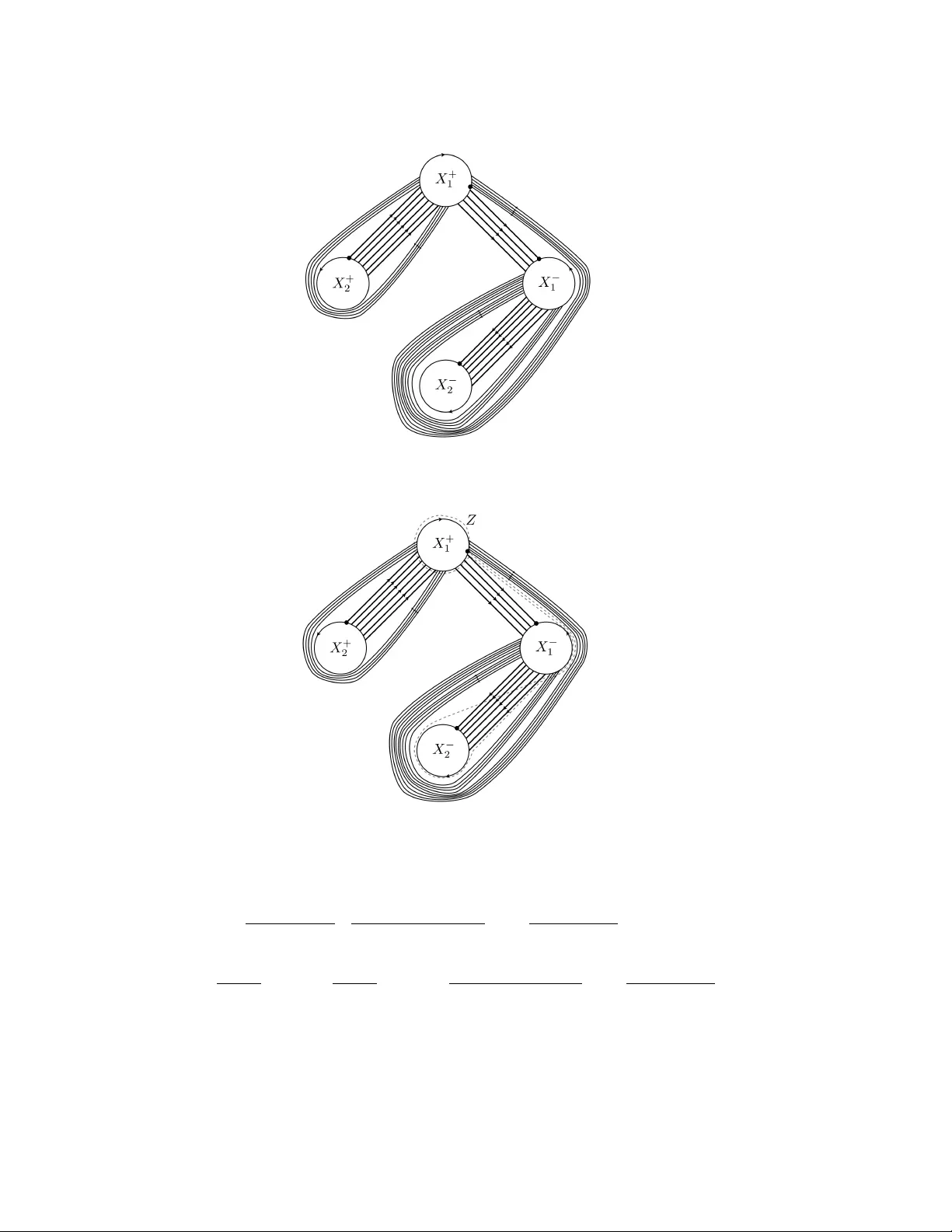
SUFFICIENT CONDITIONS F OR RECOGNIZING A 3-MANIF OLD GR OUP KAR OLINE NULL Abstract. In this w ork we ask when a group is a 3-manifold group, or more sp ecifically , when do es a group presen tation come naturally from a Heegaard diagram for a 3-manifold? W e will give some conditions for partial answ ers to this form of the Isomorphism Problem b y addressing ho w the presentation asso ciated to a diagram for a splitting is related to the fundamen tal group of a 3-manifold. In the pro cess, w e determine an in v arian t of groups (b y w ay of group presentations) for how far such presentations are from 3-manifolds. 1. Introduction Mathematicians first became interested in 3-manifolds ov er 100 y ears ago, with the writings of Henri Poincare and the contin ued w ork of Poul Heegaard. Despite the passage of time and the atten tion giv en to them, 3-manifolds remain a very activ e and in triguing field for the simplest of reasons. W e still cannot answ er the most basic questions about them: given 3-manifolds M 1 and M 2 , is M 1 ' M 2 (the Home omorphism Pr oblem )? Or, is π 1 ( M 1 ) ∼ = π 1 ( M 2 ) (the Isomorphism Pr oblem )? Heegaard splittings and Heegaard diagrams often pro vide a relativ ely simple means of understanding a complicated 3-manifold b y transforming a 3-dimensional problem in to a 2-dimensional one. Originally Heegaard diagrams w ere of limited use in the study of 3- manifolds b ecause there was (and is) not a unique diagram for a splitting of genus ≥ 2 (see [Hem76] Exercises 2.6-2.7 for an example). Heegaard diagrams now, ho w ev er, prov e v ery useful for understanding properties of a manifold because of a wonderful corresp ondence b et w een these diagrams and the fundamental group for a closed, compact 3-manifold (see [Sc h02] for a proof ). T ransformations of a group presen tation for the fundamental group th us corresp ond to a simple calculus of diagrams (see [Zie88] or [Sch02] for a survey of the sub ject). How ev er, even with the aid of diagrams, the problems for 3-manifolds are not solv ed because a manifold does not ha v e a unique diagram, resulting in another problem: giv en tw o diagrams, can w e determine if they represen t the same manifold? In general, the answ er is no. Theorem 1.1. The pr oblem of algorithmic al ly de ciding whether an arbitr ary pr esentation pr esents a 3-manifold gr oup is unde cidable. Date : March 2, 2022. 2010 Mathematics Subje ct Classific ation. 57N65, 57M27, 57M05, 22F50, 22F30, 20B10, 68W99, 20B40. Key wor ds and phr ases. 3-manifolds, Heegaard Diagrams, F undamental Group. 1 2 KAROLINE NULL W e shall delay the pro of of Theorem 1.1. Suffice it is to sa y for the moment that if there existed an algorithm for deciding whether an arbitrary presen tation presen ts a 3-manifold group, it w ould con tradict the works of Rabin [Rab58] and P erelman [P era, P erb, Perc]. The pro of of that there can b e no such algorithm requires the Rabin’s result listed b elo w, and a theorem b y Hempel and Jaco, the pro of of which required the P oincar ´ e Conjecture (pro v en in [P era, Perb, P erc]). F or the following theorem, let W b e the set of all presentations, and | P | the group presen ted by the presen tation P . Theorem 1.2. (R abin, 1958) L et Π b e an algebr aic pr op erty (i.e. a pr op erty pr eserve d under isomorphisms) of finitely pr esentable gr oups such that (1) ther e exists at le ast one finitely pr esentable gr oup which has the pr op erty Π; (2) ther e exists at le ast one finitely pr esentable gr oup which do es not have the pr op erty Π and is not isomorphic to any sub gr oup of a finitely pr esente d gr oup having Π . The set S (Π) S (Π) = { P : P ∈ W, | P | has pr op erty Π } of al l pr esentations (in W ) of gr oups having the pr op erty Π is not a r e cursive set. The pro of of the following theorem dep ends on the P oincar ´ e Conjecture. Theorem 1.3. (Hemp el and Jac o, 1972) A 3-manifold gr oup is a dir e ct pr o duct if and only if it is the dir e ct pr o duct of a surfac e gr oup and Z . Pr o of. Theorem 1.1 Supp ose there exists an algorithm which decides whether an arbitrary presentation presen ts a 3-manifold group. Let Q b e a presentation for a 3-manifold group that is neither a surface group nor isomorphic to Z . Let P b e an arbitrary presentation. If w e had this supposed algorithm, then w e could decide whether Q × P (whic h can also b e written as a finite presen tation) presents a 3-manifold group, and by Theorem 1.3, Q × P is a 3-manifold group if and only if P is trivial. Th us if we had an algorithm to decide whether a presentation giv es a 3-manifold group, then we could decide trivialit y , con tradicting Theorem 1.2. Therefore, w e cannot ha v e a general algorithm that decides if a presentation has the prop ert y that it presents a 3-manifold group b ecause it would imply an algorithm for deciding triviality .  The main contribution of Rabin’s w ork in [Rab58] is that, for any given presentation, there do es not exist a general and effective metho d of deciding whether the group defined b y the presentation has the prop ert y in question (in our case, ‘trivialit y’). Ho w ever, in this pap er we are not hoping to determine if an y presen tation giv es a 3-manifold group. Rather, we developed a test that will recognize a class of presen tations that present 3- manifold groups. As a result, w e ov erlo ok some presentations that present 3-manifold groups, but will not mistakenly identify a presentation as presen ting a 3-manifold group when it does not. Giv en an arbitrary diagram D := ( S ; X, Y ) , w e can construct the presentation associated to that diagram, P ( D ) , and the 3-manifold asso ciated to that diagram, M ( D ). It would b e natural to assume that the group presen ted b y P ( D ) , denoted | P ( D ) | , is isomorphic to SUFFICIENT CONDITIONS F OR RECOGNIZING A 3-MANIFOLD GROUP 3 the fundamental group of the manifold, π 1 ( M ( D )) , but this is not alwa ys the case. In this pap er w e will sho w ho w the groups asso ciated to the presen tation and the 3-manifold for the same diagram are related. This is the con tent of Theorem 3.1: P naturally presen ts the fundamental group of a 3-manifold when S − X is one comp onen t and planar. In Section 4 we use these criteria and b egin with the presentation P instead of the diagram D . Can we determine if P presen ts the fundamental group of a 3-manifold? This form of the Isomorphism Problem is ob viously not solv able, but we prov e that it is recursiv ely en umerable in Theorem 4.7. Our work requires that we go from group presen tations to 3-manifolds b y w a y of diagrams. This problem is hard b ecause the map from P to D is not one-to-one. As alw a ys, w e consider t w o diagrams to be equiv alent if they differ b y an isotopy . Beyond this standard concession, there are t w o differen t routes w e m ust pursue in order to get the complete class of diagrams determined by P , denoted [ D ( P )]: first, for a firmly fixed P , there is a finite family of diagrams; and second there is also an infinite family of unreduced presentations equiv alen t to P , each of whic h has a finite family associated to it. In the first instance, note that creating a diagram from a presentation is not a w ell- defined process b ecause there is a c hoice in the order that the Y -curv es cross as you flo w around an X -curve, resulting in a finite equiv alence class of diagrams of fixed degree. W e denote the class of diagrams of fixed degree d determined b y P as [ D ( P )] d . The degree d diagrams are an important subset of [ D ( P )] , with a one-to-one corresp ondence betw een [ D ( P )] d and the class of p ermutation data sets determined b y P . The finite family can b e dealt with algorithmically . The complexit y of the problem is still op en (that is, we just sho w that it can be done with brute force metho ds), and is detailed in [P er09]. The second route to getting the complete class of diagrams is to realize that w e work from the assumption that P is reduced as written b ecause there exists a unique reduced form of each presentation. By examining the infinite class of diagrams [ D ( P )] , we are able to give partial answ ers to whether P presen ts the fundamental group of a 3-manifold. The infinite family is also imp ortan t, b ecause we hav e an example of an unreduced form of the presen tation giving a negative answer to our question (Example 4.5). Additionally , we pro v e that the case of a 2-generator group is completely solv ed in Theorem 4.22. 2. Preliminaries Definition 2.1. Let B n denote the unit ball { x ∈ R n : || x || ≤ 1 } , and S n − 1 denote the unit sphere { x ∈ R n : || x || = 1 } . W e call a space homeomorphic to B n an n -c el l , and a space homeomorphic to S n − 1 an ( n − 1) -spher e . A (topological) n -manifold is a separable metric space, each of whose p oints has an op en neigh b orhoo d homeomorphic to either R n or R n + = { x ∈ R n : x n ≥ 0 } . The b oundary of an n -manifold M , denoted ∂ M , is the set of p oin ts of M ha ving neigh b orhoo ds homeomorphic to R n + . By inv ariance of domain, ∂ M is either empty or an n − 1 dimensional manifold and ∂ ∂ M = ∅ [Bro12]. A manifold M is close d if M is compact with ∂ M = ∅ and the manifold is op en if M has no compact component and ∂ M 6 = ∅ . 4 KAROLINE NULL A c ompr ession b o dy V is a obtained from a connected surface S by attaching 2-handles to S × { 0 } and capping off any 2-sphere b oundary components with 3-handles. W e define ∂ + V := S × { 1 } and ∂ − V = ∂ V − ∂ + V , the latter of which is also the result of surgery on S × { 0 } . A hand leb o dy is a compres- sion b ody in whic h ∂ V is empty . Throughout this work, we assume all manifolds are orien ted. Of special interest are 3-manifolds, because every compact, orien ted 3-manifold has a splitting (see [Hem76] for a proof ). Definition 2.2. A ( He e gaar d ) splitting is a representation of a connected 3-manifold M b y the union of tw o compression b odies V X and V Y , with a homeomorphism taking ∂ + V X to ∂ + V Y . The resulting 3-manifold can b e written M = V X ∪ S V Y , where S is the surface ∂ + V X = ∂ + V Y in M . W e call S the splitting surfac e and g ( S ) the genus of the splitting. As the gen us one splittings can b e effectively classified [PY03], we will only b e considering splittings of gen us ≥ 2 . Tw o splittings of M are isotopic if their splitting surfaces are isotopic in M , and home omorphic (or e quivalent ) if there is a homeomorphism of M taking one splitting surface to the other. Before w e formally define diagrams, we migh t do well to p oin t out that one wa y of viewing diagrams is as a to ol for splittings. Supp ose w e hav e a splitting of a 3-manifold M = V X ∪ S V Y . A diagram shows the attaching curv es for the 2-handles of V X and V Y (c.f. Figure 1). Every compact, orien ted, connected 3-manifold has a splitting, and for each splitting many differen t curve sets could be c hosen to determine the compression bo dies. Th us, ev ery 3-manifold can b e studied through diagrams, a nice tw o-dimensional means of studying a complicated 3-dimensional ob ject. Ho w ever, we do not need to b egin with a splitting and mov e to the diagram. It is imp ortan t to consider diagrams abstractly , so throughout this work w e will b egin with diagrams and determine prop erties of the asso ciated 3-manifold. Definition 2.3. A diagr am is an ordered triple ( S ; X , Y ) where S is a closed, orien ted, connected surface and X := { X 1 , . . . , X m } and Y := { Y 1 , . . . , Y n } are compact, orien ted 1-manifolds in S in relativ e general p osition and for which no comp onen t of S − ( X ∪ Y ) is a bigon — a disc whose b oundary is the union of an arc in X and an arc in Y . This definition allo ws X (or Y ) to ha v e sup erfluous curves , a subset of components of X (or Y ) which could b ound a planar surface in S. W e allo w this b ecause there is a corresp ondence b et w een diagrams and presentations, under which the diagram for a 3-manifold asso ciated to the p erm utations may hav e sup erfluous curves. Tw o diagrams ( S ; X , Y ) and ( S ∗ ; X ∗ , Y ∗ ) are equiv alent provided g ( S ) = g ( S ∗ ) and there is a homeomorphism b etw een surfaces, taking X to X ∗ and Y to Y ∗ . An ar c is a comp onen t of Y − X on the surface of S, and a stack is a collection of parallel arcs in a diagram. A switchb ack refers to an arc (or to a collection of parallel arcs) in a SUFFICIENT CONDITIONS F OR RECOGNIZING A 3-MANIFOLD GROUP 5 Figure 1. An example of a diagram D = ( S ; X, Y ) with g ( S ) = 5 , m = 6 , and n = 2. diagram whic h cannot b e homotop ed in to X , suc h that neigh b orhoo ds of b oth endp oin ts of the arc are based on the same side of the same X -curve (see Figure 2). Figure 2. A switc h bac k based on X 1 Giv en a diagram, the manifold M can b e reco v ered from the diagram as follo ws. F or eac h i = 1 , . . . , m attach a cop y of B 2 × I to S × [0 , 1] by iden tifying ∂ B 2 × I with a neigh b orhoo d of X i in S × { 0 } ⊂ S × [0 , 1] . F or eac h i = 1 , . . . , n attach a cop y of B 2 × I to S × [0 , 1] by iden tifying ∂ B 2 × I with a neighborho o d of Y i in S × { 1 } ⊂ S × [0 , 1] . The resulting manifold, M 1 , has a 2-sphere boundary comp onen t for eac h planar region in S − X and S − Y . Obtain M by attac hing a copy of B 3 to each 2-sphere boundary comp onent of M 1 . W e will use this understanding of a diagram throughout this pap er, viewing a diagram as giving the splitting surface sitting in a 3-manifold, with X and Y b ounding discs on either side of S. A diagram also determines a presen tation. Definition 2.4. Giv en a diagram D , the pr esentation determine d by D , denoted P ( D ) , is a finite group presen tation with one generator x i for eac h comp onen t X i ∈ X , and one relator for eac h comp onen t of Y i ∈ Y , defined by recording the intersection with eac h X i , and p erforming an y trivial reductions. That is, each relator is obtained as r i := x  1 i 1 x  2 i 2 . . . x  k ik , where the curv e Y i crosses X i 1 , X i 2 , . . . , X ik in order with crossing n umbers  i (see Figure 3). 6 KAROLINE NULL When relating this to π 1 ( M ) we regard x i as a curve in S whic h crosses X i with a p ositiv e crossing n um ber and which crosses no other X j . Instances of x i x − 1 i (or x − 1 i x i ) that app ear in the presen tation determined by a diagram will often not be replaced with 1 in a relator, unless otherwise sp ecified. Figure 3. A p ositive crossing with  = 1 (left) and a negativ e crossing with  = − 1 (right) Example 2.5. Consider the diagram D = ( S ; X, Y ) in Figure 1. As X = { X 1 , X 2 , X 3 , X 4 , X 5 , X 6 } , the presentation P ( D ) has six generators { x 1 , x 2 , x 3 , x 4 , x 5 , x 6 } . As Y = { Y 1 , Y 2 } , P ( D ) has tw o relators. W e record each b y flo wing along the curv e and recording eac h generator encoun tered with a superscript of 1 if the crossing was p ositiv e, and − 1 if the crossing was negative (see Figure 3). Thus P ( D ) = h x 1 , x 2 , x 3 , x 4 , x 5 , x 6 : x − 1 1 x − 1 2 x − 1 3 x − 1 4 x 5 x − 1 4 x 5 x 6 x 2 , x 1 x − 1 2 x − 1 3 x − 1 5 x 5 x 6 x 2 i . T o force the construction of P ( D ) from D to b e well-defined, we set the conv en tion that our diagram ( S ; X, Y ) is an ordered triple, where X will alw a ys correspond to our gener- ating set and Y will alwa ys corresp ond to our set of relators. The presentation determined b y a diagram is unique up to inv ersion and cyclic reordering. It is well kno wn that the group presen ted by the presen tation, denoted | P ( D ) | , is isomorphic to the fundamen tal group of the 3-manifold M determined by the presentation provided M is closed and X is a complete meridian set (see [Hem76] for a pro of ). In this work, that result is a corollary to Theorem 3.1. Definition 2.6. The ge ometric de gr e e of a diagram is the num ber of intersection p oin ts b et w een the t w o curve sets, denoted deg G ( D ) = | X ∩ Y | . Note that the diagram D can b e recov ered from G Γ( D ) and some twist p ar ameter , whic h is some means of indicating ho w eac h X + i and X − i are iden tified. The twist parameter is often indicated with a p oin t on the each of the t w o halves of the cut-op en curve (as in Figure 8). SUFFICIENT CONDITIONS F OR RECOGNIZING A 3-MANIFOLD GROUP 7 Definition 2.7. The algebr aic de gr e e of a pr esentation P = h x 1 , . . . , x m : r 1 , . . . r n i , is the sum of the lengths of the relators, denoted deg A ( P ) = n X i − 1 | r i | , where P is trivially reduced. The algebraic degree of a diagram is the algebraic degree of the presentation determined by that diagram, deg A ( P ( D )) . Definition 2.8. Giv en a presentation P = h x 1 , . . . , x m : r 1 , . . . r n i , the Whitehe ad gr aph , W Γ( P ) , is a graph with vertex set V = { X + i , X − i : 1 ≤ i ≤ m } and edge set determined b y the relators as follo ws. F or each r i = x  1 i 1 x  2 i 2 . . . x  k i k , 1 ≤ i ≤ n, there is an edge from X φ (  j ) i j to X φ ( −  j +1 ) i j +1 for 1 ≤ j ≤ k and an edge from X φ (  k ) i k X φ ( −  1 ) i 1 , where the map φ is defined as φ (1) := + and φ ( − 1) := − . W e attach a weigh t to each edge, equal to the num ber of suc h edges with shared endp oin ts, as recorded from the presen tation. Example 2.9. W e construct the Whitehead graph for the Heisen berg group with presen- tation H 3 := h x, y , z : [ x, y ] z − 1 , [ x, z ] , [ y , z ] i , where [ x, z ] denotes the comm utator xzx − 1 z − 1 . There will b e six v ertices: X + , X − , Y + , Y − , Z + , Z − . T o record edges, we lo ok at eac h cyclically consecutiv e pair of generators in a relation. The first relator, [ x, y ] z − 1 , pro vides us with edges b et w een the following pairs of vertices: ( X + , Y − ) , ( Y + , X + ) , ( X − , Y + ) , ( Y − , Z + ) , ( Z − , X − ) . Note that as there is no o ccurrence of x − 2 , there will be no edge betw een ( X + , X − ) in W Γ( H 3 ) . Figure 4 is a Whitehead graph for H 3 . In this case, deg A ( H 3 ) = deg G ( D ( H 3 )) = 13 . Note that the Whitehead graph and algebraic degree are determined from a presentation (alw ays trivially reduced), and as suc h the Whitehead graph will never contain a switch bac k. If the diagram D is given, then we hav e notation for the pr esentation determine d by D , denoted P ( D ), and the manifold determine d by D , denoted M ( D ) . (W e do not require that P ( D ) is a reduced presen tation.) Con v ersely , giv en the presentation P, w e can construct a diagr am determine d by P , denoted D ( P ) , and the manifold determine d by D ( P ). Constructing a diagram from a presen tation is roughly the rev erse of constructing a presentation from a diagram (Example 2.5), but there is a bit more ambiguit y . See [Per09] for a complete developmen t. The notation D ( P ) indicates a diagram determined b y P and [ D ( P )] is the class of all diagrams with presentation P . As mentioned at the end of Section 1, [ D ( P )] is infinite since there is not a unique w a y to write a presen tation. Constructing a 3-manifold from a diagram w as detailed earlier in this section. 8 KAROLINE NULL Figure 4. The graph W Γ( H 3 ) W e assume all presen tations are finite and reduced unless explicitly stated otherwise. W e sa y that a presentation is natur al ly a 3-manifold pr esentation , or natur al ly pr esents a 3- manifold, if the reduced presentation determined from a diagram presen ts the fundamen tal group of the manifold determined b y the diagram. Consider the diagram on the cut-op en surface S − X . W e will often consider this drawn in the plane, and ask whether the arcs embed in the plane (i.e. whether S − X is a planar graph). When discussing S − X in the plane, we usually disregard the twist parameter. 3. Rela ting P ( D ) to π 1 ( M ( D )) Let V X , V Y denote the tw o compression b odies in the Heegaard decomp osition M = V X ∪ S V Y determined from D in the standard wa y . Let β 0 ( X ) denote the num b er of curves in the set X (where β 0 is the 0 th Betti num b er). W e say X is a meridian set for V X pro vided the curves of X are homologically indep endent. W e sa y X is a c omplete meridian set for V X if in addition g ( S ) = β 0 ( X ) . If X is a complete meridian set for V X , then V X is a handleb o dy . Recall that the cores of 2-handles are meridian discs. Let ∂ X M = ∂ M ∩ V X = ∂ V X , ∂ Y M = ∂ M ∩ V Y = ∂ V Y . F or brevity , w e sometimes neglect to write the diagram D as it is fixed throughout this section (e.g. writing ∂ X M rather than ∂ X M ( D )). W e define SUFFICIENT CONDITIONS F OR RECOGNIZING A 3-MANIFOLD GROUP 9 f M := M ∪ cones on components of ∂ X M the manifold determined b y the diagram D together with a cone added ov er eac h boundary comp onen t. Theorem 3.1. Given a diagr am D , | P ( D ) | ∼ = π 1 ( f M ( D )) ∗ F k , wher e β 0 ( S − X ) = k + 1 and F k is the fr e e gr oup on k gener ators. Pr o of. Assume D is a diagram such that S − X has k + 1 comp onents. Under the standard construction M ( D ) = V X ∪ S V Y , with V X = S × [0 , 1] [ X i ×{ 0 } (2-handles) [ (3-handles) . Figure 5. The standard construction of V X With k + 1 comp onen ts to S − X , we can consider the co-cores of the 2-handles as determining 1-handles giving a dual handle decomp osition V X := k [ i =0 S i × [0 , 1] [ X i ∈ X (1-handles) [ (0-handles) , where { S i } is the set of components ∂ ( S × [0 , 1] [ X i ×{ 0 } (2-handles)) − ( S × { 1 } ) . This is homeomorphic to S − X with the b oundary comp onen ts capp ed b y discs. In the follo wing sequence, w e make use of this dual handle decomp osition, rather than the standard construction. Let M 1 := S × [0 , 1] [ X i ×{ 0 } (2-handles) [ Y j ×{ 1 } (2-handles) . 10 KAROLINE NULL Figure 6. V X := S k i =0 S i × [0 , 1] S X i ∈ X (1-handles) S (0-handles) So M − M 1 is a disjoin t union of 3-handles and π 1 ( M ) ' π 1 ( M 1 ) . Since the cone on a 2-sphere is a 3-handle, f M := M ∪ (cones on components of ∂ X M ) whic h is homeomorphic to M 1 [ i (cones on S i ) , where each comp onen t S i is coned to a vertex in standard p osition, call it v S i . Add k arcs, γ i ([0 , 1]) for i ∈ { 1 , . . . , k } , to f M , connecting eac h cone p oin t v S i to v S 0 , suc h that γ i (0) = v S 0 , γ i (1) = v S i , resulting in a space which is homotop y equiv alent to c M := M 1 [ (cone on ∪ S i ) . Figure 7. c M := M 1 ∪ (cone on ∪ S i ) SUFFICIENT CONDITIONS F OR RECOGNIZING A 3-MANIFOLD GROUP 11 Since adding an arc (along its b oundary) to a connected complex is equiv alen t to wedging a circle onto the complex, and this adds a free factor of Z to its fundamental group (an application of Seifert-v an Kamp en), w e ha ve π 1 ( c M ) ' π 1 ( f M k [ i =1 γ i ) ' π 1 ( f M k _ i =1 S 1 ) ' π 1 ( f M ) ∗ F k . No w c M deformation retracts to a 2-complex where the 1-skelton is a w edge of 1-spheres (one for eac h dual 1-handle) and whose 2-cells are the cores of the 2-handles attac hed along the Y -curv es expanded out to ha v e b oundary in the 1-skeleton. This is the “cannonical 2-complex” (or the “presentation 2-complex”) corresp onding to the presentation P ( D ) . Th us | P ( D ) | ∼ = π 1 ( f M ) ∗ F k .  Corollaries 3.2-3.4 are all dep enden t on the set X . P artition X in to X m and X s , where X = X m ∪ X s , X m is a set of meridian curves for the compression b o dy V X , and X s is the set of splitting curv es, such that S − X has ( β 0 ( X s ) + 1) components. Theorem 3.1 is the most general case: X m need not b e a complete meridian set and X s need not b e the empty set. Corollary 3.2 follo ws from Theorem 3.1 when X m is a complete meridian set and X s = ∅ . This is also a result of the Seifert – v an Kampen theorem. Corollary 3.3 follows from Theorem 3.1 when X m is a complete meridian set and X s 6 = ∅ . Finally , Corollary 3.4 follo ws from Theorem 3.1 when X m is not a complete meridian set but X s = ∅ . W e lea v e these corollaries as exercises for the reader. Corollary 3.2. If X is a c omplete set of meridian curves for V X , then π 1 ( M ( D )) ∼ = | P ( D ) | . Corollary 3.3. If V X is a hand leb o dy and β 0 ( X ) − g ( S ) = k > 0 , then | P ( D ) | ∼ = π 1 ( M ( D )) ∗ F k . A lternate Pr o of. Denote a set of meridian curves X m ⊂ X , and define X s := ( X − X m ) the set of non-meridian (or sup erfluous) curv es, such that β 0 ( X m ) = g and β 0 ( X s ) = k . Then S − X m is a planar surface with one comp onen t, and eac h simple closed curve in X s separates S − X m . Therefore S − X is a collection of k + 1 planar components, S 0 , S 1 , . . . , S k . Connect S 0 , . . . , S k with k well-placed 1-handles, thereby creating S ∗ , a ( g + k ) − genus splitting surface, and define D ∗ := ( S ∗ ; X , Y ) . Show first that π 1 ( M ( D ∗ )) ∼ = | P ( D ∗ ) | ∼ = | P ( D ) | , and then that π 1 ( M ( D ∗ )) ∼ = π 1 ( M ( D )) ∗ F k . Corollary 3.4. Given a diagr am D , such that S − X is c onne cte d and has p ositive genus, | P ( D ) | ∼ = π 1 ( f M ( D )) . Recall that a pseudo 3-manifold is a triangulated 3-dimensional complex suc h that the link of ev ery simplex is a connected manifold. Then we also hav e the follo wing. Corollary 3.5. Every finitely pr esente d gr oup is the fundamental gr oup of a pseudo 3- manifold. 12 KAROLINE NULL Th us, for P to naturally present a 3-manifold group, S − X must be connected and ∂ M X = ∅ . F rom Theorem 3.1, if β 0 ( S − X ) = k + 1 , then the fundamen tal group of the resulting manifold has a free factor of F k , but this corresp onds to a connected sum: π 1 ( M ) ∗ F k ' π 1 ( M # k ( S 2 × S 1 )) , whic h is still a 3-manifold group, provided ∂ X M = ∅ , and so w e restrict our study to the case when S − X is connected and turn our attention to when ∂ M X = ∅ . (See [Per09] for an algorithm that determines connectedness.) W e also restrict our study to presen tations that cannot b e rewritten as the free product of tw o shorter presentations. (See [P er09] for a simple test.) In the next section we begin with P , and examine all diagrams asso ciated with P to determine if an y of the diagrams hav e ∂ M X = ∅ . 4. The class of diagrams determined by a present a tion, [ D ( P )] In this section w e focus on diagrams determined by presen tations which all reduce to the same P . F or P to present the fundamen tal group of the 3-manifold determined b y ( S ; X, Y ) , w e need only to see that the inner b oundary on the X -side of the splitting is empty . W e remind the reader that we often depict diagrams on the split op en surface S − X pro jected in to the plane. W e are not guaranteed that this will be an embedding in to the plane, but if ∂ X M = ∅ then S − X can be dra wn em b edded in the plane. Definition 4.1. A surfac e diagr am (or s -diagram) is a diagram D such that S − X is connected and ∂ X M ( D ) = ∅ ; so P ( D ) naturally presen ts π 1 ( M ( D )) . Definition 4.2. A surfac e pr esentation (or s -presentation) is a presentation that is deter- mined by a surface diagram. Supp ose D is an s -diagram with a switch bac k. The relators recorded directly from D w ould not b e reduced because of the switch bac k. The presentation P ( D ) w ould b e reduced (b y definition) and we would call P ( D ) an s -presen tation, even though if we b egan with P w e would not be certain w e could reco v er D in an y b ounded amount of time. Definition 4.3. Let D be a diagram with presen tation P ( D ) suc h that deg A ( P ( D )) = deg G ( D ) . Then we call D an exact s-diagr am , and P an exact s-pr esentation . F rom an exact s -presen tation w e can create an exact s -diagram (i.e. a diagram for a 3-manifold M with ∂ X M = ∅ ), suc h that the diagram do es not con tain switch bac ks and S − X can b e embedded in the plane. This also means that from an exact s -diagram, we can record a presen tation and there will b e no trivial reductions that occur in the relators. Both an s -presentation and an exact s -presen tation are presentations that presen t groups that are isomorphic to the fundamen tal group of some 3-manifold. The difference b et ween these t w o concepts is in how easy it is to recognize that prop ert y: for an exact s -presentation, w e hav e an algorithm for constructing the exact s -diagram, but for the s -presen tation, we SUFFICIENT CONDITIONS F OR RECOGNIZING A 3-MANIFOLD GROUP 13 are not guaran teed that we can determine the diagram within a sp ecified time since the degree of the diagram may b e arbitrarily large. W e wan t to kno w if a presen tation is an s -presen tation, ho w ev er, we m ust be acutely a w are that we only consider r e duc e d presentations, and that it may b e a non-r e duc e d form of the presentation that reveals itself as an s -presentation. Examples 4.5 and 4.6 illustrate the problem: a presentation that does not app ear to presen t a 3-manifold group, but an unreduced form of the same presentation that do es present a 3-manifold group. In § 4.1, w e tak e a top ological look at the problem. W e in tro duce Whitehead homeomorphisms, Whitehead automorphisms and a theorem of Whitehead’s in § 4.2, which we will use to partially answ er our question, including revisiting the presentation from § 4.1 and demon- strating that since w e knew P was an s -presen tation, we can find a P 0 differing from P b y Whitehead automorphisms suc h that P 0 is an exact s -presentation. Ho w ever, in § 4.3 w e giv e an example demonstrating that Whitehead’s theorem is not enough to determine whether P is an s -presentation in a finite amoun t of time. Remark 4.4. A note on the class of diagrams of fixed degree, [ D ( P )] d ⊂ [ D ( P )] . Creating a diagram from a presentation is not a well-defined pro cess b ecause there is a c hoice in the order that the Y -curv es cross as y ou flow around an X -curv e. This results in a finite class of diagrams of fixed degree determined by P , denoted [ D ( P )] d . The degree d diagrams are an important subset of [ D ( P )] , with a one-to-one corresp ondence betw een [ D ( P )] d and the class of p erm utation data sets of degree d. The set of diagrams [ D ( P )] d con tains all re-orderings of elemen ts around each X i . W e ha v e dev elop ed an algorithm [P er09] (and a computer program, a v ailable up on request) which can pro cess an y finite presen tation P and determine if an y diagram in [ D ( P )] d is an exact s -diagram, meaning it can determine whether P naturally presen ts a 3-manifold group. If each of the X i curv es has k i in tersections with Y curves, then there are ( k i − 1)! w a ys to reorder X i , and hence Π m i =1 ( r i − 1)! elements in [ D ( P )] d to b e run through the algorithm. This n um b er can b ecome extremely large, so while it is nice that we ha ve a finite algorithm for testing the equiv alence class of diagrams determined by P , we see that these computations quic kly become un wieldy . The reader should note that this algorithm w as implemented with a brute force exhaustion metho d. The use of such a metho d do es not mean that there do esn’t exist a clever metho d that would reduce the run time. The complexit y of this problem is still an open question. W e refer to the algorithm in [Per09] if we must determine whether a finite n um b er of presen tations or diagrams naturally presen t a 3-manifold group. W e turn our atten tion to [ D ( P )] and refer the reader to [Per09] for all treatmen t of [ D ( P )] d . 4.1. An algebraic example illustrating wh y w e m ust consider diagrams for unre- duced presentations. Example 4. 5. Consider the presen tation P := h x 1 , x 2 , x 3 : x 1 x − 1 2 x − 1 1 x 3 x − 1 2 x − 1 1 x 3 x 1 x − 1 2 x − 1 1 x 3 x 2 x 1 x 1 x − 1 3 x 1 x − 1 2 x − 1 2 i , 14 KAROLINE NULL with deg A ( P ) = 18 . Figure 8 is the graph of a diagram for P , and w e conclude that P is not (y et) recognized as an s -presentation as it is not planar. W e assure the reader that no other diagram in [ D ( P )] d is planar (c hec k ed via the algorithm in [P er09]). Figure 8. The diagram D ( P ) Example 4. 6. Consider the presen tation P 0 := h x 1 , x 2 , x 3 : x 1 x − 1 2 x − 1 1 x 3 x − 1 1 x 1 x − 1 2 x − 1 1 x 3 x 1 x − 1 2 x − 1 1 x 3 x 2 x 1 x 1 x − 1 3 x 1 x − 1 2 x − 1 2 i , as shown in Figure 9, with deg G ( P 0 ) = 20 . Notice that P 0 P from Example 4.5 differ only b y a copy of x − 1 1 x 1 (underlined). As our conv en tion is to consider only reduced presen tations, P 0 reduces to P. W e determined P w as not an exact s -presen tation (using the algorithm to chec k [ D ( P )] 18 ), but we did establish that P 0 is an s -presentation, though not an exact s -presentation, since deg A ( P 0 ) = 18 6 = deg G ( P 0 ) = 20 . As P and P 0 yield the same reduced presentation, we can conclude that P is an s -presentation. Our metho ds th us far are not strong enough to conclude that a presen tation is or is not an s -presen tation, since to pro ceed in the same manner as the examples just given is p ossible, but time consuming. There are infinitely many forms of a non-reduced presen tation to c hec k, but by systematically testing a presen tation (as p er [P er09]) after eac h insertion of com binations of x i x − 1 i , we will find the planar, unreduced presen tation if it exists. Lemma 4.7. The pr oblem of de ciding whether an arbitr ary pr esentation natur al ly pr esents the fundamental gr oup of a 3-manifold is r e cursively enumer able. SUFFICIENT CONDITIONS F OR RECOGNIZING A 3-MANIFOLD GROUP 15 Figure 9. The diagram D ( e P ) Let us tak e a top ological lo ok at the problem of switch bac ks. F or any given diagram, no simplifications are p erformed other than pulling the tw o sets of curves “tigh t” to remov e bigons. Such an action k eeps the curv es in the same homotop y class. A diagram may con tain switch bac ks, coinciding with curv es that lo op the base of a handle b efore doubling bac k to cross a meridian, and as such cannot b e homotop ed aw a y . When lo oking at S − X , the switc h back app ears as a curv e based on a v ertex. (F or an example, note the switc hbac k based on X 1 in Figure 9.) Th us a switc h back is a portion of a Y -curve with both endp oin ts on the same side of an X -curv e. Algebraically , this corresp onds to a relator y = γ 1 xx − 1 γ 2 , whic h trivially reduces to y = γ 1 γ 2 , and therefore if w e had started with the algebraic data w e w ould not hav e kno wn ab out the switc h bac k. The trivial reduction reduces the algebraic degree so it is no longer equal to the geometric degree. An attempt to create a new diagram that corresponds to the reduced presentation ma y b e fruitful — in that it could create an exact s -diagram — but it may not. The trivial reduction in the relator results in a new edge betw een the elements that came immediately before and after xx − 1 . This new edge ma y result in a diagram that cannot b e embedded in the plane, meaning the diagram depicts a splitting with ∂ X M 6 = ∅ . A trivial reduction could lead to a finite sequence of trivial reductions, if the elemen ts immediately b efore and after xx − 1 are also inv erses. What this demonstrates top ologically is that, ev en if the curve that hosts a switch bac k is remov ed (b y a certain type of handleslide mo v e for instance), that remov al ma y in tro duce another switch bac k, so our problem is not easily solved by top ological methods. W e now turn to algebraic metho ds. 16 KAROLINE NULL 4.2. Whitehead homeomorphisms and automorphisms. In this section we introduce Whitehead homeomorphisms and Whitehead automorphisms, following the notation as laid out in [LS77]. A Whitehead homeomorphism on a diagram corres ponds to a Whitehead automorphism on the group presentation. W e first discuss how the Whitehead homeo- morphism and automorphism simultaneously influence one another. W e then in troduce a theorem b y Whitehead that states if the total relator length in a presentation can b e reduced, then it can b e monotonically reduced using Whitehead automorphisms. Finally , w e explicitly state how this helps us get a partial answer to our question. W ork by J. Nielson in 1924 [Nie24] demonstrated that the automorphism group Aut ( F k ) of the free group F k is generated by elemen tary transformations (no w called elementary Nielson tr ansformations ) and T -transformations (now called Whitehe ad automorphisms ). Whitehead’s w ork of 1936 ([Whi36a],[Whi36b]) follo w ed on Nielson’s w ork, but used the theory of handleb odies to pro v e that one can effectively decide when t w o sets of cyclic w ords in F k are equiv alen t b y Aut ( F k ) . (See [LS77] for a mo dern surv ey of Nielson and Whitehead’s w ork.) Tw o simplified pro ofs of Whitehead’s result ([Rap58],[HL74]) use purely algebraic tec hniques, and in fact w e presen t below a reform ulation of Whitehead’s theorem, as giv en in [Rap58]. Let V be an orien ted handlebo dy , and X = { X 1 , X 2 , . . . , X g } ⊂ ∂ V a set of meridians for V whic h determine a dual basis { x 1 , x 2 , . . . , x g } for π 1 ( X ) in the standard wa y , such that X i and x i ha v e a p ositiv e crossing as in Figure 3. Definition 4.8. Supp ose Z is a simple closed curve in ∂ V − X and that for some j, X − { X j } ∪ { Z } is also a set of meridians for V . Then there is a homeomorphism h : V → V suc h that h ( X j ) = Z and h ( X i ) = X i for all i 6 = j. This is unique up to Dehn twists along the { X i } . If we require h tak e a sp ecified dual basis of X − { X j } ∪ { Z } to a specified dual basis of X, it is unique up to isotopy . W e call h a Whitehe ad home omorphism . If some arc of Y consecutiv ely crosses Z in opp osite directions, then the Whitehead homeomorphism will induce a switch bac k. Let Q := { ∂ V split op en along X } . So ∂ Q has 2 g comp onen ts, a pair X + i , X − i for eac h 1 ≤ i ≤ g where the orientation on X + i induced b y the orien tation of Q agrees with the orien tation giv en by X i , and where the orien tation on X − i induced by the orientation of Q is opp osite to the orientation giv en by X i . The condition that X − { X j } ∪ { Z } b e a set of meridians for V is that X + j and X − j lie in differen t comp onents of Q − { Z } . Let H b e the choice of the comp onent of Q − { Z } whose orien ted b oundary is − Z . Let A b e the collection of the X ± i whic h lie in H, and A 0 ∈ A b e the one elemen t of { X + j , X − j } which lies in H. Up to isotopy , w e can assume Z is a b oundary component of a regular neighborho o d of A ∪ T , where T is a tree joining the comp onen ts of A. W e assume our dual basis to X − { X j } ∪ { Z } is { x 0 1 , x 0 2 , . . . , x 0 j − 1 , z , x 0 j +1 , . . . , x 0 g } . Then h ∗ ( x i ) = x 0 i for i 6 = j, and h ∗ ( x j ) = z , for h ∗ the dual of h. Ob viously the dual basis has b een c hanged to reflect the c hange in the meridian set from X j 7→ Z , but w e also are using x 0 i instead of x i , for i 6 = j. If z did not cross an x i , then SUFFICIENT CONDITIONS F OR RECOGNIZING A 3-MANIFOLD GROUP 17 x 0 i = x i , but if x i ∩ z 6 = ∅ , then we would need a new curv e x 0 i that is still dual to X i , but w e are not guaranteed that x i and x 0 i are equiv alen t up to homotop y . Moreo v er, x i ∩ Z consists of 0, 1, or 2 points near the point X i ∩ x i (as neither, one or b oth X + i , X − i lie in A ) , together with pairs near points of x i ∩ T , which lead to cancellations z z − 1 when writing x i in the basis { x 0 1 , . . . , x 0 j − 1 , z , x 0 j +1 , . . . } . So in π 1 ( V ) we hav e: x j = ( z ; A 0 = X + j z − 1 ; A 0 = X − j , and rewriting eac h x i in the new basis, we hav e x i =          z − 1 x 0 i z ; X + i , X − i ∈ A x 0 i z ; X + i ∈ A, X − i 6∈ A z − 1 x 0 i ; X − i ∈ A, X + i 6∈ A x 0 i ; X ± i 6∈ A. W e use the ab o v e to rewrite eac h relation, giv en b y the Y j ’s, in terms of the new gen- erators. Note the automorphism h ∗ : π 1 ( V ) → π 1 ( V ) dep ends only on A and A 0 , whereas the particular Whitehead homeomorphism inducing it dep ends on the c hoice of the iso- top y class of Z . Tw o Whitehead homeomorphisms thus result in the same Whitehead automorphism if they hav e the same A and A 0 . W e denote this automorphism ( A, A 0 ) Supp ose also Y = { Y 1 , Y 2 , . . . } is a set of oriented, disjoin t, simple closed curves in ∂ V determining a set of conjugacy classes in π 1 ( V ) . W e assume Y meets X efficien tly (no bigons). T o see the geometric effect on Y of a particular Whitehead homeomorphism inducing a giv en automorphism ( A, A 0 ) , we chose Z judiciously: consider the graph in S 2 whose v ertices are the comp onents of S 2 − Q (identified with the b oundary components) and whose edges are the Y -stac ks. Let T b e a tree in Γ con taining exactly the v ertices in A and let Z equal the b oundary of a regular neighborho o d of T and the v ertices. Then (1) Y meets X 0 = ( X − X j ) ∪ Z efficien tly so h ( Y ) meets X efficiently . So deg G ( h ( Y ) , X ) = deg G [( Y , X ) + β 0 ( Y ∩ Z ) − β 0 ( Y ∩ X j )] . (2) If Y has no switc hbac ks ( Y -stac ks with b oth ends in the same X ± i ) and Z crosses eac h Y -stack at most once, then h ( Y ) has no switch bac ks. A restatemen t of Whitehead’s theorem b y Rapap ort is as follo ws. (Only the p ortion of the theorem relev an t to this work has b een included. See [Rap58] and references therein.) Theorem 4.9. Given a set of wor ds W 0 , . . . , W k in the gener ators of F n , if the sum L of the lengths of these wor ds c an b e diminishe d by applying automorphisms of F n to the gener ators, then it c an also b e diminishe d by applying an automorphism of a pr e assigne d finite set of automorphisms (the so-c al le d T -tr ansformations). T o make this consistent with our notation, w e note that the T -transformations of [Rap58] are precisely the Whitehead automorphisms defined in this pap er. Thus, giv en a finite 18 KAROLINE NULL presen tation P , if deg A ( P ) can b e reduced, then it can b e reduced b y a Whitehead au- tomorphism. This result provides a partial answ er to our question: is a given presenta- tion naturally an s -presen tation? Meaning, do es there exist a presen tation P 0 differing from P only b y Whitehead automorphisms, such that P 0 is an exact s -presentation? If deg A ( P 0 ) < deg A ( P ) , then according to Whitehead’s result, we can find P 0 b y monoton- ically reducing the algebraic degree of P . W e next sp ell out how to searc h for s uc h a P 0 . This will be a finite chec k, since after eac h degree-reducing Whitehead automorphism we can pro cess the new presen tation using the metho ds of § 4. W e next dev elop the notation to recognize a Whitehead automorphism that will reduce the algebraic degree. Let n ( x i ) denote the n um b er of o ccurrences of x i and x − 1 i in the relators of P , and n ( x i 1 x i 2 ) denote the n um ber of o ccurrences of x i 1 x i 2 and ( x i 1 x i 2 ) − 1 in the relators of P . W e now partition the generators based on whether each generator and its in v erse is in the set A (or not in the set A ). Let B := { b 1 , b 2 , . . . } b e the finite list of X i suc h that X + i ∈ A, but X − i 6∈ A. Let C := { c 1 , c 2 , . . . } be the finite list of X − i suc h that X − i ∈ A, but X + i 6∈ A. Let G := { g 1 , g 2 , . . . } be the finite list of X i suc h that both X + i , X − i ∈ A. Suc h a Whitehead automorphism h ∗ as sp elled out ab o v e has the following effect on the algebraic degree of the presentation P : • F or eac h occurrence of x j or x − 1 j in a relator, the algebraic degree of P will not c hange , as w e are replacing a single v ariable with a single v ariable. • F or each b ∈ B , the algebraic degree of P will increase by n ( b ) , as eac h b or b − 1 forces the insertion of an extra v ariable. • F or each c ∈ C , the algebraic degree of P will increase by n ( c ) , as eac h c or c − 1 forces the insertion of an extra v ariable. • F or eac h g ∈ G, the algebraic degree of P will increase b y 2[ n ( g )] , as eac h g or g − 1 forces the insertion of tw o extra v ariables. • The algebraic degree of P will b e reduced b y 2, for eac h occurrence of cyclically adjacen t elements in a relator: – x j b − 1 or ( x j b − 1 ) − 1 for each b ∈ B – x j c or ( x j c ) − 1 for each c ∈ C – x j g or ( x j g ) − 1 for each g ∈ G. So by merely kno wing that the total n umber of reductions in the relators of P is greater than the total length increase, our Whitehead automorphism will result in a presen tation with algebraic degree less than that of P. Lemma 4.10. A Whitehe ad automorphism, with isomorphism and sets B , C and G as define d ab ove, wil l r e duc e deg A ( P ) if and only if X b ∈ B n ( b ) + X c ∈ C n ( c ) + X g ∈ G 2 n ( g ) < X b ∈ B 2 n ( x j b − 1 ) + X c ∈ C 2 n ( x j c ) + X g ∈ G 2 n ( x j g ) . The pro cess by whic h we w ould determine if the inequalit y of Lemma 4.10 holds for a presen tation is programmable, so we can generate the list of presen tations with decreasing SUFFICIENT CONDITIONS F OR RECOGNIZING A 3-MANIFOLD GROUP 19 algebraic degree un til the algebraic degree can no longer b e shortened. This programma- bilit y is fan tastic b ecause if we had attempted this same feat at the top ological (diagram) lev el, there would hav e been a lot of c hoice inv olv ed, as the c hoice of the bonding tree affects the degree of the diagram. This next pro of uses wa v e reduction. A wave is a curv e in S − Y meeting X only in its endp oin ts suc h that neighborho o ds of the endp oints of the curve are b oth on the same side of an X -curve, sa y X i , and such that the curve cannot b e homotop ed bac k in to X. The endp oin ts of a wa v e break X i in to t w o arcs. When a diagram has a wa v e, w e can replace X i with the wa v e union one of the tw o arcs, giving a new set of X -curves. If a diagram has a switc h bac k, then the diagram has a wa ve. Notice that a wa v e reduction is a Whitehead homeomorphism where A 0 is the curv e that supp orts the switch bac k (or the w a v e), and A is the set of curves in the comp onen t of Q − Z containing A 0 . Lemma 4.11. If D is an s -diagr am, then ther e exists a D 0 such that (1) D 0 is an exact s -diagr am; (2) deg G ( D 0 ) ≤ deg G ( D ); (3) D and D 0 differ by a se quenc e of Whitehe ad home omorphisms. Pr o of. Let D b e an s -diagram (but not exact). Then D contains a switc h bac k. A wa ve reduction mov e will remo v e a switc h bac k and decrease the geometric degree b y strategically replacing an arc that crosses a Y -stac k with one that does not. W e only need to show that a wa v e mov e corresp onds to a sequence of Whitehead homeomorphisms. The w a v e will hav e endp oints in some comp onent of X , but is not parallel to X b y a homeomorphism. The X -curv e will ha v e tw o arcs, and we replace the arc (with boundary that of the w a v e) whic h main tains the linear indep endence of the homotopy classes of the X -curves. The simple closed curv e Z will hit Y , but the new curve hits Y less than the previous curve. This sequence of wa v e reductions is precisely a single Whitehead homeomorphism, where A is the set of all curves included in the side of each replaced arc, and A 0 is the final curve that w as replaced in the sequence.  Corollary 4.12. If a pr esentation P is an s -pr esentation, then ther e exists a pr esentation P 0 such that (1) deg G ( P 0 ( D )) < deg G ( P ( D )) , (2) P 0 is an exact s -pr esentation, (3) and P and P 0 differ by a se quenc e of Whitehe ad automorphisms. Consider no w the genus 2 case, X = { X i , X j } . The Whitehead automorphisms just describ ed are ev en simpler, as the b onding tree cannot connect b oth X + j and X − j , meaning A can con tain X + j and one or b oth of X + i , X − i . How e v er, if A contained b oth X + i , X − i , then the complemen t w ould con tain only X − j and the replacemen t w ould do nothing. Therefore, in the genus 2 case, A contains X j and X  i , making the isomorphism less tedious, and reducing the n um b er of adjacent pairs to record in the relators. Since the Whitehead homeomorphism only dep ends on A and A 0 w e can (for the t w o-generator case) alwa ys realize it b y a Whitehead homeomorphism that reduces geometric degree. 20 KAROLINE NULL Lemma 4.13. A Whitehe ad automorphism, with isomorphism as define d ab ove on a two- gener ator pr esentation, wil l r e duc e deg A ( P ) if and only if n ( x i ) < 2 n ( x j x − 1 i ) . Example 4.14. W e now refer back to Examples 4.5 and 4.6. The presentation P given in that section ( § 4.1) is an s -presen tation since an unreduced form of P is an s -presen tation. By Lemma 4.11, w e kno w there is an exact s -presen tation P 0 , whic h w e can find using Lemma 4.11 on presentation P 0 , or b y using Lemma 4.10 on presen tation P or P 0 . The proof of Lemma 4.11 dictates ( A, A 0 ) : A 0 is the curv e X  j in the cut-open surface S − X up on whic h the the switc h back is based, and A is the set of curves X  i b ounded b y A 0 and the switc hbac k. Thus from Figure 9 for P 0 , A 0 := X − 1 and A := { X − 3 } , determining the following automorphism: x 1 7→ z − 1 , x 3 7→ z − 1 x 3 , x 2 7→ x 2 . W e v erify that the automorphism will result in reduction of the geometric degree. W e ha v e the set B = ∅ , C = { x 3 } , and G = ∅ . Since n ( c ) = 4 , and n ( x − 1 1 x 3 ) = 4 , w e satisfy Lemma 4.10 and we know that the net result on will be to reduce the geometric degree of P b y four. P erforming this automorphism on P w e get the follo wing: P 0 = h z , x 2 , x 3 : z − 1 x − 1 2 z ( z − 1 x 3 ) x − 1 2 z ( z − 1 x 3 ) x 1 x − 1 2 z ( z − 1 x 3 ) x 2 z − 1 z − 1 ( x − 1 3 z ) z − 1 x − 1 2 x − 1 2 i = h z , x 2 , x 3 : z − 1 x − 1 2 x 3 x − 1 2 x 3 x 1 x − 1 2 x 3 x 2 z − 1 z − 1 x − 1 3 x − 1 2 x − 1 2 i . Note deg G ( P ) = 18 and deg G ( P 0 ) = 14 = deg G ( P 0 ) , as P 0 is an exact s -presentation. Figure 10. The diagram D ( P 0 ) SUFFICIENT CONDITIONS F OR RECOGNIZING A 3-MANIFOLD GROUP 21 Supp ose w e were giv en P , unaw are that it was an s -presentation. Without knowing P 0 , w e could hav e searched for all automorphisms that would reduce deg G ( P ) (using Lemma 4.10), applied each automorphism to P , and c hec k ed whether it resulted in an exact s -diagram. 4.3. A demonstration that Whitehead’s theorem is not enough to determine whether P is an s -presentation in a finite amount of time. W e hav e just demon- strated that if there exists an exact s -presentation, P 0 , differing from P b y a sequence of Whitehead automorphisms with deg A ( P 0 ) < deg A ( P ) , then w e will find P 0 in a fi- nite amoun t of time. How ev er, supp ose we ha ve a sequence of Whitehead homeomor- phisms taking D to D 0 , suc h that eac h Whitehead homeomorphism decreases the geo- metric degree of the diagram, and the end result is a diagram with empty X -b oundary and deg G ( D 0 ) = deg A ( P ( D 0 )) . Must the sequence ha v e decreased the algebraic degree? Unfortunately not, as the following sequence of examples demonstrates. Example 4.15. Consider the p ositive Heegaard diagram, D 1 (Figure 11). Clearly S − X is connected and embeds in S 2 , so this is an exact s -diagram with deg G ( D 1 ) = 15 . The presen tation determined b y D 1 is P ( D 1 ) := h x 1 , x 2 : x 2 1 x 2 x 1 x 2 x 4 1 , x 1 x 3 2 x 1 x 2 i , so deg A ( P ( D 1 )) = 15 . It will alwa ys b e the case that we ha v e an exact s -presen tation when w e b egin with a p ositiv e Heegaard diagram, as there is no p ossibility of a switc h bac k. (See [Hem04] for a discussion of positive Heegaard diagrams.) Figure 11. The diagram D 1 If w e had started with or arrived at this diagram, we w ould be done. But what if we had started with a diagram that is a few Whitehead homeomorphisms aw ay from this diagram? W ould w e still be able to determine that we had an s -presen tation in some b ounded amount 22 KAROLINE NULL of time? In the next tw o examples, w e mak e this diagram w orse to illustrate the uncertain t y of ho w to pro ceed because w e are not guaran teed a monotonic reduction in algebraic and geometric degree. The reader will note that after eac h Whitehead homeomorphism w e relab el the p ermutations b eginning with 1, and rename Z by X 1 to main tain a set of X -curves, { X 1 , X 2 } . Example 4.16. By using the simple closed curv e Z (sho wn in Figure 12) with X 1 7→ Z , w e get another s -diagram, D 2 (Figure 13). Figure 12. The diagram D 1 with curve Z W e see deg G ( D 2 ) = 29 . The s -presen tation determined b y D 2 is h x 1 , x 2 : x 1 x 1 x − 1 1 x 2 x − 1 1 x 1 x 1 x − 1 1 x 2 x − 1 1 x 1 x 1 x 1 x 1 x 1 , x 1 x − 1 1 x 2 x − 1 1 x 2 x − 1 1 x 2 x − 1 1 x 1 x 1 x − 1 1 x 2 x − 1 1 x 1 i , whic h reduces b y p erforming trivial eliminations (underlined in P ( D 2 )), giving P ( D 2 ) := h x 1 , x 2 : x 1 x 2 2 x 4 1 , x 2 x − 1 1 x 2 x − 1 1 x 2 2 i . Note deg A ( P ( D 2 )) = 13 . As deg G ( D 2 ) 6 = deg A ( P ( D 2 )) , P ( D 2 ) is not an exact s -presen tation. Ho w ever, since w e w ere able to see the s -diagram with switch bac ks for P ( D 2 ), we kno w it is an s -presen tation. W e perform another Whitehead homeomorphism, now on Example 4.16, to further demonstrate ho w difficult it could b e to reco v er an exact diagram that ma y only b e tw o Whitehead homeomorphisms a w a y from our curren t diagram. Example 4.17. By using the simple closed curv e Z on D 2 (sho wn in Figure 14) with X 1 7→ Z , we get another s -diagram, D 3 (Figure 15). W e see deg G ( D 3 ) = 43 . T o determine the algebraic degree w e first create the presentation directly from the diagram, h x 1 , x 2 : r 1 , r 2 i , where the relations r 1 and r 2 are SUFFICIENT CONDITIONS F OR RECOGNIZING A 3-MANIFOLD GROUP 23 Figure 13. The diagram D 2 Figure 14. The diagram D 2 with curve Z r 1 := x 1 x 1 x − 1 1 x − 1 1 x 2 x − 1 1 x − 1 1 x 1 x 1 x 1 x − 1 1 x − 1 1 x 2 x − 1 1 x − 1 1 x 1 x 1 x 1 x 1 x 1 x 1 , and r 2 := x 1 x − 1 1 x − 1 1 x 2 x − 1 1 x − 1 1 x 1 x − 1 1 x − 1 1 x 2 x − 1 1 x − 1 1 x 1 x 1 x 1 x − 1 1 x − 1 1 x 2 x − 1 1 x − 1 1 x 1 x 1 . W e remo v e all trivial cancellations (shown underlined), getting the presentation 24 KAROLINE NULL P ( D 3 ) = h x 1 , x 2 : x 2 x − 1 1 x 2 x 4 1 , x − 1 1 x 2 x − 3 1 x 2 x − 1 1 x 2 i . Note that deg A ( P ( D 3 )) = 15 . Again, as deg G ( D 3 ) 6 = deg A ( P ( D 3 )) , P 0 ( D 3 ) is not an exact s -presen tation. Figure 15. The diagram D 3 Since we kno w P ( D 3 ) and P ( D 1 ) differ b y Whitehead automorphisms, and that P ( D 1 ) is an exact s -presentation, then w e know P ( D 3 ) is an s -presentation. Ho w ev er, consider if w e had started with D 3 and pro ceeded to D 1 (see T able 1). Diagram deg G ( D i ) deg A ( P ( D i )) D 3 43 15 D 2 29 13 D 1 15 15 T able 1. Algebraic and geometric degree for D i Hence w e see there exists an example of a sequence of Whitehead homeomorphisms on a diagram that monotonically reduces the geometric degree and do es not monotonically reduce the algebraic degree as the diagram is transformed to an exact s -diagram. There are tw o diagrams of the same algebraic degree, one of which giv es an s -presen tation and one of which giv es an exact s -presen tation, and one is not deriv ed from the other simply b y cancelling switc h bac ks. This sequence of examples demonstrates that w e cannot guaran tee that Whitehead homeomorphisms that monotonically reduce the algebraic degree will tak e us to an ex- act s -diagram. This is a problem because there can exist an exact s -presentation P 0 of greater algebraic degree than P , and we ha v e no w a y of systematically searc hing for P 0 . More importantly , w e ha v e no w a y of kno wing when we should stop searching for such presen tations, and concluding that P is not an s -presentation. Question 4.18. If D is a diagr am of minimal ge ometric de gr e e up to e quivalenc e of White- he ad home omorphisms, do es D have a minimal algebr aic de gr e e among al l of the diagr ams in this same class? SUFFICIENT CONDITIONS F OR RECOGNIZING A 3-MANIFOLD GROUP 25 Question 4.19. If D is an s -diagr am, is ther e a b ound on the ge ometric de gr e e for an exact s -diagr am of D 0 , such that D 0 differs fr om D by a se quenc e of Whitehe ad home omorphisms. 4.4. The case of the t w o-generator presen tation is completely solved. W e now consider the case when P = h x 1 , x 2 : r 1 , . . . , r n i . An y diagram determined b y P will hav e t w o base curves, X 1 , X 2 , and four vertices in the geometric graph of the diagram. W e hav e a complete solution to our problem in the tw o-generator case due to the unique top ology of the geometric graph when it has only four vertices. W e con tin ue the notation from § 4.2: Z is the simple closed curv e of the Whitehead homeomorphism and A is the set of v ertices within Z. Without los s of generality , supp ose out of the meridian set X := { X 1 , X 2 } that A 0 = X 1 . Then X + 1 and X − 1 m ust b e on differen t sides of Z , and using either side of Z for replacement will still contain the element to be replaced. Also, w e cannot ha v e both X + 2 and X − 2 on the same side of Z. Otherwise there w ould b e a single X  1 on one side of Z , forcing the Whitehead homeomorphism to replace that single curve, which would just b e a renaming of elemen ts. When β 0 ( X ) ≥ 3 , X + 1 and X − 1 will still be separated b y Z, but w e are not guaranteed that the remaining X j curv es will b e symmetric on either side of Z . The case when β 0 ( X ) = 2 is sp ecial though, b ecause there are only t w o w a ys in whic h Z can separate the signed meridians, up to a relab eling of elemen ts. (1) Z + surrounds { X + 1 , X + 2 } and Z − surrounds { X − 1 , X − 2 } . (2) Z + surrounds { X − 1 , X + 2 } and Z − surrounds { X + 1 , X − 2 } . Clearly renaming W := Z − can c hange any issues with orientation, as well. When p er- forming a Whitehead homeomorphism, these are the only choices w e ha v e for A, so it is easy to try all of these Whitehead homeomorphisms and determine which homeomorphism giv es a diagram of lo w er geometric degree. Note that when a graph represen ts a diagram, vertices represen t cut-open curv es that are identified. As such, the num ber of arcs on one vertex m ust equal the num ber of arcs on the paired vertex. These are called weight e quations , as b oth vertices m ust be weigh ted the same. There are only three possible (connected) planar graphs on 4 vertices that satisfy the weigh t equations: (1) K 4 (the tetrahedron) which has no split pairs of stacks and no w a ves as seen in Figure 16, (2) a graph with a split pair of stac ks but no switch bac ks, as seen in Figure 17 and (3) a graph with switch bac ks and a split pair of stac ks, as seen in Figure 18. The graphs are lab eled with weigh ts on each edge, where eac h w eigh t is a nonnegativ e integer. As there are only four choices for A (really just tw o up to inv erting through Z ), we can quic kly examine them for each graph. In graphs (1) and (2), all p ossibilities for A can b e realized with Z encircling a stack, b oth v ertices hosting the stac k, and nothing else; therefore Z will not introduce switc h bac ks. There are t w o w a ys to label graph (3), by either placing v ertices X + j , X + i adjacen t or X + j , X − i adjacen t. F or now, assume there is an edge b etw een X + j , X + i as depicted in Figure 18. Then there is no edge b et w een X + j , X − i , and performing a Whitehead homeo- morphism on this pair will induce a switc h bac k crossing curv e c . How ev er, in suc h a case, 26 KAROLINE NULL Figure 16. Complete graph on four v ertices Figure 17. Graph on four v ertices with a split pair of stac ks Figure 18. Graph on four v ertices with a split pair of stac ks and switc h bac ks it w ould b e b eneficial to first perform a Whitehead homeomorphism via a w a v e along the stac k with endp oin ts on { X + j , X + i } ∈ A. This will remov e the switc h bac k, and decrease the geometric degree, putting us in the case of graphs (1) and (2). Also, the geometric degree of D ( P ) can b e reduced monotonically (Theorem 4.9), mean- ing the Whitehead homeomorphism that created the switch bac k from crossing c (twice) w ould result in a geometric degree that w as 2 c greater than if we had not in troduced the switch bac k. Thus, in the tw o-generator case, the geometric degree can b e reduced monotonically without in troducing switc h bac ks. Prop osition 4.20. L et D b e a two-meridian s -diagr am with switchb acks. Then ther e is a Whitehe ad home omorphism that wil l r emove the switchb acks and de cr e ase the ge ometric de gr e e. As a result, we also conclude that the a diagram of lo w est geometric degree will not hav e switc h backs. If w e began with an s -diagram D , then at minimal deg G ( D ) w e w ould ha v e no switch bac ks and retain an embeddable diagram D , so w e ha ve the following corollary . SUFFICIENT CONDITIONS F OR RECOGNIZING A 3-MANIFOLD GROUP 27 Corollary 4.21. Given a two-meridian s -diagr am D , the diagr am of minimal ge ometric de gr e e D 0 wil l b e an exact s -diagr am, and D and D 0 differ by some se quenc e of Whitehe ad home omorphisms. Theorem 4.22. If we have a two-gener ator pr esentation, P , r epr esente d by an s -diagr am, then P is r epr esente d by an exact s -diagr am. Pr o of. If the s -diagram is exact, we are done. If the s -diagram is not exact, then b y Prop osition 4.20 w e can reduce the geometric degree b y Whitehead homeomorphisms and at the minimal geometric degree, w e get another P 0 whic h is represen ted by an exact s -diagram (Corollary 4.21). T urn that pro cess around, and no w tak e the sequence of inv erse Whitehead homeomorphisms in the opposite order, eac h of which do es not induce switch bac ks. The sequence of homeomorphisms corresp onds to automorphisms that takes P 0 bac k to P.  Corollary 4.23. The pr oblem of de ciding whether an arbitr ary pr esentation with two gen- er ators natur al ly pr esents the fundamental gr oup of a 3-manifold is solve d. 5. The Isomorphism Pr oblem for 3-manifold groups The study of 3-manifolds is still quite liv ely b ecause the Homeomorphism Problem for 3-manifolds is unresolv ed. The corresponding problem for 2-manifolds is solv ed [DH07] and for n -manifolds ( n ≥ 4) the problem is unsolv able [WBP68, Mar58]. It remains open whether this problem is solv able for 3-manifolds and if so, to pro vide efficien t solutions. W e suggest some steps to w ards this. If M 1 and M 2 are homeomorphic, then π 1 ( M 1 ) ∼ = π 1 ( M 2 ) . That is, w e can consider the Isomorphism Problem (an equally difficult problem) rather than the Homeomorphism Problem. Even though this problem is difficult, w e can still give a partial answ er since what w e ha ve done has a nice inv arian t of groups hidden in it. F or any finitely presented group, w e can as k what is the smallest genus surface on which a presen tation of that group can b e written? This is defined for all finitely presen ted groups, since for ev ery finitely presen ted group we can determine a finite presen tation for that group, and every finite presen tation can b e realized by a set of curves on a genus g surface. Minimizing ov er g ( S ) (or g ( ∂ X M ) if preferred) gives us our group inv ariant. Additionally , this pro cess quickly pic ks out a 3-manifold group when g ( ∂ X M ) = 0 . If w e can determine that t w o fundamen tal groups are not isomorphic, then we know that the t w o manifolds cannot b e homeomorphic. Giv en G 1 := π 1 ( M 1 ) and G 2 := π 1 ( M 2 ) create presen tations P i for i = 1 , 2 . W e wish to find the lo w est gen us splitting surfaces whic h realize these presen tations. That is, ov er all diagrams ( S i ; X , Y ) in [ D ( P i )] , what is min { g ( S ) } ? This is only helpful in a limited setting b ecause there are several problems, all related to constructions not b eing w ell-defined. The first problem is that there is not a unique presentation for a group and second, [ D ( P i )] is an infinite class of diagrams. Therefore w e can in general only give upp er b ounds to this inv ariant. Ho w ev er, w e ha ve dev elop ed metho ds that will allo w us to recognize circumstances in which ∂ X M = ∅ and ∂ X M 6 = ∅ , and as such it is more practical to use g ( ∂ X M i ) as an inv ariant rather than g ( S i ) . 28 KAROLINE NULL Again, w e can only determine this in a limited setting, as we only pro vided sufficien t conditions for recognizing whether or not ∂ X M = ∅ . W e can only determine g ( ∂ X M 2 ) 6 = 0 if we chose a diagram that is adaptable to the metho ds included in [P er09]. Another problem is in recognizing diagrams for which g ( ∂ X M 1 ) = 0 . If ∂ X M is empty , w e hav e an algorithm that would even tually determine this. Ho wev er, this algorithm is still inefficient until an upper bound on geometric degree is determined, indicating when w e should stop searching for such a diagram. References [Bro12] L. Brouw er, Zur invarianz des n-dimensionalen gebiets , Mathematische Annalen 72 (1912), 55– 56. [DH07] Max Dehn and P oul Heegaard, Analysis situs , Enzyklop¨ adie der Mathematisc hen Wissensc haften I II.1.1 (1907), no. (I I IAB3), 153–220. [Hem76] John Hemp el, 3-manifolds , Annals of Mathematics Studies, v ol. 86, Princeton Universit y Press, 1976. [Hem04] , Positive he e gaard diagrams , Bol. Soc. Mat. Mexicana 3 (2004), no. 10, 1–22. [HL74] P .J. Higgins and R.C. Lyndon, Equivalence of elements under automorphisms of a fre e gr oup , Journal of the London Mathematical So ciety 2 (1974), no. 8, 254–258. [LS77] Roger C. Lyndon and Paul E. Sch upp, Combinatorial gr oup the ory , vol. 89, Springer-V erlag, Berlin-Heidleb erg-New Y ork, 1977. [Mar58] A. A. Marko v, The pr oblem of homeomorphy , Pro ceedings of International Congress of Mathe- maticians (1958), 300–306. [Nie24] J. Nielson, Die isomorphismengrupp e der fr eien grupp en , Mathematische Annalen 91 (1924), 169–209. [P era] G. Perelman, The entr opy formula for the ric ci flow and its ge ometric applic ations . [P erb] , Finite extinction time for the solutions to the ric ci flow on c ertain thr e e-manifolds . [P erc] , Ric ci flow with sur gery on thr e e-manifolds . [P er09] Karoline Pershell, Some c onditions for r e c o gnizing a 3-manifold gr oup , Ph.D. thesis, Rice Uni- v ersity . Houston, T exas, 2009. [PY03] J. Przytyc ki and A. Y asuhara, Symmetry of links and classific ation of lens spac es , Geometriae Dedicata 98 (2003), no. 1. [Rab58] M.O. Rabin, R e cursive unsolvability of gr oup the or etic pr oblems , Annals of Mathematics 67 (1958), no. 1, 172–194. [Rap58] E. S. Rapap ort, On fr e e groups and their automorphisms , Acta Mathematica 99 (1958), 139–163. [Sc h02] M. Scharlemann, Handb o ok of ge ometric top olo gy , c h. Heegaard splittings of compact 3-manifolds, pp. 921–953, North-Holland, Amsterdam, 2002. [WBP68] W. Haken W. Boone and V. Po ´ enaru, Contributions to mathematic al lo gic , ch. On recursiv ely unsolv able problems in top ology and their classification, pp. 37–74, North-Holland, 1968. [Whi36a] J. H. C. Whitehead, On c ertain sets of elements in a fr e e gr oup , Proceedings of the London Mathematical So ciety 41 (1936), 48–56. [Whi36b] , On e quivalent sets of elements in a fr e e gr oup , Annals of Mathematics 2 (1936), no. 37, 782–800. [Zie88] H. Zieschang, On he e gaard diagrams of 3-manifolds , Asterisque 163-164 (1988), 247–280. University of Tennessee a t Mar tin, 209 Hur t Street, Mar tin, TN 38238, USA E-mail addr ess : knull@utm.edu