Particle-kernel estimation of the filter density in state-space models

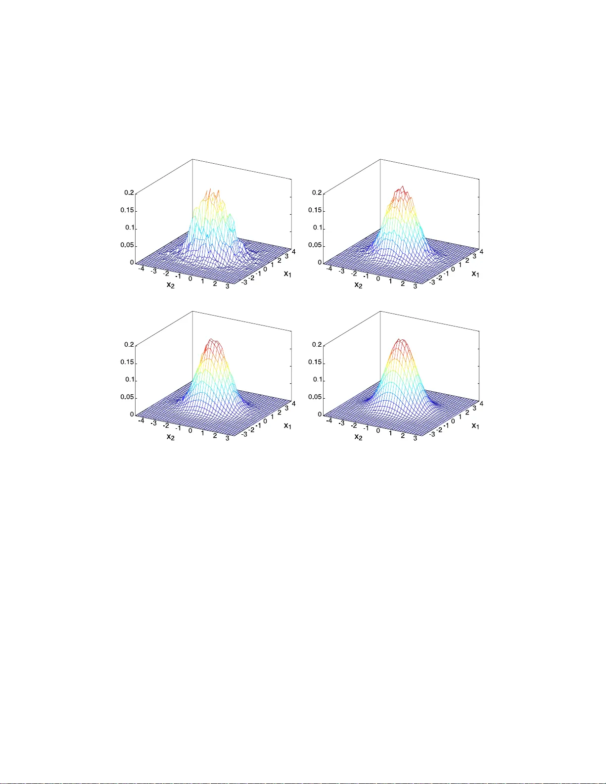
Bernoul li 20 (4), 2014, 1879–19 2 9 DOI: 10.315 0/13-BEJ 545 P article-k ernel estimation of the ﬁlter densit y in state-space mo dels D AN CRISAN 1 and JO AQU ´ ıN M ´ ıGUEZ 2 1 Dep artment of Mathematics , Imp erial Col le ge L ondon, Huxley Building, 180 Que en ’s Gate, L ondon SW7 2BZ, UK. E-mail: d.crisan@imp erial.ac.uk 2 Dep artment of Signal The ory & Comm unic ations, Universidad Carlos III de Madrid, Ave ni da de l a Universidad 30, 28911 L e gan ´ es (Madrid), Sp ain. E-mail: jo aquin.miguez@uc3m.es Sequential Mon t e Carlo (S MC ) metho d s, also kno wn as particle ﬁlters, are sim ulation-based recursive algori t hms for the appro x ima t io n of the a p osterio ri p robab ility measures generated by state-space dynamical mo dels. At any given time t , a SMC metho d prod uces a set of sam- ples ov er the state space o f the system o f in terest (often termed “particles”) t hat is u sed to build a discrete and rand om appro ximation of the posterior p robabili ty d istribution of the state v ariables, conditional on a sequ ence of a va ilable observ ations. One potential app lication of the metho d olo gy is the estimation of the densities associated to the sequence of a p osteriori distri- butions. While practitioners ha ve rather freely applied such density appro ximations in th e past, the issue h as received less attention from a theoretical p erspective. In this paper, we add ress the problem of constructing kernel-based estimates of the p osteri or probabilit y density function and its deriv atives, and obtain asymptotic conv ergence results for th e estimation errors. In par- ticular, we ﬁnd converge n ce rates for t he appro ximation errors that hold un iformly on the state space and guaran tee that the error v anishes almost surely as the num b er of particles in the ﬁlter gro ws. Based on th is unifo rm conv ergence result, w e ﬁrst sho w h ow to build con tinuous measures that con verge almost surely (with known rate) tow ard the p osterior measure and then address a few applications. The latter include maxim um a p os t erio ri estimation of the system state using the app ro ximate deriv atives of the p osterior densit y and the appro x imatio n of functionals of it, for example, Shannon’s entrop y . Keywor ds: density estimation; Marko v systems; particle ﬁltering; sequential Monte Carlo; state-space models; stochastic ﬁltering 1. In tro duction 1.1. Bac kground Consider tw o r a ndom s equences, { X t } t ≥ 0 and { Y t } t ≥ 1 , p ossibly multidimensional, where X t represents the unobser ved state of a sy s tem of interest and Y t is a related observ ation. This is an electronic reprint of th e original article pub lis h ed by the ISI/BS in Bernoul li , 2014, V o l. 20, N o. 4, 1879–1929 . This reprint diﬀers from the original in pagination and typographic detail. 1350-7265 c  2014 ISI/BS 2 D. Crisan and J. M ´ ıguez V er y often, the dep endence betw ee n the tw o seque nc e s is given by a Markov state-space mo del and the p osterior probability mea sure that characterizes the random v ariable X t conditional on the obser v ations { Y s , 1 ≤ s ≤ t } is usually termed the “ﬁltering measure”, denoted as π t in the sequel. If the mo del is linear and Gaussian, π t is also Gaussia n a nd can b e c o mputed exactly using a set of r ecursiv e eq ua tions known a s the K alman ﬁlter [ 32 ]. How ever, if X t takes v alues in a c o n tinuous spa ce a nd the mo del is no nlinear o r non-Gaussian, the exa ct ﬁlter is in trac ta ble and numerical a ppro xima tion techniques are necessary . The cla ss of sequen tia l Monte Carlo (SMC) metho ds, also known as particle ﬁlters [ 21 , 22 , 2 7 , 3 3 , 36 ], has b ecome a very po pular to ol fo r this purpos e. Particle ﬁlters generate discr ete random measures (cons tructed from ra ndom samples in the state spac e ) that can b e naturally used to approximate in tegr als with resp ect to (w.r.t.) the ﬁltering measure. The asymptotic conv erg e nc e of SMC a lgorithms has b een well studied dur ing the past tw o deca des. The ﬁr st formal results app eared in [ 13 , 1 4 ], while the analysis in [ 9 ] already to ok in to acco unt the branching (resampling) step indispe ns able in most practical a pplications. Currently , ther e is a broad knowledge ab out the conv ergence of particle ﬁlters in so me of the forms co mmonly used in practical applications; see [ 3 , 8 , 15 , 16 , 3 0 , 35 ] and the refer ences therein. Most of these res ults are aimed to show that integrals o f r eal functions w.r.t. π t can b e a ccurately approximated by weigh ted sums when the pa r ticle ﬁlter is run with a suﬃciently lar ge num b er of r andom sam- ples (commonly referr ed to as particles). Mor e recently , other types o f conv er gence hav e been inv estigated. F o r instance, the con vergence of particle approximations of maximum a po steriori (MAP) estimates of sequences has also b een proved. Conv er- gence in pr obabilit y ca n b e shown using r andom g e nealogical trees (see [ 40 ] and [ 15 ]) while a lmost sure co n vergence can also be gua r an teed by extending the analy s is in [ 10 ] (see [ 3 8 ]). In most c ases of interest, the ﬁlter ing measure has a density , denoted p t , w.r.t. a domi- nating measure (usually Leb e sgue’s) and practitioners have freely use d v arious estimators of this function. Less attention has been devoted to this pro ble m from a theoretica l p er- sp ectiv e, though. Note that the sa mples generated by the particle ﬁlter ar e not drawn directly from p t : they can only b e co nsidered as appr oximate samples , in the sense that they can b e used to estimate the v alue of integrals w.r.t. the measure π t . As a conse- quence, the convergence of a kernel density estimate of p t built fro m the o utput of a particle ﬁlter c a nnot b e justiﬁed dir ectly using the classica l theory of k er nel density esti- mation, which is concer ned with s amples drawn directly from the dis tr ibution of in tere s t (see, e.g ., [ 18 , 42 , 43 , 45 ]). The estimation of p t is of interest b y itself, since it naturally enables the computation o f conﬁdence regions, a s well as MAP and maximum likelihoo d estimators, but also b ecause it lea ds to the approximation of π t by a contin uous (instea d of discre te) ra ndo m measure. The conv ergence of co n tinuous appr oximations o f the ﬁltering measur e in total v ariation distance has bee n inv estigated in the context of r egularized pa r ticle ﬁlters [ 35 ] as well as for a ccept/reject and auxiliary particle ﬁlter s [ 34 ]. Particle-kernel density estimation 3 1.2. Con tributions In this pap er, we ana ly ze the appr oximation o f p t constructed as the sum of prop erly scaled kernel functions lo cated at the par ticle p ositions. Kernel metho ds [ 42 , 45 ] ar e the most widely used techn iq ues for the no nparametric estimatio n of probability den- sity functions (pdfs) a nd, ther efore, it seems natural to analyze their conv ergence when applied to the approximate samples genera ted by par ticle ﬁlters. The p df estimators we analy z e ar e based on gener ic k ernel functions which are only required to satisfy mild standard conditions (esse n tially the same as in classical densit y es- timation theor y [ 42 ]). W e describ e how to build approximations in ar bitrary-dimensional spaces R d , d ≥ 1 , and then analy z e their co n vergence as the num b er of pa rticles is in- creased a nd the bandwidth of the kernels is decr eased. In par ticular, w e obtain p oint-wise conv erg e nc e rates for the abso lute appr o ximatio n erro rs, b oth of p t and its deriv ativ es 1 (provided they exist). The latter results c an b e extended to deduce uniform (instead of p oin t-wise) conv er g ence rates, a gain bo th for p t and its der iv ativ es. Sp e c iﬁcally , we provide explicit b ounds for the supremum of the a ppro xima tion err or and prove that it conv e r ges almost sure ly (a.s.) tow ar d 0 a s the num b er of particles is incr eased. Our analysis is diﬀerent from the standard metho ds in k er nel density estimation. The la tter address the bias and v ariance of the estimator s using approximations based o n T aylor series (see, e.g., [ 42 ], Chapter 4 or [ 45 ], Chapter 4) or E dgew or th expa nsions [ 2 8 ], which enable the asymptotic approximation o f the mea n integrated square error (MISE) of the density estimate a nd yield ex pressions inv olving the num b er of samples and the kernel bandwidth. W e directly obtain co n vergence r ates for v ar io us estimation err ors (not only the MISE), given in ter ms of a single index that links the num b er of samples and the kernel bandwidth. This link is brieﬂy discussed in Sec tio n 3.3 . The uniform (on the supp ort of p t ) convergence re s ult can b e exploited in a num b er of wa ys. F or instance, if we let p N t be the approximation of p t with N particles, then we can obtain a contin uous appr o ximation o f the ﬁltering measure π t (d x ) as ˘ π N t (d x ) = p N t ( x ) d x , prov e tha t ˘ π N t conv erg e s to π t a.s. in tota l v ariation distance (a s N → ∞ ) and provide explicit conv er gence r ates. A similar kind of a nalysis also lea ds to the calculation of conv erg e nc e rates for the MISE of the particle- kernel density es tima tor p N t . Additionally , we prov e that the (random) in tegr ated square er ror (ISE) of a truncated version of p N t conv erg e s to 0 a.s. and provide conv erg ence rates. A compar ison of these res ults with the standard asymptotic approximation of the MISE for kernel estimators built from i.i.d. samples is prese nted at the end o f Section 4.3 . The conv ergence in total v aria tion distance of a contin uo us approximation of the ﬁlter- ing measure π t was also a ddressed in [ 35 ] and [ 34 ]. Co mpared to these earlier co n tribu- tions, our ana lysis g uarant ee s the almost sure convergence of the (r andom) total v ariation 1 Let us note here that the appro xi m at i on of deriv ativ es of the ﬁlter has receiv ed atten tion recen tly , related to problems of parameter estimation in state-space systems [ 12 , 17 ]. In the latter con text, the ﬁltering pdf is made to depend explicitly on a parameter v ector θ = ( θ 1 , . . . , θ d ), and the in terest is in the computation of the partial deriv ativ es ∂ p t /∂ θ i in order to implement, for example, maximu m li k eliho od estimation algorithms [ 17 ]. In this paper , how ev er, we consider deriv ativ es with resp ect to the state v ariables in X t = ( X 1 ,t , . . . , X d x ,t ), that is, ∂ p t /∂ x i,t . 4 D. Crisan and J. M ´ ıguez distance toward 0, with explicit rates, r ather than the co n vergence of its exp ected v alue (as in [ 35 ]) or its co n vergence in probability (as in [ 3 4 ]). Also, our assumptions on the Marko v kernel of the state pro cess { X t } t ≥ 0 and the conditional densities of { Y t | X t } t ≥ 1 are relatively mild and simple to chec k. In par ticular, our r esults also hold for lig h t-tailed Marko v kernels (e.g., Gaussia n), unlik e Theorems 2 and 3 in [ 34 ]. The last part o f the pap er is devoted to some applications of the density approximation metho d and the uniform conv er gence result. W e ﬁrst consider the problem of MAP estimation. W e refer here to the max imization of the ﬁlter ing dens it y , a problem diﬀeren t from that of MAP estimation in the path s pace addres sed, fo r example, in [ 26 , 38 , 40 ]. W e ﬁrst prov e tha t the maxima of the approximation o f the ﬁltering density a ctually conv erg e , asymptotically , to the maxima of the tr ue function p t and then s ho w some simulation results that illustr a te the use of gr adien t algorithms on the estimated density function. The second application w e descr ibe is the approximation of functionals of p t . W e provide ﬁrs t a gener ic r esult that guarantees the almos t sur e conv erge nce of such ap- proximations for bo unded a nd Lipschitz contin uous functionals. Then, we addr e ss the problem of approximating Shannon entropies [ 7 ], which is of pra c tica l int e r est in v ario us machine le arning and sig nal pro cessing problems. The lo g function is ne ither b ounded nor Lipschitz contin uous and, therefor e, the latter ge ner ic r e sult do es not apply to the computation o f en tr opies. W e sp eciﬁcally a ddress this pro blem resorting to a new r e s ult on the convergence of the particle approximations of int e grals of the fo rm R f ( x ) π t (d x ) when the test function f is p ossibly un b ounded. Let us remark that a large ma jority of the results in the literatur e [ 3 , 8 , 15 , 16 , 35 ] re fer exclus iv ely to the approximation of int eg rals of b ounded functions. Only recently , the conv erge nce of appr o ximate integrals of unbounded test functions has b een prov ed [ 31 ], albeit for a mo diﬁed par ticle ﬁlter and assuming that the pr oduct of the tes t and the likelihoo d functions is bounded. Here , we prove the almost sure con vergence of the a ppro xima tio ns of in teg rals of unbounded functions for the standard particle ﬁlter, pla cing only in tegr abilit y as sumptions o n the test function. F r o m this result, we deduce the almost sure co n vergence tow a r d 0 of the error s in the approximation of Shannon entropies for de ns ities with a co mpact supp ort. A numerical illustra tion is given. 1.3. Organization of the pap er The re s t of the pap er is org anized a s follows. Section 2 co n tains background ma terial, including a summar y of notation, a descr iption of Ma r k ov state s pace models and the standard particle ( b o otstr ap ) ﬁlter. A new lemma that esta blishes the co n vergence of the particle appr o ximatio n of p osterior exp ectations o f un b ounded test functions is a lso in- tro duced in Section 2 . The constr uction of particle-kernel approximations of the ﬁlter ing density and its der iv atives is describ ed in Section 3 , where we a lso r e view some basics of kernel density estimation and the mos t relev an t results in [ 3 5 ] and [ 34 ] for density es ti- mation with particle ﬁlters. O ur formal re s ults on the conv erge nce of the pa rticle-k er nel density estimato r s and the s mooth appr o ximation of the ﬁlter ing measure are introduced Particle-kernel density estimation 5 in Section 4 . This includes the p oin t-wis e and unifor m approximations of p t ( x ), the co n- vergence in total v ariation dis tance of the smo oth mea sures ˘ π N t and conv ergence rates for the mean in teg rated squar e erro r and the (random) integrated squar e e r ror of p N t and its truncated version, res pectively . In Section 5 , we discuss applications of the particle-kernel estimator of p t and its deriv atives. In particular , we consider the problem of (marginal) MAP estimation of the s tate v ar iables and the appr o ximatio n of functiona ls of the ﬁl- tering density , including Sha nnon’s entrop y . Finally , brief conclusions ar e presented in Section 6 . 2. P article ﬁltering 2.1. Notation W e ﬁrst int r oduce some common no ta tions to b e used through the pap er, broadly clas s i- ﬁed by topics. Below, R denotes the real line, while for an in teger d ≥ 1 , R d = d times z }| { R × · · · × R • Measures a nd in teg rals. – B ( R d ) is the σ -algebra of Borel s ubsets of R d . – P ( R d ) is the set of proba bilit y measure s o ver B ( R d ). – ( f , µ ) , R f ( x ) µ (d x ) is the integral of a real function f : R d → R w.r.t. a measure µ ∈ P ( R d ). – T ake a measure µ ∈ P ( R d ), a Borel set A ∈ B ( R d ) and a real function f : R d → R + . The pr o jective pro duct f ⋆ µ is a measure, absolutely contin uous w.r.t. µ a nd prop ortional to f , constructed as ( f ⋆ µ )( A ) = R A f ( x ) µ (d x ) ( f , µ ) . (2.1) • F unctio ns . – The supremum norm of a real function f : R d → R is denoted as k f k ∞ = sup x ∈ R d | f ( x ) | . – B ( R d ) is the set of bo unded real functions ov er R d , that is, f ∈ B ( R d ) if, and only if, k f k ∞ < ∞ . – C b ( R d ) is the set of contin uous and b ounded real functions over R d . • Sets. – Given a probability mea sure µ ∈ P ( R d ), a Bo r el set A ∈ B ( R d ) and the indica tor function I A ( x ) =  1 , if x ∈ A, 0 , otherwise , µ ( A ) = ( I A , µ ) = R A µ (d x ) is the probability of A . – The Leb esgue mea sure of a set A ∈ B ( R d ) is denoted L ( A ). – F o r a set A ∈ R d , A c = R d \ A denotes its complement. 6 D. Crisan and J. M ´ ıguez • Sequences, vectors a nd random v a riables (r.v.). – W e use a subscript notation fo r sequences, x t 1 : t 2 , { x t 1 , . . . , x t 2 } . – F o r a n element x = ( x 1 , . . . , x d ) ∈ R d of an Euclidean space, its nor m is deno ted as k x k = p x 2 1 + · · · + x 2 d . – The L p norm of a real r.v. Z , with p ≥ 1 , is written as k Z k p , E [ | Z | p ] 1 /p , where E [ · ] denotes exp ectation. 2.2. Filtering in discrete-time, state-space Mark o v mo dels Consider tw o rando m sequences, { X t } t ≥ 0 and { Y t } t ≥ 1 , taking v alues in R d x and R d y , resp ectiv ely . The common proba bilit y measur e for the pair ( { X t } t ≥ 0 , { Y t } t ≥ 1 ) is denoted P , and we assume that it is absolutely contin uous w.r.t. the Leb esgue measur e. W e refer to the ﬁrst sequence as the state pr ocess and we a ssume that it is an inhomog e ne o us Marko v chain governed b y an initial pro babilit y measure τ 0 ∈ P ( R d x ) and a s equence of transition kernels τ t : B ( R d x ) × R d x → [0 , 1] , deﬁned as τ t ( A | x t − 1 ) , P { X t ∈ A | X t − 1 = x t − 1 } , (2.2) where A ∈ B ( R d x ) is a Borel set. The sequence { Y t } t ≥ 1 is termed the observ ation pro cess. Each r.v. Y t is assumed to b e co nditionally indep endent of other obser v ations given the state X t , meaning that P { Y t ∈ A | X 0: t = x 0: t , { Y k = y k } k 6 = t } = P { Y t ∈ A | X t = x t } (2.3) for any A ∈ B ( R d y ). Additionally , we as sume that every probability mea sure γ t ∈ P ( R d y ) in the seq uence γ t ( A | x t ) , P { Y t ∈ A | X t = x t } , A ∈ B ( R d x ) , t = 1 , 2 , . . . , (2.4) has a p ositiv e density w.r.t. the Leb esgue measure . W e denote this dens ity as g t ( y | x ), hence we wr ite γ t ( A | x t ) = R A g t ( y | x t ) d y . The ﬁltering problem consists in the computation o f the pos terior pr obabilit y measure of the state X t given a se q uence of obse rv ations up to time t . Sp eciﬁcally , for a ﬁxed observ ation r ecord Y 1: T = y 1: T , T < ∞ , we seek the measures π t ∈ P ( R d x ) given b y π t ( A ) , P { X t ∈ A | Y 1: t = y 1: t } , t = 0 , 1 , . . . , T , (2.5) where A ∈ B ( R d x ). F o r many practical proble ms , the interest actually lies in the compu- tation of integrals of the for m ( f , π t ). No te that, for t = 0, we recov er the pr ior mea sure, that is, π 0 = τ 0 . Particle-kernel density estimation 7 2.3. P article ﬁlters The seq ue nc e of mea sures { π t } t ≥ 1 can b e n umeric a lly approximated using par ticle ﬁlter- ing. Particle ﬁlters a re n umeric a l metho ds based on the re c ursiv e dec omposition [ 3 ] π t = g y t t ⋆ τ t π t − 1 , (2.6) where g y t t : R d x → R + is the function deﬁned as g y t t ( x ) , g t ( y t | x ), ⋆ denotes the pro jective pro duct and ξ t , τ t π t − 1 is the (predictive) pr o babilit y meas ure ξ t ( A ) = τ t π t − 1 ( A ) = Z τ t ( A | x ) π t − 1 (d x ) , A ∈ B ( R d x ) . (2.7) Spec iﬁc a lly , the simplest pa rticle ﬁlter, often called ‘s tandard particle ﬁlter’ or ‘b o otstrap ﬁlter’ [ 27 ] (see also [ 20 ]), can b e descr ib ed as follows. 1. Initialization. At time t = 0 , draw N i.i.d. samples fr o m the initia l distribution τ 0 ≡ π 0 , denoted x ( n ) 0 , n = 1 , . . . , N . 2. R e cursive step. Let Ω N t − 1 = { x ( n ) t − 1 } n =1 ,...,N be the par ticles (samples) generated at time t − 1. A t time t , pro ceed with the t wo steps b elo w. (a) F or n = 1 , . . . , N , draw a sample ¯ x ( n ) t from the pr obabilit y distr ibution τ t ( ·| x ( n ) t − 1 ) and compute the nor ma lized weigh t w ( n ) t = g y t t ( ¯ x ( n ) t ) P N k =1 g y t t ( ¯ x ( k ) t ) . (2.8) (b) F o r n = 1 , . . . , N , let x ( n ) t = ¯ x ( k ) t with pr obabilit y w ( k ) t , k ∈ { 1 , . . . , N } . Step 2 (b) is referr ed to as resampling or selectio n. In the form sta ted her e, it reduces to the so-called m ultinomia l r esampling algo rithm [ 19 , 22 ] but the co nvergence of the algorithm ca n be ea sily prov ed for v arious other schemes (see, e.g., the trea tmen t of the resampling step in [ 8 ]). Using the samples in Ω N t = { x ( n ) t } n =1 ,...,N , we construct a r andom approximation of π t , namely π N t (d x t ) = 1 N N X n =1 δ x ( n ) t (d x t ) , (2.9) where δ x ( n ) t is the delta unit-measure lo cated at X t = x ( n ) t . F or any integrable function f in the sta te space, it is straightforward to approximate the in teg ral ( f , π t ) as ( f , π t ) ≈ ( f , π N t ) = 1 N N X n =1 f ( x ( n ) t ) . (2.10) 8 D. Crisan and J. M ´ ıguez The convergence of particle ﬁlters has b e en analyz e d in a num b er o f diﬀeren t wa ys . Most o f the results to b e describ ed in this pap er rely only o n the conv erg ence of the L p norm of the appr oximation er rors ( f , π N t ) − ( f , π t ) for b ounded functions. Additionally , we establis h the a .s. conv erg e nc e tow ar d 0 of the a ppr o ximatio n er rors for a clas s o f po ssibly un b ounded functions. Speciﬁca lly , let f b e a real function over the sta te space and intro duce the notation τ t ( f )( x ) = Z f ( z ) τ t (d z | x ) for c onciseness. Note that τ t ( f ) : R d x → R is als o a real function ov er the state space. W e deﬁne the following class of functions. Deﬁnition 2.1. F p T is a family of fu n ctions f : R d x → R that satisfy: (i) ( f p , π t ) < ∞ for t = 0 , . . . , T , and (ii) if f ∈ F p T then τ t ( f p ) ∈ F p T for t = 1 , . . . , T . The set F p T includes functions tha t a re p - in tegrable w.r.t. π t , 0 ≤ t ≤ T , and remain p -integrable when sequentially transformed by the kernels τ t , 1 ≤ t ≤ T . Note that if p ≤ q then F q T ⊆ F p T . It turns o ut that if f ∈ F p T for some p ≥ 4, then the error o f the particle approximations v anishes fo r large N at every time step. This is precisely s tated by the following prop osition. Prop osition 2.1. Ass ume that the se qu enc e of observations Y 1: T = y 1: T is ﬁ xe d, with T b eing some lar ge but ﬁnite time horizon, g y t t ∈ B ( R d x ) and g y t t > 0 (in p articular, ( g y t t , ξ t ) > 0 ) for every t = 1 , 2 , . . . , T . The fol lowi ng r esults hold. (a) F or any f ∈ B ( R d x ) and any p ≥ 1 , k ( f , π N t ) − ( f , π t ) k p ≤ c t k f k ∞ √ N (2.11) for t = 0 , 1 , . . . , T , wher e c t is a c onstant indep endent of N , k f k ∞ = sup x ∈ R d x | f ( x ) | and t he exp e ctation is taken over al l p ossible r e alizations of the ra n dom me asur e π N t . In p articular, lim N →∞ | ( f , π N t ) − ( f , π t ) | = 0 a.s. for 0 ≤ t ≤ T . (b) If f ∈ F 4 T , then lim N →∞ | ( f , π N t ) − ( f , π t ) | = 0 a.s. for 0 ≤ t ≤ T . See App endix A fo r a pr oof. R emark 2.1. Part (a) of Pr opositio n 2.1 is fairly standard. A similar prop osition was already pr o ved in [ 1 6 ], alb eit under additiona l a ssumptions on the state-spac e mo del. Bounds for p = 2 and p = 4 ca n also b e found in a n umber of references (see, e.g., Particle-kernel density estimation 9 [ 8 , 11 , 15 ]). Part (b) es ta blishes the a lmost sure conv erge nce for the approximate in- tegrals o f unbounded functions (e.g., for the appr o ximatio n of the p osterior mean) as long as they are “suﬃciently integrable”. A similar result can b e found in [ 31 ], including conv erg e nc e rates. How ever, the analysis in [ 31 ] is car ried out for a mo diﬁed particle ﬁltering algor ithm, that involv es a rejection test on the generated par ticles, and cannot be a pplied to the standard par ticle ﬁlter presented in this se ction. 3. P article-k ernel app r o ximation of the ﬁltering densit y In the s equel, we will b e concer ned with the family of Ma rk ov sta te-space mo dels for which the p osterior probability measure s { π t } t ≥ 1 are abso lutely contin uous w.r.t. the Leb esgue measure and, therefore , there exis t pdfs p t : R d x → [0 , + ∞ ), t = 1 , 2 , . . . , such that π t ( A ) = R A p t ( x ) d x fo r any A ∈ B ( R d x ). The densit y p t is r eferred to as the ﬁltering pdf at time t . In this section, we brieﬂy r eview the basic metho dology for kernel densit y estimation and then describ e the construction of s equences of appr o ximations of p t using the particles genera ted by a particle ﬁlter a nd a generic kernel function. The sec tion concludes with the discussion on the relationship betw een the complexity of the particle ﬁlter (i.e., the num b er of particles N ) and the choice o f kernel bandwidth for the density estimators. 3.1. Kernel density estimators In o r der to build an approximation o f the function p t ( x ) using a s a mple of size N , { x ( n ) t } i =1 ,...,N , we reso rt to the class ical kernel appro a c h commonly used in density esti- mation [ 42 , 43 , 4 5 ]. Sp eciﬁcally , given a kernel function φ : R d x → R + , w e build a regu- larized density function of the form p N t ( x ) = 1 N N X n =1 φ ( x − x ( n ) t ) . (3.1) In the clas sical theory , the kernel function φ is often taken to b e a nonnegative and symmetric proba bilit y density function with zero mean and ﬁnite second order mo ment. Spec iﬁc a lly , the following assumptions are commonly made [ 4 2 ] a nd we abide by them in this pap er. A. 1. The kernel φ is a p df w.r.t. the L eb esgue me asur e. In p articular, φ ( x ) ≥ 0 ∀ x ∈ R d x and R φ ( x ) d x = 1 . A. 2. The pr ob ability distribution with density φ has a ﬁnite se c ond or der moment, that is, c 2 = R k x k 2 φ ( x ) d x < ∞ . 10 D. Crisan and J. M ´ ıguez Given a function φ satisfying A. 1 and A. 2 it is p ossible to deﬁne a family of rescaled kernels φ 1 /h ( x ) = h − d x φ ( h − 1 x ) , (3.2) where h > 0 is often referred to as the bandwidth of the kernel function. Both the ker- nel a nd the bandwidth can be optimized to minimize the mean integrated sq ua re error (MISE) b et ween the r egularized density and the targ et densities [ 45 ]. Sp eciﬁcally , the MISE is deﬁned as MISE ≡ Z E " p t ( x ) − 1 N N X n =1 φ 1 /h ( x − x ( n ) t ) ! 2 # d x, (3.3) where the ex pectation is taken ov er the r andom sa mple. Although the MISE g iv en in equation ( 3.3 ) is in tr actable in genera l, as ymptotic appr o ximations (as N → ∞ ) are known [ 45 ]. Moreov er , if we ass ume that x (1) t , . . . , x ( N ) t are i.i.d. and drawn exactly from p t ( x ) (b ew a re that this is not the case in the particle ﬁlter ing framework, thoug h), then the MISE is minimized by the E panec hnikov kernel [ 42 ] φ E ( x ) =    d x + 2 2 v d x (1 − k x k 2 ) , if k x k < 1 , 0 , otherwise , (3.4) where v d x is the volume of the unit sphere in R d x . If, additionally , p t ( x ) is Gaussia n with unit cov aria nce ma trix, then the s caling of φ E that yields the minimu m MISE is given by the bandwidth [ 45 ] h opt = [8 v − 1 d x ( d x + 4)(2 √ π ) d x ] 1 / ( d x +4) N − 1 / ( d x +4) . In our ca s e, p t ( x ) is not known (it is known not to b e Gauss ian in genera l, though) and the rando m sample x (1) t , . . . , x ( N ) t is not drawn from p t ( x ), so the standard res ults of [ 42 , 43 , 45 ] and others canno t b e applied dire c tly and a s peciﬁc a nalysis is needed [ 34 , 35 ]. In [ 35 ], tw o r egularized par ticle ﬁltering algorithms were studied, each of them yielding a diﬀer en t kernel estima tor of p t . Using the notation in the present paper , they can b e written as p N t, pre ( x ) ∝ 1 N N X n =1 g t ( y t | x ) φ 1 /h ( x − ¯ x ( n ) t ) (3.5) for the pr e-r e gularize d p article ﬁlter , and p N t, p ost ( x ) = N X n =1 w ( n ) t φ 1 /h ( x − ¯ x ( n ) t ) Particle-kernel density estimation 11 for the p ost-regula rized par ticle ﬁlter. Note that p N t, pre ( x ) is an unnor malized approx- imation o f p t ( x ) (the norma lization c o nstan t cannot be computed in ge neral). F or the po st-regularized density estimator, it can b e shown that under ce r tain regular ity assump- tions ([ 35 ], Theorem 6 .15) E  Z | p t ( x ) − p N t, p ost ( x ) | d x | Y 1: t  → 0 a.s. (where the ex pectation is taken w.r.t. p N t, p ost ) when N → ∞ and h → 0 join tly . Sp eciﬁcally , the mean total v a riation decrea ses as O( N − 1 / 2 + h 2 ). A similar re s ult can be sho wn for p N t, p ost ([ 35 ], Theorem 6 .9). R emark 3.1. Although we use the same notation for the par ticles, ¯ x ( i ) t , i = 1 , . . . , N , as in Sectio n 2.3 , the s ampling/resampling schemes in the pre-reg ula rized and p ost- regular iz ed par ticle ﬁlter s are diﬀerent from the basic ‘b o otstra p’ ﬁlter [ 35 , 39 ]. The pre-reg ula rized ﬁlter , in pa rticular, inv olves the use o f a re jectio n sampler. R emark 3.2. The conv erg ence r esults in [ 35 ] for the po st-regularized densit y estimato r p N t, p ost hold true when the following as sumptions on the state-space mo del are guaranteed. • The transition kernel R t ( x t − 1 , A ) = R A g Y t t ( x ) τ t (d x | x t − 1 ) is mixing ([ 35 ], Deﬁni- tion 3.2 ). • The likelihoo d satisﬁes sup u ∈ W 2 , 1 g Y t t u k u k 2 , 1 < ∞ , where W 2 , 1 is the So bolev spac e of functions deﬁned on R d x which, together with their der iv atives up to order 2, are int eg rable with resp ect to the Leb esgue measur e , a nd k · k 2 , 1 is the corr esponding norm. • The meas ure τ t (d x | x t − 1 ) is absolutely con tinuous w.r.t. the Leb esgue measur e, with density τ x t − 1 t ( x ) ∈ W 2 , 1 and sup x t − 1 ∈ R d x k τ x t − 1 t k 2 , 1 < ∞ . Assuming that τ t = τ for every t ≥ 1 (hence, the Marko v state pro cess is homogeneo us), the analysis in [ 34 ] targets the conv erg ence in total v aria tion distance of the contin uous measure ρ N t ( x ) d x , where the density estimato r ρ N t is deﬁned as ρ N t ( x ) = c t N X n =1 g t ( y t | x ) τ x ( n ) t − 1 ( x ) with normalization constant c t = ( P N n =1 R g t ( y t | x ) τ x ( n ) t − 1 ( x ) d x ) − 1 . This is simila r to the pre-reg ula rized approximation p N t, pre but using the Marko v kernel of the mo del, τ , fo r smo othing, instead of the generic kernel φ 1 /h . Although in most pro blems it is p ossible to draw fr o m τ x t − 1 , it is o ften not po ssible to ev aluate it a nd, in such cases, the approx- imation ρ N t is not pr actical. Also no te that ρ N t is not a kernel density estimator of p t in the classical form of equation ( 3.1 ). The sample of size N fro m which the approxima- tion is co nstructed corresp onds to the v ar iable X t − 1 , r a ther than X t , and smoo thing is 12 D. Crisan and J. M ´ ıguez achiev ed by wa y o f a prediction step (using the Ma rk ov kernel τ ). It is not p ossible, in general, to wr ite ρ N t ( x ) ∝ P N n =1 g t ( y t | x ) φ 1 /h ( x − x ( n ) t − 1 ) for some kernel function φ . Under regular ity assumptions o n g t and τ , it is prov ed in [ 34 ], Theor em 2, that P  Z | ρ N t ( x ) − p t ( x ) | d x > ǫ  ≤ c 1 exp {− c 2 N } , t ≥ 1 , (3.6) for a n y ǫ > 0 and so me constants c 1 , c 2 > 0 . R emark 3.3. The regularity a ssumptions o n the state-space mo del in [ 34 ], Theor em 2, are the following. (a) There ar e p dfs { b t } t ≥ 1 and t wo co nstan ts 0 < c τ < C τ < ∞ such that c τ b t ( x ) ≤ τ x t − 1 ( x ) ≤ C τ b t ( x ) for a ll x, t. (b) The lik e liho o d g t satisﬁes that s up t ≥ 1; x,x ′ ∈ R d x ; y ∈ R d y g t ( y | x ) g t ( y | x ′ ) < ∞ . The a ssumption in (a) excludes, for exa mple, mo dels of the for m X t = h ( X t − 1 ) + V t where the function h : R d x → R d x is not b o unded or the noise pr ocess V t is Gaussian ([ 34 ], Section 4.2). The as sumption in (b) is also str onger than requir e d for Prop osition 2.1 to hold true. 3.2. Appro ximation of t he ﬁltering densit y and its deriv ativ es W e inv estig ate particle-kernel approximations o f p t constructed from a kernel function φ and the s a mples x ( n ) t , n = 1 , . . . , N , genera ted b y the particle ﬁlter. Instead of r estricting our attention to pro cedures based on a sing le k er nel, how ever, we consider a s e quence of functions φ k : R d x → R + , k ∈ N , deﬁned according to the notation in equation ( 3.2 ), that is, φ k ( x ) = k d x φ ( k x ). If φ complies with A. 1 a nd A. 2 , then we hav e similar prop erties for φ k . T rivially , φ k ( x ) ≥ 0 ∀ x ∈ R d x , and it is als o str a igh tforward to c heck that R φ k ( x ) d x = 1. Moreover, if we apply the change of v ariable y = k x and note that d y = k d x d x , then Z k x k 2 φ k ( x ) d x = 1 k 2 Z k y k 2 φ ( y ) d y = c 2 k 2 from A. 2 . The appr oximation of p t generated by the pa rticles x ( n ) t , n = 1 , . . . , N , a nd the k th kernel, φ k , is denoted as p k t and has the form p k t ( x ) , 1 N N X n =1 φ k ( x − x ( n ) t ) = ( φ x k , π N t ) , where φ x k ( x ′ ) , φ k ( x − x ′ ). Beware that, in o ur notation, we skip the dep endence of p k t on the num b e r of particles, N , for the sa k e of simplicity . In Se c tio n 4.1 , we will assume Particle-kernel density estimation 13 a c ertain r elationship b et ween N and k that will be car ried on through the rest of the pap er and justiﬁes the omissio n in the notation. Let us also remark that we do not construct p k t in order to approximate in teg rals w .r .t. the ﬁltering measure (this is more eﬃciently achiev ed using equation ( 2.10 )). Instead, we aim at applica tions where an explicit approximation of the density p t is necessar y . Some examples ar e co ns idered in Section 5 . In order to inv estiga te the approximation o f deriv atives of p t , let us conside r the m ulti- index α = ( α 1 , α 2 , . . . , α d x ) ∈ N ∗ × N ∗ × · · · × N ∗ , where N ∗ = N ∪ { 0 } , and in tro duce the partial der iv ative op erator D α deﬁned as D α h , ∂ α 1 · · · ∂ α d x h ∂ x α 1 1 · · · ∂ x α d x d x for a n y (suﬃcien tly diﬀerentiable) function h : R d x → R . The order of the deriv ative D α h is denoted a s | α | = P d x i =1 α i . W e ar e interested in the approximation of functions D α p t ( x ) which are co n tinuous, as explicitly given b elow. A. 3. F or every x in the domain of p t ( x ) , D α p t ( x ) exists and is Lipschitz c ontinuou s , that is, ther e exists a c onstant c α,t > 0 such that | D α p t ( x − z ) − D α p t ( x ) | ≤ c α,t k z k for al l x, z ∈ R d x . R emark 3.4. It is p ossible to chec k whether A. 3 holds by insp ecting the transitio n kernel τ t and the likeliho od function g y t t . F o r example, assume that τ t (d x | x ′ ) has a n asso ciated densit y w.r.t. the Leb esgue meas ure, denoted τ x ′ t . A suﬃcient condition for D α p t to b e Lipschitz is tha t both g y t t and τ x ′ t be b ounded with b ounded der iv atives up to order 1 + | α | . Sp eciﬁcally , it is s uﬃcien t that g y t t ∈ B ( R d x ) and, for a ny β = ( β 1 , . . . , β d x ) such that 0 ≤ | β | ≤ 1 + | α | , D β g y t t ∈ B ( R d x ) and there exis t consta n ts c β , indep enden t of x and x ′ , such that D β τ x ′ t ≤ c β . F o r the same α , we also imp ose the following condition o n the k er nel φ . A. 4. D α φ ∈ C b ( R d x ) , that is, D α φ is a c ontinuous and b oun de d funct ion. In p articular, k D α φ k ∞ = sup x ∈ R d x | D α φ ( x ) | < ∞ . R emark 3.5. T rivia lly , if D α φ ∈ C b ( R d x ) then D α φ k ∈ C b ( R d x ) for any ﬁnite k . In particular, k D α φ k k ∞ = k d x + | α | k D α φ k ∞ . The appr o ximation of D α p t computed fro m the sa mples x ( n ) t , n = 1 , . . . , N , and the k th kernel, φ k , has the form D α p k t ( x ) = 1 N N X n =1 D α φ x k ( x ( n ) t ) = ( D α φ x k , π N t ) . (3.7) 14 D. Crisan and J. M ´ ıguez 3.3. Complexit y of t he particle ﬁlter and c hoice of kernel bandwidth In the seque l, we will b e concerned with the conv erg ence of the sequence of approx- imations { D α p k t } k ≥ 1 under the gener ic ass umptions A. 1 –A. 4 . The convergence results int r oduced in Sections 4 and 5 are given either as limits, for k → ∞ , or as erro r b ounds that decrease with k . Recall, how ever, that p k t ( x ) = ( φ x k , π N t ), that is, the density estimator p k t depe nds b oth on the kernel bandwidth h = 1 k and the nu mber of particles N . A distinctive feature o f the ana ly sis in Sections 4 a nd 5 is that it links b oth indices by way o f the ineq ua lit y N ≥ k 2( d x + | α | +1) , where | α | = P d x i =1 α i is the order of the der iv ative D α . F o r α = (0 , . . . , 0), D α p k t = p k t and N ≥ k 2( d x +1) . (3.8) Obviously , k → ∞ implies that N → ∞ and h → 0. This co nnection is useful to provide simple bounds for the approximation error s , but also b ecause it y ields guidance for the n umeric al implemen tation of the density estima- tors. In particular, for | α | = 0 a nd a ﬁxed k er nel ba ndwidth h = 1 k , the inequality in ( 3.8 ) determines the minimum n umber o f particles N that ar e needed in the particle ﬁlter in order to guara n tee that conv ergence, at the rates given b y the Theorems of Sections 4 and 5 , holds. A les s er num b er of samples (i.e., s ome N < k 2( d x +1) ) would result in an under-smo othed density p k t ( x ) with a big ger approximation error . If the computational complexity of the particle ﬁlter is limited b y practical con- siderations, then N is given and the erro r b ounds to be introduced o nly hold when k ≤ N 1 / (2( d x +1)) or, equiv alently , when the kernel bandwidth is low er- b ounded as h = 1 k ≥ N − 1 / (2( d x +1)) . A smaller bandwidth would, again, result in an under-smo othed approxi- mation p k t ( x ). On the other hand, since ov er-smo othing also increa ses the a ppro xima tion error of kernel dens it y estimator s [ 42 ], it is conv enient to choose the smallest p ossible bandwidth h . F or given N , we should therefore sele ct 2 h = h ( N ) = N − 1 / (2( d x +1)) . 4. Con v ergence of the appr o x imations Starting from Prop osition 2.1 , we prove that the k er nel appr o ximations of the ﬁltering pdf, p k t ( x ), and its deriv ates conv erg e a .s. for ev er y x in the do ma in of p t , b oth point- wise and uniformly o n R d x . W e also prov e that the s moothed approximating measure ˘ π N ( k ) t (d x ) = p k t ( x ) d x conv erg es to π t in total v aria tion distance and that the integrated square e r ror o f a sequence of tr uncated density e s timators conv erg es q uadratically (in k ) tow ard 0 a.s. Explicit c o n vergence rates for the approximations a re given. 2 In practice, an adaptiv e c hoice of the kernel bandwidth (see, e.g., [ 5 , 47 ]) i s generally more eﬃcient. In this pap er, how ev er , we restrict our attent ion to ﬁxed-bandwidth kernels. Particle-kernel density estimation 15 4.1. Almost sure con vergence In this section, w e obtain con vergence rates f o r the particle - k ernel approximation D α p k t ( x ) of eq uation ( 3.7 ). Dep ending on the supp ort of the density p t ( x ), these rates may b e p oint-wise or uniform (for all x ). In b oth ca ses, conv erg ence is attained a .s. based on the following aux ilia ry result. Lemma 4 .1. L et { θ k } k ∈ N b e a se quenc e of nonne gative r andom variables su ch that, for p ≥ 2 , E [( θ k ) p ] ≤ c k p − ν , ( 4 .1) wher e c > 0 and 0 ≤ ν < 1 ar e c onstant w.r.t. k . Then, ther e exists a nonne gative and a.s. ﬁn it e r andom variable U ε , indep endent of k , such that θ k ≤ U ε k 1 − ε , (4.2) wher e 1+ ν p < ε < 1 is also a c onst ant w.r.t. k . Pro of. See App endix B .  R emark 4. 1. In Lemma 4.1 , if the inequa lity ( 4.1 ) holds for all p ≥ 2 then the constant ε in ( 4.2 ) c an be made a rbitrarily small, that is, we can choose 0 < ε < 1. Using Lemma 4.1 , it is p ossible to prove that D α p k t ( x ) → D α p t ( x ) a.s. and obtain explicit convergence rates. In order to establish a connection b et ween the sequence of kernels φ k ( x ), k ∈ N , and the s e q uence of measure appr oximations π N t , N ∈ N , we deﬁne the num b er of particles to b e a function of the kernel index and denote it as N ( k ). T o b e sp eciﬁc, fo r a given m ulti- index α , w e assume that N ( k ) ≥ k 2( d x + | α | +1) . In this wa y , all the con vergence ra tes to be prese n ted in this pap er are primar ily given in terms of the kernel index k . W e ﬁrst show that D α p k t → D α p t po in t-wise for x ∈ R d x . Theorem 4. 1. Under assumptions A . 1 , A. 2 , A. 3 , A . 4 and N ( k ) ≥ k 2( d x + | α | +1) , the ine quality | D α p k t ( x ) − D α p t ( x ) | ≤ V x,α,ε k 1 − ε (4.3) holds true, with V x,α,ε an a.s. ﬁnite, nonne gative r andom variable and a c onstant 0 < ε < 1 . In p articular, lim k →∞ | D α p k t ( x ) − D α p t ( x ) | = 0 a.s. (4.4) Pro of. Let us construct an appr o ximation o f p t ( x ) using the kernel φ k and the true ﬁltering mea sure π t , namely , ˜ p k t ( x ) = ( φ x k , π t ). Since π t (d x ) = p t ( x ) d x , the approximation 16 D. Crisan and J. M ´ ıguez ˜ p k t is actually a conv o lution integral a nd can b e written in tw o alter na tiv e wa ys using the commutativ e prop ert y , namely ˜ p k t ( x ) = Z φ k ( x − z ) p t ( z ) d z = Z φ k ( z ) p t ( x − z ) d z . (4.5) Let us now consider the deriv ative D α p t . If w e apply the op e rator D α to ˜ p k t in ( 4.5 ), we readily o bta in D α ˜ p k t ( x ) = Z φ k ( z ) D α p t ( x − z ) d z and, us ing the latter expression, w e ﬁnd an upper b ound for the erro r | D α ˜ p t k ( x ) − D α p t ( x ) | . In pa rticular, | D α ˜ p t k ( x ) − D α p t ( x ) | =     Z φ k ( z ) D α p t ( x − z ) d z − D α p t ( x )     ≤ Z φ k ( z ) | D α p t ( x − z ) − D α p t ( x ) | d z (4.6) ≤ c α,t Z φ k ( z ) k z k d z (4.7) ≤ c α,t s Z φ k ( z ) k z k 2 d z (4.8) = c α,t √ c 2 k , (4.9) where equation ( 4.6 ) follows from A. 1 (namely , φ ≥ 0), ( 4.7 ) is obtained from the Lipsc hitz assumption A. 3 , ( 4.8 ) follows from Jensen’s inequality a nd, ﬁnally , the b ound in ( 4.9 ) is obtained from a ssumption A. 2 . Note that c α,t and c 2 are constants with resp ect to b oth x and k . As a consequence of ( 4.9 ), lim k →∞ D α ˜ p k t ( x ) = D α p t ( x ) . Consider now the approximation, with N ( k ) particles, D α p k t = ( D α φ x k , π N ( k ) t ) of the int eg ral ( D α φ x k , π t ). F rom Prop osition 2.1 and ass umption A. 4 , w e obtain k D α p k t ( x ) − D α ˜ p k t ( x ) k p = k ( D α φ x k , π N ( k ) t ) − ( D α φ x k , π t ) k p (4.10) ≤ ¯ c t k d x + | α | k D α φ k ∞ p N ( k ) , where we have used Remar k 3.5 and the constant ¯ c t is independent o f N ( k ) and x . A s traigh tfor w ard application of the tria ngle inequality now yields k D α p k t ( x ) − D α p t ( x ) k p ≤ k D α p k t ( x ) − D α ˜ p k t ( x ) k p + k D α ˜ p k t ( x ) − D α p t ( x ) k p . (4.11) Particle-kernel density estimation 17 The ﬁrst term on the r igh t-hand side of ( 4.11 ) can b e bo unded using ( 4 .10 ), while the second term also has an upp er bo und given by 3 ( 4.9 ). T aking bo th b ounds together, we arrive at k D α p k t ( x ) − D α p t ( x ) k p ≤ ¯ c t k d x + | α | k D α φ k ∞ p N ( k ) + c α,t √ c 2 k ≤ ¯ c α,t k , (4.12) where the second inequality follows from the ass umption N ( k ) ≥ k 2( d x + | α | +1) and ¯ c α,t = ¯ c t k D α φ k ∞ + c α,t √ c 2 ,α is a constant. The inequa lity ( 4.12 ) immediately yields E [ | D α p k t ( x ) − D α p t ( x ) | p ] ≤ ¯ c p α,t k p (4.13) and w e can a pply Lemma 4.1 , with θ k = | D α p k t ( x ) − D α p t ( x ) | , ν = 0 a nd arbitrar ily large p ≥ 2 , to obtain | D α p k t ( x ) − D α p t ( x ) | ≤ V α,x,ε k 1 − ε , (4.14) where V α,x,ε is a nonnegative a nd a.s. ﬁnite random v aria ble a nd 0 < ε < 1 is a constant, bo th of them independent of k . The limit in equation ( 4.4 ) follows immediately from the inequality ( 4.14 ).  R emark 4. 2. The conv erg ence rate for the appr o ximation error k D α p k t ( x ) − D α p t ( x ) k p given by inequality ( 4.12 ) can b e improv ed if we place additional ass umptions o n the ﬁlter density and the kernel, and incr ease the num b er of particles N ( k ). In particular, if in addition to A. 1 –A. 4 w e as sume that • p t ( x ) has co n tinuous and b ounded deriv atives up to or de r | α | + 2 , • the kernel satis ﬁe s R z i φ ( z ) d z = 0, for i = 1 , . . . , d x , and • N ( k ) ≥ k 2( d x + | α | +2) , then it can b e shown, using the m ultiv aria te version of T a y lo r’s theo rem, that k D α p k t ( x ) − D α p t ( x ) k p ≤ ¯ C α,t k 2 for some constant ¯ C α,t independent of k . A spe c iﬁc result that relies o n these extended assumptions is given in Theore m 4.6 (see Section 4.3 ). R emark 4.3. The constant ¯ c α,t of equa tion ( 4.12 ) is indep endent of the index k a nd the po in t x ∈ R d x . The r andom v ar ia ble V α,x,ε is also indep enden t of the kernel index k , as explicitly given by Lemma 4.1 . How ever, it may dep end on the multi-index α , the 3 Note that k D α ˜ p k t ( x ) − D α p t ( x ) k p = | D α ˜ p k t ( x ) − D α p t ( x ) | because D α ˜ p t k ( x ) does not dep end on π N ( k ) t . 18 D. Crisan and J. M ´ ıguez dimension of the state space d x and the p oint x where the deriv ative of the dens it y is approximated, hence the notation. R emark 4. 4. F o r α = (0 , . . . , 0) = 0 , the inequality ( 4.3 ) implies that we can construct a particle appr o ximation of p t ( x ) that conv er ges p oin t-wise. In particular , D 0 p t ( x ) = p t ( x ) and D 0 p k t ( x ) = p k t ( x ) = ( φ x k , π N ( k ) t ), hence equation ( 4.4 ) b ecomes lim k →∞ | p k t ( x ) − p t ( x ) | = 0 a .s . (4.15) for e very x ∈ R d x . R emark 4.5. The pro of of Theor em 4.1 do es no t demand that the assumptions A. 3 , A. 4 and N ( k ) ≥ k 2( d x + | α | +1) hold for every p ossible α , but only for the par ticular deriv ative we need to a ppro xima te. F or instance, if we only aim to approximate p t ( x ) (i.e., α = 0 ), assumption A. 2 implies that the distribution with density φ must hav e a ﬁnite second order moment, assumption A. 3 mea ns that p t m us t be Lipschitz, assumption A. 4 implies that the basic kernel function φ must be contin uous a nd bounded, and it suﬃces that the n umber of particles sa tisﬁes the inequality N ( k ) ≥ k 2( d x +1) . Most of the results to b e given in the r emaining of this pap er are co nditional on the as sumptions A. 1 , A. 2 , A. 3 , A. 4 and N ( k ) ≥ k 2( d x + | α | +1) , the same as Theorem 4 .1 . How ever, they refer o nly to prop erties of p t and its ﬁr st or der deriv atives and, a s a consequence, it is e no ugh to assume that A. 3 a nd A. 4 ho ld true for α = 0 and α = 1 = (1 , . . . , 1) alo ne. F o r the same r eason, it suﬃces to assume N ( k ) ≥ k 2(2 d x +1) . Through the r est of the pap er, we say that the “standa rd conditions” ar e satisﬁed when • A. 1 a nd A. 2 hold tr ue; • A. 3 a nd A. 4 hold tr ue for, a t least, α = 0 and α = 1 ; and • N ( k ) ≥ k 2(2 d x +1) . If we restr ict x to take v alues on a sequence of co mpact subsets of R d x , then we can obtain a conv er gence rate for the err or | p k t ( x ) − p t ( x ) | that is uniform on x , instead of po in t-wise like in Theor em 4.1 . F o r the following result, we ﬁx p ≥ 2 and co nsider the sequence of hypercub es K k = [ − M k , + M k ] × · · · × [ − M k , + M k ] ⊂ R d x , where M k = 1 2 k β / ( d x p ) , and 0 ≤ β < 1 is a p ositive co ns tan t independent of k . Note that, for a n y ﬁxed p a nd β > 0 , lim k →∞ K k = R d x . Theorem 4.2. If the standar d c onditions ar e satisﬁe d, t hen sup x ∈K k | p k t ( x ) − p t ( x ) | ≤ U ε k 1 − ε , Particle-kernel density estimation 19 wher e U ε ≥ 0 is an a.s. ﬁnite r andom varia ble and 0 < ε < 1 is a c onstant, b oth of them indep endent of k and x . In p articular, lim k →∞ sup x ∈K k | p k t ( x ) − p t ( x ) | = 0 a.s. Pro of. F or an y x = ( x 1 , . . . , x d x ) ∈ K k and a function f : R d x → R contin uous, b ounded and diﬀerentiable, f ( x ) − f (0) = Z x 1 − M k · · · Z x d x − M k D 1 f ( z ) d z − Z 0 − M k · · · Z 0 − M k D 1 f ( z ) d z . In par ticular, for x i ∈ [ − M k , M k ], i = 1 , . . . , d x , and the assumption A. 4 with α = 1 , | p k t ( x ) − p t ( x ) | ≤ 2 Z M k − M k · · · Z M k − M k | D 1 p k t ( z ) − D 1 p t ( z ) | d z + | p k t (0) − p t (0) | (4.16 ) and, a s a consequence, sup x ∈K k | p k t ( x ) − p t ( x ) | ≤ 2 A k + | p k t (0) − p t (0) | , (4.17) where A k = Z M k − M k · · · Z M k − M k | D 1 p k t ( z ) − D 1 p t ( z ) | d z . An a pplication of J ensen’s inequality yields, for p ≥ 1,  1 2 d x M d x k A k  p ≤ 1 2 d x M d x k Z M k − M k · · · Z M k − M k | D 1 p k t ( z ) − D 1 p t ( z ) | p d z , hence ( A k ) p ≤ 2 d x ( p − 1) M d x ( p − 1) k 2 d x − 1 X ℓ =0 Z M k − M k · · · Z M k − M k | D 1 p k t ( z ) − D 1 p t ( z ) | p d z . (4.18) Since, from inequa lit y ( 4.12 ) in the pro of of Theore m 4.1 , E [ | D 1 p k t ( s ℓ ( z )) − D 1 p t ( s ℓ ( z )) | p ] ≤ ¯ c p 1 ,t k p , (4.19) we can combine ( 4.19 ) and ( 4.18 ) to arr iv e at E [( A k ) p ] ≤ 2 d x p M d x p k ¯ c p 1 ,t k p = ¯ c p 1 ,t k p − β , 20 D. Crisan and J. M ´ ıguez where the equality follows from the rela tionship M k = 1 2 k β / ( d x p ) . Using Lemma 4.1 with θ k = A k , p ≥ 2 , ν = β and c = ¯ c p 1 ,t , we obtain a constant ε 1 ∈ ( 1+ β p , 1) and a nonnegative and a .s . ﬁnite r andom v ariable V A,ε 1 , b oth o f them independent of k , such that A k ≤ V A,ε 1 k 1 − ε 1 . (4.20) Since, from Pr opositio n 2.1 , E [ | p k t ( x ) − p t ( x ) | p ] ≤ ¯ c p 0 ,t k p , we can apply L e mma 4.1 again, with θ k = | p k t (0) − p t (0) | , p ≥ 2 , ν = 0 and c = ¯ c p 0 ,t to obtain that | p k t (0) − p t (0) | ≤ V p t (0) ,ε 2 k 1 − ε 2 , (4 .21) where ε 2 ∈ ( 1 p , 1) is a constant and V p t (0) ,ε 2 is a nonnegative and a.s. ﬁnite r andom v ariable, b oth o f them independent of k . If we choose ε = ε 1 = ε 2 ∈ ( 1+ β p , 1) and deﬁne U ε = V A,ε 1 + V p t (0) ,ε 2 , then the combi- nation o f equations ( 4.17 ), ( 4.20 ) and ( 4.21 ) yields sup x ∈K k | p k t ( x ) − p t ( x ) | ≤ U ε k 1 − ε , where U ε is a.s. ﬁnite. Note tha t U ε and ε ar e independent of k . Moreover, we c an choos e p as la rge as w e wish and β > 0 as small a s needed, hence we can select ε ∈ (0 , 1 ).  R emark 4.6. Ass uming that A. 3 and A. 4 ho ld for the m ulti-index α ′ = α + 1 , the argument of the pro of o f Theorem 4.2 can als o b e a dapted to show that sup x ∈K k | D α p k t ( x ) − D α p t ( x ) | ≤ ˜ U ε k 1 − ε , where the constant 0 < ε < 1 and the a.s. ﬁnite random v ariable ˜ U ε ≥ 0 a re independent of k . R emark 4.7. Theorem 4.2 also holds fo r a ﬁxed c ompact subset K ⊂ R d x instead o f the sequence K 1 , K 2 , . . . . In particular , the pres en ted pro of is easily adapted to a ﬁxed hypercub e K = [ − M , + M ] × · · · × [ − M , + M ] . Therefore, sup x ∈K | p k t ( x ) − p t ( x ) | ≤ ˜ U ε k 1 − ε , (4.22) where the constant 0 < ε < 1 and the a.s. ﬁnite random v ariable ˜ U ε ≥ 0 a re independent of k . Particle-kernel density estimation 21 4.2. Con v er gence in t ot al v ariation distance The tota l v ar iation distance (TVD) b et ween tw o meas ures µ 1 , µ 2 ∈ P ( R d ) on the Borel σ -algebra B ( R d ) is deﬁned as d TV ( µ 1 , µ 2 ) , sup A ∈B ( R d ) | µ 1 ( A ) − µ 2 ( A ) | . Corresp ondingly , a sequence o f measures µ n ∈ P ( R d ) converges tow ar d µ ∈ P ( R d ) in TVD when lim n →∞ d TV ( µ n , µ ) = 0. It ca n b e s ho wn tha t if µ n and µ hav e densities w.r.t. the Leb esgue mea sure, denoted q n and q , resp ectiv ely , then d TV ( µ n , µ ) = 1 2 Z | q n ( x ) − q ( x ) | d x and, there fo re, the sequence µ n conv erg e s to µ in TVD if, and only if, lim n →∞ Z | q n ( x ) − q ( x ) | d x = 0 . (4.23) Consider the smo oth approximating measures ˘ π N ( k ) t (d x ) = p k t ( x ) d x, k = 1 , 2 , . . . . In this se c tio n, we show that the sequence ˘ π N ( k ) t conv erg e s tow ard π t in TVD, as k → ∞ , by proving ﬁrst that R | p k t − p t | d x → 0 under the same a ssumptions of Theor em 4.2 . This result is established by Theor em 4 .3 below. The s a me as in the pro of of Theorem 4 .2 , we conside r an increas ing se quence of hypercub es K 1 ⊂ · · · ⊂ K k ⊂ · · · ⊂ R d x , where K k = [ − M k , + M k ] × · · · × [ − M k , + M k ] and M k = 1 2 k β / ( d x p ) , with co nstan ts 0 < β < 1 a nd p > 3 . Also , reca ll that, for a set A ∈ R d , A c = R d \ A denotes its complement and, giv en a pr obabilit y mea sure µ ∈ P ( R d ), µ ( A ) = R A µ (d x ) is the pr o babilit y of A . Theorem 4.3. If the standar d c onditions ar e satisﬁe d and π t ( K c k ) ≤ b 2 k − γ , wher e b > 0 and γ > 0 ar e arbitr ary but c onstant w.r.t. k , then Z | p k t ( x ) − p t ( x ) | d x < Q ε k min { 1 − ε,γ } , wher e Q ε > 0 is an a.s. ﬁnite r andom varia ble and 0 < ε < 1 is a c onstant, b oth of them indep endent of k . In p articular, lim k →∞ Z | p k t ( x ) − p t ( x ) | d x = 0 a.s. and, as a c onse quenc e, lim k →∞ d TV ( ˘ π N ( k ) t , π t ) = 0 a.s. 22 D. Crisan and J. M ´ ıguez Pro of. W e start with a trivia l decomp osition of the integrated absolute er ror, Z | p k t ( x ) − p t ( x ) | d x = Z K k | p k t ( x ) − p t ( x ) | d x + Z K c k | p k t ( x ) − p t ( x ) | d x ≤ Z K k | p k t ( x ) − p t ( x ) | d x + 2 Z K c k p t ( x ) d x + Z K c k ( p k t ( x ) − p t ( x )) d x, where the equality follows from K k ∪ K c k = R d x and the inequality is obtained from the fact that p t and p k t are nonnegative. Moreov er , Z K c k ( p k t ( x ) − p t ( x )) d x ≤ Z K c k | p k t ( x ) − p t ( x ) | d x ≤ Z K k | p k t ( x ) − p t ( x ) | d x hence Z | p k t ( x ) − p t ( x ) | d x ≤ 2 Z K k | p k t ( x ) − p t ( x ) | d x + 2 Z K c k p t ( x ) d x. (4.24) The ﬁrs t term on the right-hand side ( 4.24 ) can be b ounded b y Z K k | p k t ( x ) − p t ( x ) | d x ≤ L ( K k ) sup x ∈K k | p k t ( x ) − p t ( x ) | , (4.2 5) where L ( K k ) = (2 M k ) d x = k β /p is the Leb esgue measur e o f K k . F ro m Theo rem 4.2 , the supremum in ( 4.25 ) can be b ounded as sup x ∈K k | p k t ( x ) − p t ( x ) | ≤ V ε 1 /k 1 − ε 1 , where V ε 1 ≥ 0 is a n a.s. ﬁnite random v aria ble and 1+ β p < ε 1 < 1 is a constant, both indep enden t of k . There fo re, the inequality ( 4.25 ) ca n b e extended to yield Z K k | p k t ( x ) − p t ( x ) | d x ≤ V ε 1 k 1 − ε 1 − β /p = V ε k 1 − ε , (4.26) where ε = ε 1 + β p and V ε = V ε 1 . If w e choose ε 1 < 1 − β p , then ε ∈ ( 1+2 β p , 1). Note that, for β < 1 a nd p > 3, 1 − β p − 1+ β p > 1 − 3 p > 0, hence bo th ε 1 and ε are well deﬁned. F o r the se c ond integral in e quation ( 4.24 ), note that R K c k p t ( x ) d x = π t ( K c k ) and, there- fore, it ca n b e b ounded dir ectly from the assumptions in the Theorem, that is, 2 Z K c k p t ( x ) d x ≤ bk − γ , (4.27) where b > 0 and γ > 0 are constant w.r.t. k . Putting together equa tio ns ( 4.24 ), ( 4.2 6 ) and ( 4.27 ) yields the desire d result.  Particle-kernel density estimation 23 R emark 4.8. The condition π t ( K c k ) ≤ b 2 k − γ in the statement of Theorem 4.3 is satisﬁed for a n y t when • it is satisﬁed a t time t = 0, that is, there exis ts some co ns tan t b 0 such that π 0 ( K c k ) ≤ b 0 2 k − γ , • the likeliho od is b ounded, that is , g y t t ∈ B ( R d x ), • and the kernels τ t (d x | x ′ ) have suﬃciently light tails fo r every t and every x ′ ∈ R d x . The latter can be made more precise using a standar d induction arg umen t. F or example, let K k = [ − 1 2 k β / ( d x p ) , + 1 2 k β / ( d x p ) ] with p ≥ 2 a nd 0 ≤ β < 1, and ass ume that for a n y x ′ ∈ R d x the kernel τ t satisﬁes that τ t ( K c k ) ≤ b ( x ′ ) 2 k − γ for some function b : R d x → (0 , ∞ ). If b ( x ′ ) c an be upper b ounded by a p olynomial function, s ay b ( x ′ ) ≤ c (1 + ( P d x i =1 | x ′ i | ) a ), for some constant c > 0 a nd deg ree a < d x p ( γ − 1) β , then ther e e xists a co nstan t b t < ∞ such that π t ( K c k ) ≤ b t 2 k − γ . 4.3. In tegrated square error A standard ﬁg ur e of merit for the ass essmen t of kernel density estimators is the mean int eg rated square erro r (MISE) [ 42 , 43 ]. If w e assume that b oth p t ( x ) and the kernel φ ( x ) take v alues on a compa c t set K , then it is relatively simple to prov e that the MISE of the sequence of approximations D α p k t conv erg e s tow ard 0 quadratically with the index k . In particula r, w e hav e the following res ult. Theorem 4. 4. Assume that A. 1 , A. 2 , A. 3 , A. 4 and N ( k ) ≥ k 2( d x + | α | +1) hold true. If b oth p t ( x ) and the kernel φ ( x ) hav e a c omp act supp ort s et K ⊂ R d x , then MISE ≡ Z K E [( D α p k t ( x ) − D α p t ( x )) 2 ] d x ≤ c α, K ,t k 2 , wher e c α, K ,t > 0 is c onstant w.r.t. k . Pro of. Since any compact set is con tained in a lar ger h yp ercub e , w e can cho ose K = [ − M , + M ] × · · · × [ − M , + M ] without los s of g eneralit y . F urther more, since the as - sumptions of Theorem 4.1 are satisﬁed, we c an reca ll the inequality in ( 4.13 ), w hich, selecting p = 2, yields E [( D α p k t ( x ) − D α p t ( x )) 2 ] ≤ ¯ c 2 α,t k 2 , where the co ns tan t ¯ c 2 α,t is indep enden t of k and x . Ther efore, Z K E [( D α p k t ( x ) − D α p t ( x )) 2 ] d x ≤ ¯ c 2 α,t k 2 L ( K ) ≤ c α, K ,t k 2 , where L ( K ) = (2 M ) d x is the Leb esgue mea s ure of K a nd c α, K ,t = (2 M ) d x ¯ c 2 α,t .  24 D. Crisan and J. M ´ ıguez It is a lso p ossible to esta blish a quadratic conv erg ence rate (w.r.t. k ) for the in tegr ated square e r ror (ISE) of a seq ue nc e of tr uncated density approximations. In pa rticular, con- sider the usua l h yp ercub es K k = [ − M k , + M k ] × · · · × [ − M k , + M k ] with M k = 1 2 k β / ( d x p ) , for s ome p > 5 2 and a co nstan t 0 < β < 1 , and deﬁne the trunca ted densit y es timators p ⊤ ,k t ( x ) = I K k ( x ) p k t ( x ) =  p k t ( x ) , if x ∈ K k , 0 , otherwise . Since lim k →∞ K k = R d x , it follows that lim k →∞ | p ⊤ ,k t ( x ) − p k t ( x ) | = 0 a nd we can mak e p ⊤ ,k t arbitrar ily clos e to the origina l approximation. The theorem b elow s tates that p ⊤ ,k t conv erg e s a .s . tow ard p t , with a quadra tic rate. Theorem 4.5. If the standar d c onditions ar e satisﬁe d, p t ∈ B ( R d x ) and π t ( K c k ) ≤ bk − γ , wher e b > 0 and γ > 0 ar e arbitr ary but c onstant w.r.t. k , then ISE ≡ Z ( p ⊤ ,k t ( x ) − p t ( x )) 2 d x ≤ U ε k min { 2 − ε,γ } , wher e U ε ≥ 0 is an a.s. ﬁnite r andom variable, indep endent of k , and 0 < ε < 2 is an arbitr arily smal l c onstant. In p articular, lim k →∞ Z ( p ⊤ ,k t ( x ) − p t ( x )) 2 d x = 0 a.s. Pro of. W e start with the triv ial decomp osition Z ( p ⊤ ,k t ( x ) − p t ( x )) 2 d x = Z K k ( p ⊤ ,k t ( x ) − p t ( x )) 2 d x (4.28) + Z K c k ( p ⊤ ,k t ( x ) − p t ( x )) 2 d x, where K c k = R d x \K k is the complement o f K k , and, expanding the squa re in the la st int eg ral of equation ( 4.28 ), we o btain Z ( p ⊤ ,k t ( x ) − p t ( x )) 2 d x = Z K k ( p ⊤ ,k t ( x ) − p t ( x )) 2 d x + Z K c k ( p t ( x ) − p ⊤ ,k t ( x )) p t ( x ) d x (4.29) + Z K c k ( p ⊤ ,k t ( x ) − p t ( x )) p ⊤ ,k t ( x ) d x. In the rest of the pro o f, we compute upp er b ounds for each of the integrals on the right-hand side of equation ( 4.29 ). Particle-kernel density estimation 25 F o r the ﬁrst ter m in ( 4.29 ), w e no te that p ⊤ ,k t ( x ) = p k t ( x ) for a ll x ∈ K k , hence Z K k ( p ⊤ ,k t ( x ) − p t ( x )) 2 d x = Z K k ( p k t ( x ) − p t ( x )) 2 d x (4.30) ≤ L ( K k )  sup x ∈K k | p ⊤ ,k t ( x ) − p t ( x ) |  2 , where L ( K k ) = (2 M k ) d x = k β /p . Using Theor em 4.2 , w e obtain an upp er b ound for the supremum in equation ( 4.30 ), namely sup x ∈K k | p k t ( x ) − p t ( x ) | ≤ V ε 1 /k 1 − ε 1 , where V ε 1 ≥ 0 is an a.s. ﬁnite r andom v ariable a nd 1+ β p < ε 1 < 1 is a constant. Both V ε 1 and ε 1 are independent o f k . W e then ex tend the inequality in ( 4.30 ) as Z K k ( p ⊤ ,k t ( x ) − p t ( x )) 2 d x ≤ k β /p ( V ε 1 ) 2 k 2 − 2 ε 1 = ˜ U ε k 2 − ε , (4.31) where ε = 2 ε 1 + β p and ˜ U ε = ( V ε 1 ) 2 . If we cho ose ε 1 < 1 − β 2 p , then ε ∈ ( 2+3 β p , 2). Note that, for β < 1 a nd p > 5 2 , 2 − 2+3 β p > 0 , hence ε is w ell deﬁned. F o r the second term on the right-hand side of equation ( 4.29 ) we simply note that p ⊤ ,k t ( x ) = 0 for all x ∈ K c k and p t ( x ) < k p t k ∞ < ∞ , since p t ∈ B ( R d x ). Therefore, Z K c k ( p t ( x ) − p ⊤ ,k t ( x )) p t ( x ) d x ≤ k p t k ∞ Z K c k p t ( x ) d x = k p t k ∞ π t ( K c k ) , and using the assumption π t ( K c k ) ≤ bk − γ we obtain Z K c k ( p t ( x ) − p ⊤ ,k t ( x )) p t ( x ) d x ≤ b k p t k ∞ k γ . (4.32) The third term is trivial. Since p ⊤ ,k t ( x ) = 0 for all x ∈ K c k , it follows that Z K c k ( p ⊤ ,k t ( x ) − p t ( x )) p ⊤ ,k t ( x ) = 0 . (4.33) Substituting e q uations ( 4.31 ), ( 4.32 ) and ( 4.33 ) into equation ( 4.29 ) y ields Z ( p ⊤ ,k t ( x ) − p t ( x )) 2 d x ≤ ˜ U ε k 2 − ε + b k p t k ∞ k γ ≤ U ε k min { 2 − ε,γ } , where U ε = ˜ U ε + b k p t k ∞ and 0 < ε < 2.  The classica l asymptotic approximation of the MISE (AMISE) for kernel densit y es ti- mators built fr o m i.i.d. sa mples is (see, e.g., [ 23 ] and note that we r estrict ours elv es to diagonal ba ndwidth matrices) AMISE ≡ h 4 c ( φ, p o ) + c ( φ ) N h d x , (4.34) 26 D. Crisan and J. M ´ ıguez where h > 0 is the bandwidth pa rameter, c ( φ, p o ) > 0 is a constant that depends on the kernel φ and the target density (denoted p o here and assumed t wice diﬀeren tiable), c ( φ ) > 0 is ano ther constant dep ending on φ a lone and N is the num b er of samples. If we substitute h = 1 /k and N = k 2 d x +2 , as given by our a nalysis, in to the express ion ab o ve, then we ﬁnd that the MISE conv erge s asymptotically as ˜ c ( φ,p o ) k 4 , for some co nstan t ˜ c ( φ, p o ) > 0 . W e note, how ever, that • Equation ( 4.34 ) is only an asymptotic appr o ximation of the MISE, whereas Theo- rems 4.4 and 4.5 give actual upp er b ounds for the MISE a nd the ISE that are v alid for e very k ; • the AMISE of equation ( 4.34 ) is derived under the as s umption that a size N sample drawn from the densit y p t is av ailable [ 4 5 ], whereas Theorems 4.4 and 4 .5 hold true for the smo othing of any random measure π N t that satisﬁes k ( f , π N t ) − ( f , π t ) k p ≤ c k f k ∞ √ N for s ome constant c a nd f ∈ B ( R d x ). Nevertheless, the co n vergence rate for the MISE in Theore m 4.4 can be improved if we place so me additional assumptions on the kernel φ ( x ), assume tha t the ﬁlter density is suﬃciently smo oth a nd incre a se the n umber of particles N ( k ) in the ﬁlter. T o b e sp eciﬁc, w e co nsider the a ppro xima tion of p t ( x ) alo ne for c larit y and make the following assumptions. a.1 The kernel φ ( x ) satisﬁes A. 1 ( φ > 0, R φ ( x ) d x = 1 ), A. 2 ( R k x k 2 φ ( x ) d x ≤ C 2 < ∞ for s ome constant C 2 ) a nd it is a b ounded function. Additionally , R x i φ ( x ) d x = 0 for e very i ∈ { 1 , . . . , d x } . a.2 The ﬁlter density p t has con tinuous and b o unded deriv atives up to order 2, that is, D α p t ∈ C b ( R d x ) fo r every α suc h that | α | ≤ 2. a.3 The num b er o f particles is s elected to guarantee that N = N ( k ) ≥ k 2( d x +2) . Then we have the following r eﬁnemen t o f Theorem 4.4 for α = 0. Theorem 4. 6. If b oth p t ( x ) and t he kernel φ ( x ) have a c omp act supp ort set K ⊂ R d x and assumptions a.1 , a.2 and a .3 hold, then MISE ≡ Z K E [( p k t ( x ) − p t ( x )) 2 ] d x ≤ C K ,t k 4 , wher e C K ,t < ∞ is c onstant w.r.t. k . Pro of. Recall the deterministic approximation ˜ p k t ( x ) = ( φ x k , π t ) of p t ( x ). Using the mul- tiv a riate version of T aylor’s theorem, the diﬀerence ˜ p k t ( x ) − p t ( x ) can be wr itten as ˜ p k t ( x ) − p t ( x ) = Z φ k ( z )( p t ( x − z ) − p t ( x )) d z (4.35) = Z φ k ( z )  X α : | α | =1 D α p t ( x )( − z ) α + X α : | α | =2 R α ( x − z )( − z ) α  d z , Particle-kernel density estimation 27 where z α = z α 1 1 · · · z α d x d x and the remainder terms, R α , satisfy | R α ( x − z ) | ≤ max α : | α | =2 k D α p t k ∞ . (4.36) F r om assumption a.1, R φ k ( z ) z i d z = 0 for any 1 ≤ i ≤ d x , hence X α : | α | =1 D α p t ( x ) Z φ k ( z )( − z ) α d z = − d x X i =1 ∂ p t ∂ x i ( x ) Z φ k ( z ) z i d z = 0 . (4.37) Substituting ( 4.37 ) and ( 4.36 ) into ( 4.35 ) and taking the abso lute v alue o f the diﬀer e nc e yields | ˜ p k t ( x ) − p t ( x ) | ≤  max α : | α | =2 k D α p t k ∞  X i,j ∈{ 1 ,...,d x } Z φ k ( z ) | z i z j | d z . How ever, max α : | α | =2 k D α p t k ∞ < ∞ from assumption a.2 and R φ k ( z ) | z i z j | d z ≤ C 2 k 2 from assumption a.1. Ther efore, we obtain | ˜ p k t ( x ) − p t ( x ) | ≤ C 2 ,t k 2 , (4.38) where the consta nt C 2 ,t = max α : | α | =2 k D α p t k ∞ d 2 x C 2 < ∞ is independent of k . Co m bining ( 4.38 ) with the inequalities ( 4.10 ) (for α = 0) a nd ( 4.11 ) yields k p k t ( x ) − p t ( x ) k p ≤ ¯ c t k d x k φ k ∞ p N ( k ) + C 2 ,t k 2 , where ¯ c t is co nstan t w.r.t. to k (and N ( k )). F r om assumption a .3, N ( k ) ≥ k 2( d x +2) , we arrive at k p k t ( x ) − p t ( x ) k p ≤ ¯ C 2 ,t k 2 , (4.39) where ¯ C 2 ,t = ¯ c t k φ k ∞ + C 2 ,t < ∞ is a constant. Similarly to the pro of o f Theo rem 4.4 , we cho o se K = [ − M , + M ] × · · · × [ − M , + M ] without loss of genera lit y . Using the inequality ( 4.39 ) with p = 2, we readily obtain Z K E [( p k t ( x ) − p t ( x )) 2 ] d x ≤ ¯ C 2 2 ,t k 4 L ( K ) ≤ C K ,t k 4 , where L ( K ) = (2 M ) d x is the Leb esgue mea sure of K a nd C K ,t = (2 M ) d x ¯ C 2 2 ,t is constant w.r.t. k .  Note that the improvemen t of the conv erg ence ra te in Thorem 4.6 ( k − 4 versus k − 2 in Theorem 4.4 ) is obta ined at the expe nse of slightly increasing the computational co st o f the par ticle ﬁlter ( N ( k ) ≥ k 2( d x +2) are needed, versus N ( k ) ≥ k 2( d x +1) in Theor em 4.4 for α = 0 ). 28 D. Crisan and J. M ´ ıguez 4.4. Con v er gence with the n umber of particles N The res ults stated in this section are given in terms of the index k bec a use this leads to concise expr essions for the uppe r b ounds of the a ppro xima tion errors and it als o yields a straightforward connection with clas s ical kernel density estimation r esults in ter ms of the k er nel bandwidth (reca ll that h = 1 /k ), as explicitly ex ploited in Section 4.3 . How ever, for the use of nu mer ical schemes it may b e us eful to re -state, or at lea st int er pret, some of these results in terms of the num b er pa rticles, N , in the particle ﬁlter, since it is this para meter that determines the computationa l complexity o f the algorithm. F ortunately , ther e is a stra igh tforward (and deterministic) connectio n b etw een the v alues o f N and k , a s already discuss e d in Section 3.3 . Here, we elabo rate on this issue and provide versions o f Theorems 4 .2 (uniform convergence over the state s pace), 4.3 (conv erg ence in total v ariation distance of the contin uous particle approximation of π t ) and 4.5 (conv erg ence of the ISE) with rates given in terms of N . They are given as corolla r ies, a s their pro ofs are straig htforward from the original theor ems. Under the standa rd conditions in Remark 4 .5 , the num b er of particles N and the inv erse bandwidth k s atisfy the inequality N ≥ k 2( d x +1) , and they ar e b oth integer quan- tities. Therefore, given N , the largest inv er se bandwidth that we ca n c ho ose is k ( N ) = ⌊ N 1 / (2( d x +1)) ⌋ , (4.40) where ⌊ z ⌋ = sup { m ∈ Z : m ≤ z } . It is a pparen t tha t lim N →∞ k ( N ) = ∞ . F or conciseness in the nota tion, let us write ˆ p N t ( x ) = p k ( N ) t ( x ) = ( φ x k ( N ) , π N t ) for the kernel approximation of p t with N particles determined by the ma p ( 4.40 ). Sim- ilarly , consider the sequence of hypercub es ˆ K N = [ − ˆ M N , + ˆ M N ] × · · · × [ − ˆ M N , + ˆ M N ] , where ˆ M N = 1 2 k ( N ) β / ( d x p ) , with p ositive constants p ≥ 2 and 0 ≤ β < 1 . This is the counterpart of the se q uence K k in Section 4.1 . Then, the next res ult follows readily from Theorem 4.2 . Corollary 4.1. If the standar d c onditions ar e satisﬁe d, then sup x ∈ ˆ K N | ˆ p N t ( x ) − p t ( x ) | ≤ U ε k ( N ) 1 − ε , wher e k ( N ) = ⌊ N 1 / (2( d x +1)) ⌋ , U ε ≥ 0 is an a.s. ﬁnite r andom variable and 0 < ε < 1 is a c onstant, b oth of them indep endent of N and x . In p articular, lim N →∞ sup x ∈ ˆ K N | ˆ p N t ( x ) − p t ( x ) | = 0 a.s. Particle-kernel density estimation 29 If we wr ite ˘ π N t (d x ) = ˆ p N t ( x ) d x for the contin uous approximation of π t (d x ) constructed from the approximate density for a g iv en num b er o f pa rticles N , then we hav e the corolla r y b elow, that follows immediately from Theor em 4.3 . Corollary 4. 2. If the standar d c onditions ar e satisﬁe d and π t ( ˆ K c N ) ≤ b 2 k ( N ) − γ , wher e k ( N ) = ⌊ N 1 / (2( d x +1)) ⌋ and b > 0 and γ > 0 ar e c onstants indep endent of N , then Z | ˆ p N t ( x ) − p t ( x ) | d x < Q ε k ( N ) min { 1 − ε,γ } , wher e Q ε is an a.s. ﬁnite r andom variable and 0 < ε < 1 is a c onst ant, b oth of them indep endent of N . In p articular, lim N →∞ Z | ˆ p N t ( x ) − p t ( x ) | d x = 0 a.s. and, as a c onse quenc e, lim N →∞ d TV ( ˘ π N t , π t ) = 0 a.s. W e c a n also give a version of Theor e m 4.5 with the erro r bound ex plic itly g iv en in terms of the num b er of particles, N . T o write it, let ˆ p ⊤ ,N t ( x ) = p ⊤ ,k ( N ) t ( x ) = I ˆ K N ( x ) ˆ p N t ( x ) b e the truncation of the approximate densit y within the compact h yp ercub e ˆ K N . Then we hav e the coro llary below, which is prov ed in a trivia l wa y from Theorem 4.5 . Corollary 4.3. If the standar d c onditions ar e satisﬁe d, p t ∈ B ( R d x ) and π t ( ˆ K c N ) ≤ bk ( N ) − γ , wher e k ( N ) = ⌊ N 1 / (2( d x +1)) ⌋ and b > 0 and γ > 0 ar e c onstants indep endent of N , t hen ISE ≡ Z ( ˆ p ⊤ ,N t ( x ) − p t ( x )) 2 d x ≤ U ε k ( N ) min { 2 − ε,γ } , wher e U ε ≥ 0 is an a.s. ﬁnite r andom variable, indep endent of N , and 0 < ε < 2 is an arbitr arily smal l c onstant. In p articular, lim N →∞ Z ( ˆ p ⊤ ,N t ( x ) − p t ( x )) 2 d x = 0 a.s. 4.5. A simple example There are several p ossible choices fo r the kernel function φ ( x ) that co mply with assump- tions A. 1 and A. 2 . In particular, the standard mu ltiv ar iate Gauss ian density with unit cov aria nce, φ G ( x ) = 1 (2 π ) d x / 2 exp ( − 1 2 d x X j =1 x 2 j ) , 30 D. Crisan and J. M ´ ıguez the d x -dimensional Laplacian p df, φ L ( x ) =  1 2 b  d x exp ( − 1 b d x X j =1 | x j | ) , where b = q 1 2 d x , and the Epane chniko v kernel φ E ( x ) of e q uation ( 3.4 ) are densities with bo unded second order momen t. It is a lso straig h tforward to chec k assumption A. 4 for α = 0 and α = 1 . In particular , for α = 0 , it is apparent that φ G , φ L , φ E ∈ C b ( R d x ). F or α = 1 , the partial deriv atives of the Gaussian and Laplacia n k erne ls yield D 1 φ G ( x ) = ( − 1) d x (2 π ) d x / 2 d x Y l =1 x l exp ( − 1 2 d x X j =1 x 2 j ) and D 1 φ L ( x ) = ( − 1) n + 2 d x b 2 d x exp ( − 1 b d x X j =1 | x j | ) , x 6 = 0 , resp ectiv ely , wher e n + = |{ l ∈ { 1 , . . . , d x } : x l > 0 }| is the n umber o f po sitiv e elements of x ∈ R d x . It is no t ha r d to v e r ify that D 1 φ G ∈ C b ( R d x ), w hile D 1 φ L ∈ B ( R d x ). As for the Epanechnik ov k er nel, it is easy to show that D 1 φ E ( x ) = 0 ∀ x ∈ R d x . In the sequel, we consider a simple example consisting in the a ppro xima tion o f a Gaussian ﬁltering dens it y us ing the Epanechnik ov kernel. Example 4.1. Consider the s tate-space system p 0 ( x 0 ) = N ( x 0 ; 0 , I 2 ) , X t = AX t − 1 + U t , Y t = B X t + V t , t = 1 , 2 , . . . , (4.41 ) where N ( x 0 ; 0 , I 2 ) is the biv ariate Gaussia n p df with mean 0 a nd 2 × 2 identit y cov ariance matrix, I 2 ; the matr ices A, B ∈ R 2 × 2 are A =  0 . 50 − 0 . 35 0 . 39 − 0 . 45  , B =  0 . 50 0 . 30 − 0 . 80 0 . 20  , and U t , V t , t = 1 , 2 , . . . , a re sequences of indep enden t and ident ic a lly distributed 2 × 1 Gaussian vectors with zer o mean and co v ar iance I 2 . F or this clas s of (linear and Gaus- sian), mo dels the ﬁltering p df p t , t ≥ 1 , ca n b e co mput e d exa ctly using the Kalman ﬁlter [ 32 ] and, therefore , we ha ve a reference for compariso n with the approximations p k t pro duced by the pa rticle ﬁlter with N ( k ) = k 2( d x +1) = k 6 samples. F o r the sim ula tion, we generated tw o s equences, x 0 , x 1 , . . . , x T and y 1 , . . . , y T for T = 50, according to the mo del ( 4.41 ). Then, using the ﬁx ed da ta y 1: T , we run a Kalman ﬁlter to compute the Ga ussian p df p T ( x ) = N ( x ; ¯ x T , Σ T ) exa ctly , where ¯ x T and Σ T are Particle-kernel density estimation 31 (a) k = 4 an d N ( k ) = 4096 (b) k = 7 and N ( k ) = 117 649 (c) k = 10 and N ( k ) = 1 000 000 (d) p T ( x ) (exact) Figure 1. Plots (a)–(c) display the app ro ximations of th e ﬁltering density pro duced by the particle ﬁlter, p k T ( x ), with an increasing num b er of particles N ( k ) = k 6 , and an Ep anec hniko v kernel, φ E . The true p df, p T ( x ), is shown in plot (d) for comparison. The p lo t s correspond to the discrete grid G T in equation ( 4.42 ). the p osterior mean and cov a riance at time T , resp ectiv ely . F or the same sequence y 1: T , we run independent par ticle ﬁlters with v ar io us v alues o f k and N ( k ) = k 6 particles each. Figure 1 shows plots o f the approximations p k T ( x ) for k = 4 , 7 , 1 0 (cons tructed using the E panec hnikov kernel, φ E ) and the true p df p T ( x ). The plots are drawn from a regular grid of p oin ts in R 2 , namely x ∈ G T = { ( x 1 , x 2 ) : x 1 = − 2 . 92 + 0 . 2 n, x 2 = − 3 . 5 4 + 0 . 2 n, 1 ≤ n ≤ 4 2 } (4.42) (the oﬀsets − 2 . 9 2 a nd − 3 . 5 4 corr espond, approximately , to the true p osterior mean of X t ). W e can see that there is an obvious err or for s mall k , while for k = 10 the diﬀerence betw e en p T ( x ) and its a ppro xima tion is negligible. 32 D. Crisan and J. M ´ ıguez 5. Applications W e illustrate the use of the conv ergence results in Section 3 by address ing tw o a pplication problems: the co mputatio n o f maximu m a p o steriori (MAP) estimator s and the approx- imation of functionals o f the ﬁltering dens it y , p t . All through this section, we implicitly assume that the standard conditions of Remark 4.5 are satisﬁed. 5.1. MAP estimation W e tackle the pr oblem of appr o ximating the maximum a p osterior i (MAP ) estimato r of the r.v. X t . In pa rticular, we address the numerical search of elements of the s et S t = arg max x ∈ R d x p t ( x ) , (5.1) where s ∈ S t if, and only if, p t ( s ) = max x ∈ R d x p t ( x ). Note that this is a relev ant pro blem since MAP estimates are often us ed, fo r example, in signal pro cessing and eng inee ring applications (see, e.g ., [ 24 , 25 , 3 7 ]) , and the densit y p t ( x ) cannot be analytica lly found in general. Let S k t = arg max x ∈ R d x p k t ( x ) (5.2) be the s et o f MAP e s timates for the approximation density p k t ( x ) and note that ˆ x k ∈ S k t if, and only if, p k t ( ˆ x k ) = max x ∈ R d x p k t ( x ). W e can build a sequence of approximate estimates, denoted { ˆ x k } k ≥ 1 , by taking one elemen t from ea c h set S k t , k = 1 , 2 , . . . , at time t . If S t is nonempty , then any co n vergent subsequence of { ˆ x k } k ≥ 1 yields a n arbitrar ily ac curate approximation of a true MAP estimator s ∈ S t , as stated b elo w. Theorem 5. 1. Assume that S t 6 = ∅ and t ake any c onver gent subse quenc e of { ˆ x k } k ≥ 1 , denote d { ˆ x k i } i ≥ 1 . L et ˆ x = lim i →∞ ˆ x k i b e the limit of such subse quenc e. If p t ∈ C b ( R d x ) , then p t ( ˆ x ) = max x ∈ R d x p t ( x ) . In p articular, if p t ( x ) has a unique maximum, t he n S t is a singleton and lim i →∞ ˆ x k i = arg max x ∈ R d x p t ( x ) . Pro of. W e prove the theorem by contradiction. Sp eciﬁcally , assume that p t ( ˆ x ) < max x ∈ R d x p t ( x ). Then, choose so me s ∈ S t , so that p t ( s ) = max x ∈ R d x p t ( x ) and p t ( ˆ x ) < p t ( s ), and let ǫ , p t ( s ) − p t ( ˆ x ) 3 > 0 . (5.3) Now, cho ose a compact subset K ⊂ R d x that co ntains s , { ˆ x k i } i ≥ 1 and ˆ x . F r om Remark 4.7 , lim k →∞ sup x ∈K | p k t ( x ) − p t ( x ) | = 0 a .s., hence there exists m such that for all k ≥ m sup x ∈K | p k t ( x ) − p t ( x ) | < ǫ. (5.4) Particle-kernel density estimation 33 Moreov e r , since p t ( x ) is co n tinuous at every p oin t x ∈ K , we can cho ose an integer i 0 such that for all i ≥ i 0 we obtain | p t ( ˆ x k i ) − p t ( ˆ x ) | < ǫ. (5.5) Now, c ho ose a n index ℓ such that ℓ ≥ i 0 and ℓ ≥ m . Then, for every i, k i > ℓ , we ha ve p k i t ( ˆ x k i ) − p k i t ( s ) = <ǫ z }| { p k i t ( ˆ x k i ) − p t ( ˆ x k i ) + <ǫ z }| { p t ( ˆ x k i ) − p t ( ˆ x ) (5.6) + = − 3 ǫ z }| { p t ( ˆ x ) − p t ( s ) + <ǫ z }| { p t ( s ) − p k i t ( s ) < 0 , where the ﬁrst term on the r igh t-hand side, p k i t ( ˆ x k i ) − p t ( ˆ x k i ) < ǫ , follows from inequality ( 5.4 ), the seco nd term, p t ( ˆ x k i ) − p t ( ˆ x ) < ǫ , follows from inequality ( 5.5 ), the third term, p t ( ˆ x ) − p t ( s ) = − 3 ǫ , is due to the deﬁnition in ( 5.3 ) and for the fourth term, p t ( s ) − p k i t ( s ) < ǫ , is obtained from the inequality ( 5.4 ). Therefore, ˆ x k i / ∈ arg max x ∈ R d x p k i t ( x ) and we ar r iv e a t a contradiction. Hence, p t ( ˆ x ) = max x ∈ R d x p t ( x ).  R emark 5. 1. No te that the whole seq uence { ˆ x k } may not con verge to a MAP estima te since it may , for example, a lternate b et ween diﬀerent elements of S t . Many glo ba l optimizatio n a lgorithms, suc h as simulated annealing [ 6 , 29 ] or accelera ted random sea rc h [ 2 ], r ely only on the ev aluation of the ob jective function and Theo rem 5.1 justiﬁes their use with the approximation p k t ( x ). Many o ther optimization pro cedures are based o n the ev aluation of deriv ates of the ob jective function. F o r example, we may wan t to use a gradient sea rc h method to ﬁnd a loc a l maximum of p t ( x ), that is, to ﬁnd a so lution of the e quation ∇ x p t ( x ) = 0 , (5.7) where x = ( x 1 , . . . , x d x ) and ∇ x p t ( x ) =     ∂ p t ∂ x 1 . . . ∂ p t ∂ x d x     ( x ) =    D α 1 p t . . . D α d x p t    ( x ) , with α i = (0 , . . . , i th z}|{ 1 , . . . , 0). Let x ∗ be a solution of ( 5.7 ), that is, ∇ x p t ( x ∗ ) = 0. Under the assumptions o f Theorem 4.1 , for every ǫ > 0 there exists k ǫ such that, ∀ k > k ǫ , − ǫ < D α i p k t ( x ∗ ) < ǫ a.s. 34 D. Crisan and J. M ´ ıguez Therefore, k∇ x p k t ( x ∗ ) k = v u u t d x X i =1 ( D α i p t k ( x ∗ )) 2 < ǫ p d x ∀ k < k ǫ , and, since ǫ can b e chosen a s small as we wish, lim k →∞ k∇ x p k t ( x ∗ ) k = 0 a.s. , which justiﬁes the a pplication o f a gradient search pro cedure using the approximation of the ﬁltering p df. Example 5.1. W e illustrate the application of a gradient sear ch pro cedure using the same example as in Sec tio n 4.5 . In particular, we consider the approximation of the maximum of the Gauss ian ﬁltering pdf p T ( x ), T = 50, using a s tee p est descent method. Given an a ppr o ximatio n p k T ( x ) of the ﬁltering density constructed with the Ga us sian kernel φ G , w e run the itera tiv e algorithm ˆ x T ( i + 1 ) k = ˆ x T ( i ) k + a ∇ x p k T ( x ) | x = ˆ x T ( i ) k , i = 0 , 1 , 2 , . . . (5.8) with initial condition ˆ x T (0) k = ( − 2 , − 2) ⊤ and step-size para meter a = 0 . 1 . This pr oce- dure yie lds a se quence of approximations ˆ x T (1) k , . . . , ˆ x T ( i ) k , . . . of the MAP estimator ˆ x T . Since for the mo del of equation ( 4.41 ) it is po ssible to obtain p T ( x ) exa ctly , we hav e also run a steep est desce n t sea rc h over the true ﬁltering p df, namely , ˆ x T ( i + 1 ) = ˆ x T ( i ) + a ∇ x p T ( x ) | x = ˆ x T ( i ) , i = 0 , 1 , 2 , . . . , (5.9) that genera tes the estimates ˆ x T (1) , . . . , ˆ x T ( i ) , . . . for the same initia l co ndition a nd s tep size. The results, using the same sequence of obse rv ations a s in Section 4.5 , a r e s ho wn in Figure 2 . Sp eciﬁcally , Figures 2 (a) and 2 (b) show the tra jectories describ ed by the estimates ˆ x T (1) k , . . . , ˆ x T ( i ) k , . . . superimp osed o ver the contour plots of the appr oximate pdf p k T ( x ) for k = 5 and k = 9 , res pectively (and N ( k ) = k 6 ). F or compa rison, Figure 2 (c) depicts the s equence ˆ x T (1) , . . . , ˆ x T ( i ) , . . . obtained fro m the search ov er the tr ue density p T ( x ), together with the corres ponding co n tour plot. W e observe that bo th the p dfs and the tra jector ies descr ibed by the se a rc h a lgorithms are very similar. In practice, problem ( 5.2 ) may turn out diﬃcult to solve b ecause the approximation p k t ( x ) can be r ough, plagued with lo cal maxima, when the num b er of particles N ( k ) is not suﬃciently la rge (see, e.g., Figure 1 (a)). In such ca ses, one may hav e to r esort to co mputationally exp e ns iv e global o ptimization metho ds instead of (simpler ) gradient- based techniques. A computatio nally less demanding approach consists in p erforming the search of the max imum of p k t ( x ) ov er the discrete set of pa rticles Ω N ( k ) t = { x ( n ) t } n =1 ,...,N ( k ) Particle-kernel density estimation 35 (a) k = 5, N ( k ) = 15 625 (b) k = 9, N ( k ) = 531 441 (c) T rue p df p t Figure 2. T ra jectories of the gradien t search algorithms. Plot (a) shows t h e estimates p roduced by the gradient searc h algorithm of equation ( 5.8 ) sup erimp ose d ov er a contour represen tation of p k T ( x ) for k = 5 . Plo t (b) displays the estimates and conto u r gra p h for p k T ( x ) for k = 9 . Plot (c) sho ws th e estimates pro duced by the gradien t searc h algorithm of equation ( 5.9 ) superimp osed o ver a con tour rep rese ntation of p T ( x ), for comparison. (where N ( k ) ≥ k 2(2 d x +1) ) instead of o ver the complete (contin uous) state space 4 [ 1 ]. T o be sp eciﬁc, it is straightforward (e.g., by a linea r sea rc h) to o btain the s et o f particle v alues for which the approximate densit y is maximum, namely ˜ S k t = arg max x ∈ Ω N ( k ) t p k t ( x ) . (5.10) In the classica l setup, when the target density is approximated using i.i.d. samples drawn directly from the desired distr ibution, it can b e shown that the elements of ˜ S k t bec ome arbitrar ily close to the elements of S k t as k → ∞ (and, hence, as N ( k ) → ∞ ) [ 1 ]. The 4 This alternative appro ximation of the MAP estimator of X t wa s pointed out to us by one of the anon ymous reviewers of the original manuscript. 36 D. Crisan and J. M ´ ıguez following theorem yields a similar a symptotic result when Ω N ( k ) t is generated by the standard par ticle ﬁlter. Theorem 5.2. Assume that S t 6 = ∅ and p t ∈ C b ( R d x ) . If s t ∈ S t , s k t ∈ S k t and ˜ s k t ∈ ˜ S k t , then, lim k →∞ p t ( ˜ s k t ) = lim k →∞ p t ( s k t ) = p t ( s t ) a. s. (5.11) Pro of. Let us introduce the a dditional approximation of the MAP estimato r ˇ S k t = arg max x ∈ Ω N ( k ) t p t ( x ) . The set ˇ S k t cannot be co mputed in pra ctice b ecause p t ( x ) ca nno t be ev alua ted, but it will be auxilia ry in proving that eq uation ( 5.11 ) holds. Sp eciﬁcally , we ﬁr st show (using an argument taken from [ 38 ]) tha t the sequence { p t ( ˇ s k t ) : ˇ s k t ∈ ˇ S k t , k ≥ 1 } co nverges to p t ( s t ) a.s. w hen k → ∞ . Then, we use the latter r esult to show that ( 5.11 ) holds. W e pr oceed to prove that lim k →∞ p t ( ˇ s k t ) = p t ( s t ) a.s. Cho ose an y MAP estimate s t ∈ S t and deﬁne the op en ball B m ( s t ) =  x ∈ R d x : k x − s t k < 1 m  , where m is a p ositive in teg er. F ro m P r opositio n 2 .1 , the integral ( I B m ( s t ) , π t ) (wher e I A ( x ) = 1 if x ∈ A and 0 otherw is e) can be appr o ximated with as y mptotically v a nishing error . Sp eciﬁcally , since k → ∞ implies that N ( k ) → ∞ , we hav e lim k →∞ ( I B m ( s t ) , π N ( k ) t ) = lim k →∞ | B m ( s t ) ∩ Ω N ( k ) t | N ( k ) = ( I B m ( s t ) , π t ) a .s . , where | B m ( s t ) ∩ Ω N ( k ) t | yields the num b er of pa rticles inside the ball B m ( s t ). Since p t is contin uous and p ositive at s t , then ( I B m ( s t ) , π t ) > 0 , hence lim k →∞ | B m ( s t ) ∩ Ω N ( k ) t | N ( k ) > 0 a.s. (5.12) for a n y in tege r m . The inequalit y ( 5.12 ) means that the set B m ( s t ) ∩ Ω N ( k ) t , consisting of particles which are “ c lose” to s t (namely , at a distance lesser than 1 / m ), is asymptotically nonempt y , with probability 1, no ma tter ho w large we choose m . Therefore, let us choo se a p oin t s k,m t ∈ B m ( s t ) ∩ Ω N ( k ) t . Ob vio usly , p t ( s k,m t ) ≤ p t ( s t ), but also p t ( s k,m t ) ≤ p t ( ˇ s k t ) by co nstruction, hence p t ( s k,m t ) ≤ p t ( ˇ s k t ) ≤ p t ( s t ) . (5.13) Since p t is contin uous at s t , for any arbitrar ily small ǫ > 0 we can choos e m > 0 such that if x ∈ B m ( s t ) then p t ( s t ) − p t ( x ) < ǫ . How e ver, for every m there exists k m such Particle-kernel density estimation 37 that when k > k m the int e r section B m ( s t ) ∩ Ω N ( k ) t is a.s. nonempty , hence ther e exists a pa rticle s k,m t ∈ B m ( s t ) ∩ Ω N ( k ) t and the inequality ( 5.13 ) yields 0 ≤ p t ( s t ) − p t ( ˇ s k t ) ≤ p t ( s t ) − p t ( s k,m t ) < ǫ . Therefo r e, lim k →∞ p t ( ˇ s k t ) = p t ( s t ) a.s. (5.14) Now w e prove the co n vergence of p t ( ˜ s k t ) and p t ( s k t ) tow ar d p t ( s t ) = max x ∈ R d x p t ( x ). Consider ﬁr s t the nonnegative diﬀerence 0 ≤ p t ( s t ) − p t ( ˜ s k t ) = ( p t ( s t ) − p t ( ˇ s k t )) + ( p t ( ˇ s k t ) − p k t ( ˇ s k t )) (5.15) + ( p k t ( ˇ s k t ) − p k t ( ˜ s k t )) + ( p k t ( ˜ s k t ) − p t ( ˜ s k t )) , where the inequa lit y follows from the deﬁnition of S t , and let us lo ok in to each term on the right-hand side o f ( 5.15 ) separately . Cho ose any a rbitrarily s mall ǫ > 0 . F r om ( 5.14 ), there e x ists k 1 such that for every k > k 1 , 0 ≤ p t ( s t ) − p t ( ˇ s k t ) < ǫ 6 . (5.16) Let us now select, without loss of ge neralit y , a co mpact set K ⊃ S t ∪ S k t ∪ ˜ S k t ∪ ˇ S k t . F rom Remark 4.7 , | p t ( ˇ s k t ) − p k t ( ˇ s k t ) | ≤ sup x ∈K | p t ( x ) − p k t ( x ) | ≤ ˜ U ε k 1 − ε , where ˜ U ε is an a.s. ﬁnite r a ndom v ariable and 0 < ε < 1 is arbitrary but constant. Hence, there ex ists k 2 such that, for every k > k 2 , − ǫ 6 < p t ( ˇ s k t ) − p k t ( ˇ s k t ) < ǫ 6 . (5.17) By the same argument, there is so me k 3 such that, for e v ery k > k 3 , − ǫ 6 < p t ( ˜ s k t ) − p k t ( ˜ s k t ) < ǫ 6 . (5.18) Since, b y construction, p k t ( ˇ s k t ) − p k t ( ˜ s k t ) ≤ 0 , (5.19) substituting ( 5.16 )–( 5.19 ) into the inequa lit y ( 5.15 ) and solv ing for p k t ( ˇ s k t ) − p k t ( ˜ s k t ) yields 0 ≥ p k t ( ˇ s k t ) − p k t ( ˜ s k t ) > − ǫ 2 (5.20) 38 D. Crisan and J. M ´ ıguez for e very k > max { k 1 , k 2 , k 3 } . How ever, | p t ( s t ) − p t ( ˜ s k t ) | ≤ | p t ( s t ) − p t ( ˇ s k t ) | + | p t ( ˇ s k t ) − p k t ( ˇ s k t ) | (5.21) + | p k t ( ˇ s k t ) − p k t ( ˜ s k t ) | + | p k t ( ˜ s k t ) − p t ( ˜ s k t ) | and substituting ( 5.16 )–( 5.18 ) and ( 5.2 0 ) in to ( 5 .21 ) yie lds | p t ( s t ) − p t ( ˜ s k t ) | < ǫ a .s. for every k > max { k 1 , k 2 , k 3 } , hence lim k →∞ p t ( ˜ s k t ) = p t ( s t ) a .s . A similar argument pr o ves the conv erg ence of p t ( s k t ) → p t ( s t ). In particula r , if we choose a compact set K ⊃ S t ∪ S k t we can ag ain apply Rema rk 4.7 to show that, for any ǫ > 0 ther e exists k 4 such that, for every k > k 4 , − ǫ 4 < p t ( s t ) − p k t ( s t ) < ǫ 4 (5.22) and there ex is ts k 5 such that, for every k > k 5 , − ǫ 4 < p k t ( s k t ) − p t ( s k t ) < ǫ 4 . (5.23) How ever, 0 ≤ p t ( s t ) − p t ( s k t ) = ( p t ( s t ) − p k t ( s t )) + ( p k t ( s t ) − p k t ( s k t )) + ( p k t ( s k t ) − p t ( s k t )) (5.24) and, since p k t ( s t ) − p k t ( s k t ) ≤ 0 by deﬁnition of S k t , substituting ( 5.22 ) and ( 5.23 ) into ( 5.24 ) and solv ing for p k t ( s t ) − p k t ( s k t ) yields − ǫ 2 < p k t ( s t ) − p k t ( s k t ) ≤ 0 (5.25) for e very k > max { k 4 , k 5 } . Finally , since | p t ( s t ) − p k t ( s k t ) | ≤ | p t ( s t ) − p k t ( s t ) | + | p k t ( s t ) − p k t ( s k t ) | , we obtain that | p t ( s t ) − p k t ( s k t ) | ≤ ǫ for every k > max { k 4 , k 5 } , hence lim k →∞ p k t ( s k t ) = p t ( s t ) a.s.  Example 5.2. W e cons ider, ag ain, the Gaussian density p T ( x ), with T = 50 , of Ex- amples 4.1 and 5.1 in order to compa r e numerically the a ppro xima tions p T ( s k t ) and p T ( ˜ s k T ) with the true maximum p T ( s T ). The results are displayed in T able 1 , which shows the maximum p T ( s T ) = ma x x ∈ R d x p T ( x ) a nd the diﬀer ences p T ( s T ) − p T ( ˜ s k t ) and p T ( s T ) − p T ( s k T ) for k = 5 ( N = 15 62 5 ) a nd k = 9 ( N = 531 4 41). Particle-kernel density estimation 39 T able 1. App ro ximation of th e maximum p osterio r d en sit y p T ( s T ) = max x ∈ R d x p T ( x ) by w ay of equations ( 5.2 ) and ( 5.10 ) ( p T ( s k T ) and p T ( ˜ s k T ), respectively). The approximate MAP es- timate s k T has b een computed via the gradien t searc h metho d of equation ( 5.8 ) p T ( s T ) p T ( s T ) − p T ( s k T ) p T ( s T ) − p T ( ˜ s k T ) k = 5 0.2019 37 0.00509 0 0.00450 0 k = 9 0.2019 37 0.00103 0 0.00267 9 5.2. F unctionals of p t The result of Theorem 4.3 allows us to constr uct (rigorous) a ppro ximatio ns of functionals of the for m ( f ◦ p t , π t ), where ◦ denotes comp osition and f is a Lipschitz-contin uous and bo unded re a l function. In order to provide rates for the conv erg ence of the particle- kernel approximations ( f ◦ p k t , π N ( k ) t ), we again work with the sequence of hyper c ub es K k = [ − M k , M k ] × · · · × [ − M k , M k ] ⊂ R d x where M k = 1 2 k β / ( d x p ) and 0 < β < 1 , p > 3 a r e constants with re s pect to k . Sp eciﬁcally , we hav e the following result. Theorem 5.3. Cho ose any b ounde d, Lipschitz c ont inuous funct io n f , that is, f ∈ B ( R ) and ∀ x, y ∈ R | f ( x ) − f ( y ) | ≤ c f | x − y | for some ﬁnite c onstant c f > 0 . If p t ∈ B ( R d x ) and π t ( K c k ) ≤ b 2 k − γ for some c onstants γ , b > 0 , then | ( f ◦ p k t , π N ( k ) t ) − ( f ◦ p t , π t ) | ≤ Q ε f k min { 1 − ε,γ } , (5.26) wher e 0 < ε < 1 is an arbitr arily smal l c onstant and Q ε f is an a.s. ﬁnite r andom varia ble indep endent of k . In p articular, lim k →∞ | ( f ◦ p k t , π N ( k ) t ) − ( f ◦ p t , π t ) | = 0 a.s. Pro of. Consider ﬁrst the absolute diﬀerence | ( f ◦ p k t , π t ) − ( f ◦ p t , π t ) | =     Z [( f ◦ p k t )( x ) − ( f ◦ p t )( x )] p t ( x ) d x     (5.27) ≤ Z | ( f ◦ p k t )( x ) − ( f ◦ p t )( x ) | p t ( x ) d x, 40 D. Crisan and J. M ´ ıguez where the inequality holds b ecause p t ( x ) ≥ 0. Using the Lipschitz contin uity o f f in the int eg ral of equation ( 5.27 ) yields | ( f ◦ p k t , π t ) − ( f ◦ p t , π t ) | ≤ c f Z | p k t ( x ) − p t ( x ) | p t ( x ) d x (5.28) ≤ c f k p t k ∞ Z | p k t ( x ) − p t ( x ) | d x, where the second ine q ualit y follows from the assumption p t ∈ B ( R d x ) (hence k p t k ∞ < ∞ ). Equation ( 5.28 ) together with Theo rem 4.3 r eadily yields | ( f ◦ p k t , π t ) − ( f ◦ p t , π t ) | ≤ c f k p t k ∞ Q ε k min { 1 − ε,γ } , (5.29) where 0 < ε < 1 is a constant and Q ε is an a.s. ﬁnite random v ar ia ble. As a second step, consider the diﬀerenc e | ( f ◦ p k t , π N ( k ) t ) − ( f ◦ p k t , π t ) | . Since f ∈ B ( R ), it follows that k f ◦ p k t k ∞ ≤ k f k ∞ independently of k a nd a n a pplication of Pro p osition 2.1 yields E [ | ( f ◦ p k t , π N ( k ) t ) − ( f ◦ p k t , π t ) | q ] ≤ c q t k f k q ∞ N ( k ) q/ 2 ≤ c q t k f k q ∞ k q (2 d x +1) , where q ≥ 1 and the second inequality holds b ecause N ( k ) ≥ k 2( d x + | 1 | +1) . Using Lemma 4.1 with c = c q t k f k q ∞ and ν = 0 (note that q (2 d x + 1) ≥ 2 for a n y q , d x ≥ 1), we readily o btain the conv ergence ra te for the abso lute error, that is, | ( f ◦ p k t , π N ( k ) t ) − ( f ◦ p k t , π t ) | ≤ U ε k 1 − ε , (5.30) where 0 < ε < 1 is an ar bitrarily small constant a nd U ε ≥ 0 is an a .s. ﬁnite random v ariable. T o co nclude, consider the triangle inequality | ( f ◦ p k t , π N ( k ) t ) − ( f ◦ p t , π t ) | ≤ | ( f ◦ p k t , π N ( k ) t ) − ( f ◦ p k t , π t ) | (5.31) + | ( f ◦ p k t , π t ) − ( f ◦ p t , π t ) | . Substituting ( 5.29 ) and ( 5.3 0 ) int o ( 5 .31 ) yields | ( f ◦ p k t , π N ( k ) t ) − ( f ◦ p t , π t ) | ≤ U ε k 1 − ε + c f k p t k ∞ Q ε k min { 1 − ε,γ } ≤ Q ε f k min { 1 − ε,γ } , (5.32) where the r andom v ariable Q ε f = U ε + c f k p t k ∞ Q ε ≥ 0 is a.s . ﬁnite and indep e nden t of k .  In statistical s ig nal pro cessing, machin e learning and information theory it is often of int er est to ev aluate the Shannon entrop y of a probability measure π [ 4 , 41 , 44 ]. Assum- ing that π has a density p w.r.t. the Leb esgue measure, the entrop y of the pr o babilit y Particle-kernel density estimation 41 distribution is H ( π ) = − (log p, π ) = − Z S p ( x ) log[ p ( x )] d x, where S is the supp ort of p . In the case of the ﬁltering measur e π t , it is natural to think of a particle approximation of the en tr op y H ( π t ) c onstructed a s H ( π t ) k = − (log p k t , π N ( k ) t ) = − 1 N ( k ) N ( k ) X n =1 log p k t ( x ( n ) t ) . Unfortunately , the lo g function is neither b ounded nor Lipschitz co n tinuous and, there- fore, Theor em 5.3 do es no t guar an tee the conv erg ence H ( π t ) k → H ( π t ). Suc h a result, how ever, can be obtained, with a more sp eciﬁc ar g umen t, if we assume the supp ort of the densit y p t to be co mpa ct. Theorem 5.4. L et the se quenc e of observations Y 1: T = y 1: T (for some lar ge but ﬁ nite T ) b e ﬁx e d and assume that g y t t is p ositive and b ounde d and log p t ∈ F 4 T for 1 ≤ t ≤ T . If ther e exists a c omp act set S ⊂ R d x such that R S p t ( x ) d x = 1 and inf x ∈S p t ( x ) > 0 , then lim k →∞ |H ( π t ) k − H ( π t ) | = 0 a.s. Pro of. W e apply the tr iangle inequality to obtain | ( − log p k t , π N ( k ) t ) − ( − lo g p t , π t ) | ≤ | ( − log p k t , π N ( k ) t ) − ( − lo g p t , π N ( k ) t ) | (5.33) + | ( − log p t , π N ( k ) t ) − ( − lo g p t , π t ) | and then analy z e the tw o ter ms on the rig h t-hand side of ( 5.33 ). The ﬁrs t one can be expa nded to yield | ( − log p k t , π N ( k ) t ) − ( − log p t , π N ( k ) t ) | =      1 N ( k ) N ( k ) X i =1 log p t ( x ( i ) t ) p k t ( x ( i ) t )      (5.34) ≤ 1 N ( k ) N ( k ) X i =1     log p t ( x ( i ) t ) p k t ( x ( i ) t )     . The log arithm of a r atio x/y can be upp er bounded as log x y ≤ max { x, y } min { x, y } − 1 , (5.35) hence apply ing ( 5.35 ) in to ( 5.3 4 ) we ar riv e at | ( − log p k t , π N ( k ) t ) − ( − lo g p t , π N ( k ) t ) | ≤ 1 N ( k ) N ( k ) X i =1     max { p k t ( x ( i ) t ) , p t ( x ( i ) t ) } min { p k t ( x ( i ) t ) , p t ( x ( i ) t ) } − 1     . (5.36) 42 D. Crisan and J. M ´ ıguez How ever, fro m Theore m 4.2 and Remark 4.7 , lim k →∞ p k t ( x ) /p t ( x ) = lim N →∞ p t ( x ) /p k t ( x ) = 1 a.s. for every x ∈ S . Mor eo ver, since w e have assumed inf x ∈S p t ( x ) > 0 , it follows tha t for any ǫ > 0 ther e exists k ǫ independent o f x such that, for all k > k ǫ , max { p k t ( x ( i ) t ) , p t ( x ( i ) t ) } min { p k t ( x ( i ) t ) , p t ( x ( i ) t ) } ≤ 1 + ǫ. (5.37) Substituting ( 5.37 ) in to ( 5.36 ) yields, for all k > k ǫ , | ( − log p k t , π N ( k ) t ) − ( − log p t , π N ( k ) t ) | ≤ ǫ a.s. Since ǫ can be as small as we wish, lim k →∞ | ( − log p k t , π N ( k ) t ) − ( − lo g p t , π N ( k ) t ) | = 0 a.s. (5.38) The second term in ( 5.33 ) co nverges to 0 beca use of Prop osition 2.1 , part (b), that is, lim k →∞ | ( − log p t , π N ( k ) t ) − ( − log p t , π t ) | = 0 a.s. (5.39) and tak ing together equations ( 5.38 ), ( 5.3 9 ) and ( 5.33 ) w e arr ive at lim k →∞ | ( − log p k t , π N ( k ) t ) − ( − log p t , π t ) | = 0 a.s.  Example 5. 3. W e contin ue to use the mo del of Section 4.5 to numerically illustr ate the par ticle approximation of H ( π t ). Since the densities p t for this example ar e Ga ussian with kno wn cov ariance matrices Σ t , t = 1 , 2 , . . . , w e can compute their asso ciated Shanno n ent r opies exactly , namely H ( π t ) = 1 2 log((2 π e) d x | Σ t | ) , where | Σ t | is the determinant o f matrix Σ t . T aking t = T = 50 and using the same sequence of obser v ations y 1:50 as in Section 4.5 , the r esulting entrop y is H ( π T ) = 2 . 5 998 nats. Let us po in t out that, o b viously , the Gauss ian distribution ha s an inﬁnite supp ort and, therefore, the co n vergence result of Theor em 5.4 canno t b e rig orously a pplied. How ever, the Ga ussian p df is lig h t-tailed and, as can b e o bserv ed from Figure 1 (d), it can b e truncated within a co mpa ct (rectangula r) suppo rt and still yield a faithful represe ntation of the orig inal distribution. T able 2 displa ys the empirical mean and standa rd deviation of the absolute er ror |H ( π T ) − H ( π T ) k | obtained through computer simulations for N ( k ) = k 6 and k = 3 , 4 , 5 . T o b e sp eciﬁc, we carried o ut 30 indep endent simulation runs for each v alue of k . W e observe how b oth the mea n err or and its standard deviation reduce quic kly as k is increased. Particle-kernel density estimation 43 T able 2. Empirical mean and standard deviation of the en tropy- approximatio n error, |H ( π T ) − H ( π T ) k | , avera ged ov er 30 inde- p enden t simulations. The en tropies are ev aluated in nats k = 3 k = 4 k = 5 Mean 0.0616 0.0370 0.0128 Std. 0.0453 0.0249 0.0091 6. Summary W e hav e address e d the appr o ximatio n of the sequence of ﬁlter ing p dfs of a Markov state- space mo del using a particle ﬁlter. The numerical technique is c o nceptually simple. W e collect the N particles generated by the sequential Monte Ca rlo algorithm a nd appr o xi- mate the desired density as the sum of N scale d kernel functions lo cated at the particle po sitions. The main contribution of the pap er is the analysis of the conv erge nc e of such particle-kernel a ppr o ximatio ns. In pa rticular, we hav e ﬁr st pr o ved the p oint-wise con- vergence of the approximation of the ﬁltering dens ity and its deriv a tiv es as the num b er of particles is increased and the kernel bandwidth is cor responding ly decreased. Explicit conv erg e nc e r ates are provided a nd they are s uﬃcien t to pr ove that the approximation error s v anish a.s. Under mild additional assumptions on the chosen kernel, it is po ssible to extend the latter result to prove that the approximation e r ror co n verges uniformly on the s upp ort of the ﬁltering density (rather than p oint-wise) and a.s. to 0. W e hav e also found an explicit conv erge nc e rate for the s uprem um of the approximation error . The analysis esta blis hes a connection b et ween the complexity o f the particle ﬁlter a nd the bandwidth of the kernel function used for estima ting the ﬁltering pdf. F or a given nu mber of particles N , this relationship yields a n optimal v a lue of the ba ndwidth. The uniform approximation result has a n umber of applica tions. W e hav e ﬁrst exploited it to prove the conv ergence , in total v a riation distance, of the contin uous mea sure gen- erated by the estimated densit y tow a r d the true ﬁltering measure. In a s imila r vein, we hav e also shown that the MISE of the sequence of approximate densities conv erges (quadratically with the kernel bandwidth) toward 0 when the s ta te s pa ce is co mpact. F o r a truncated v er sion of the density a ppro xima tion, the (random) ISE is als o shown to conv erg e a.s. to ward 0 witho ut as suming compactness of the supp ort. Although the con- vergence rate found for the ISE is only quadratic (v e r sus fourth order for the asymptotic approximation of the MISE in clas s ical kernel density estimation theor y), one should b e aw are that a ll the results obtained in this paper rema in v alid whenev er the density es- timator is obtained by smo othing a dis crete random measur e π N t that is “go o d eno ugh” to estimate in tegr als of bounded functions in such a wa y that the L p norms of the ap- proximation err or conv er gence as c √ N (in particular , we do not require to hav e samples from the tar get density p t ). As a consequence, the res ults o btained her e can be applied to, for exa mple, kernel density estimators built fr o m imp ortance s amples as in [ 46 ], or to the analysis of b ootstra pped estimato r s as consider e d in [ 28 ]. Conv erg ence of the MISE with the fourth power of the bandwidth (i.e., the sa me as for the AMISE in the clas s ical 44 D. Crisan and J. M ´ ıguez theory) can also b e obtained at the e xpense of a s ligh t incr ease in the computational load of the par ticle ﬁlter a nd some a dditio nal assumptions on the kernel function and the smoo thness of the ﬁlter density . W e hav e also prov ed that the maxima of the appr o ximate ﬁlter ing density conv erg e a.s. tow a rd the true ones. Ther efore, MAP estimatio n of the state at time t can b e carried out using, for ex a mple, g r adien t sear ch metho ds on the a ppro xima te ﬁltering p df. W e remark that it is sound to apply such methods on the approximate function, since we hav e prov ed conv er gence a lso for its deriv ativ e s. The la st applica tion we consider is the approximation of functiona ls of the ﬁltering p df. W e provide a general result that guarantees the conv e r gence o f the par ticle-k ernel approximations for gener al b ounded and Lipschitz contin uous functionals of the ﬁltering density . Fina lly , we pr o ve that it is also po ssible to use the prop osed co nstructs to appr o ximate the Shannon entrop y of densities with a compact supp ort. In order to arrive a t this res ult, we hav e also proved the conv erg e nc e of the par ticle ﬁlter approximations of in tegr als of unbounded test functions under very mild assumptions (essentially , the in teg rabilit y of the function up to fourth order). This is a departur e from most e x isting approa c hes, which assume b ounded test functions. App endix A: Pro of of Prop osition 2.1 Part (a) of Prop osition 2.1 is a straig h tforward co nsequence of [ 38 ], Lemma 1, hence we fo cus here on part (b). W e start with the following lemma, which is used as an auxilia ry result in the pro of of the prop osition. Lemma A.1 . L et { θ n ; n = 1 , . . . , N } b e a set of r andom variables, assu me d c enter e d and i.i.d. c onditional ly on some σ -algebr a G . If E [ θ 4 n ] < ∞ , n = 1 , . . . , N , t hen E " 1 N N X n =1 θ n ! 4 # ≤ cE [ θ 4 1 ] N 2 , (A.1) wher e c is a c onstant indep endent of N . In p articular, lim N →∞      1 N N X n =1 θ n      = 0 a.s. Pro of. Conditional on G , the v ariables are zero mean and indep enden t, hence it is straightforward to show that E " 1 N N X n =1 θ n ! 4    G # = 1 N 4 N X n =1 E [ θ 4 n |G ] + 6 N 4 X 1 ≤ j 0 , (A.13) it fo llo ws that lim N →∞ ( g 1 , ξ N 1 ) > 0 a.s. ( A.1 4) Also as a consequence of the likeliho od g y 1 1 being b ounded, we hav e f g y 1 1 ∈ F 4 T and ( A.10 ) guarantees that lim N →∞ | ( f g y 1 1 , ξ 1 ) − ( f g 1 , ξ N 1 ) | = 0 a.s. (A.15) T aking equations ( A.13 ) a nd ( A.14 ) together, w e deduce that lim N →∞ ( f g y 1 1 ,ξ N 1 ) ( g y 1 1 ,ξ N 1 ) < ∞ a.s. This re sult, combined with ( A.12 ) and ( A.15 ) yields lim N →∞ | ( f , ¯ π N 1 ) − ( f , π 1 ) | = 0 a.s. (A.16) A.2. Induction step ( t > 1) Let us ass ume that lim N →∞ | ( f , ¯ π N t ) − ( f , π t ) | = 0 a.s. for some 1 ≤ t < T . W e ﬁrst show that the diﬀerence | ( f , π N t ) − ( f , ¯ π t ) | converges to 0 a.s. Recall that π N t is obtained from the equally-weighted particles after the resampling step. Let us intro duce the generated σ -algebra ¯ F t = σ ( x ( n ) 0: t − 1 , ¯ x ( n ) 1: t ; 1 ≤ n ≤ N ) a nd the random v ariables θ t,n = f ( x ( n ) t ) − ( f , ¯ π N t ) , n = 1 , . . . , N . It is simple to c heck that E [ f ( x ( n ) t ) | ¯ F t ] = ( f , ¯ π N t ) , n = 1 , . . . , N , hence θ t,n , n = 1 , . . . , N , are ce ntered (and o b viously i.i.d.) giv en ¯ F t . Also, E [ θ 4 t,n | ¯ F t ] < ∞ . Spec iﬁc a lly , ( f 4 , ¯ π N t ) is ¯ F t -measurable hence E [ f ( x ( n ) t ) 4 | ¯ F t ] = ( f 4 , ¯ π N t ) , and, fro m the induction hypothes is and f ∈ F 4 T , lim N →∞ ( f 4 , ¯ π N t ) = ( f 4 , π t ) < ∞ a.s. Particle-kernel density estimation 49 Therefore, for suﬃciently la rge N , ( f 4 , ¯ π N t ) < ∞ . How ever, E [ θ 4 t,n | ¯ F t ] ≤ 2 4 (( f 4 , ¯ π N t ) + ( f , ¯ π N t ) 4 ) , hence E [ θ 4 t,n ] = E [ E [ θ 4 t,n | ¯ F t ]] < ∞ for suﬃcien tly large N . As the co nditions of Lemma A.1 are satis ﬁed for θ t,n , n = 1 , . . . , N , w e obta in lim N →∞ | ( f , π N t ) − ( f , ¯ π N t ) | = lim N →∞      1 N N X n =1 θ t,n      = 0 a.s. (A.17) Finally , ta k ing together the induction hypo thesis, ( A.17 ) and the triang le inequality | ( f , π N t ) − ( f , π t ) | ≤ | ( f , π N t ) − ( f , ¯ π N t ) | + | ( f , ¯ π N t ) − ( f , π t ) | , readily yields lim N →∞ | ( f , π N t ) − ( f , π t ) | = 0 a.s. (A.18) Next, w e prove that lim N →∞ | ( f , ξ N t +1 ) − ( f , ξ t +1 ) | = 0 a.s. W e resort again to the triangular inequality ( A.7 ). Since ( f , τ t +1 π t ) = ( τ t +1 ( f ) , π t ), ( f , τ t +1 π N t ) = ( τ t +1 ( f ) , π N t ) and τ t +1 ( f ) ∈ F 4 T , it is a straightforw a rd cons equence of ( A.18 ) that lim N →∞ | ( f , τ t +1 π N t ) − ( f , τ t +1 π t ) | = 0 a.s. (A.19) T o s how that the error ( f , ξ N t +1 ) − ( f , τ t +1 π N t ) also v anishes , let us cho ose the r andom v ariables ¯ θ t +1 ,n = f ( ¯ x ( n ) t +1 ) − τ t +1 ( f )( x ( n ) t ). These are i.i.d. 5 conditional o n ¯ F t . They are also cen ter ed, since E [ ¯ θ t +1 ,n |F t ] = E [ f ( ¯ x ( n ) t +1 ) |F t ] − τ t +1 ( f )( x ( n ) t ) = 0 and ¯ F t ⊂ F t . There- fore, we just need to chec k that E [ ¯ θ 4 t +1 ,n ] < ∞ in order to apply Lemma A.1 . W e note that E [ ¯ θ 4 t +1 ,n |F t ] ≤ 2 4 ( τ t +1 ( f 4 )( x ( n ) t ) + τ t +1 ( f ) 4 ( x ( n ) t )) and then rea dily obtain E [ ¯ θ 4 t +1 ,n | ¯ F t ] = E [ E [ ¯ θ t +1 ,n |F t ] | ¯ F t ] (A.20) ≤ 2 4 (( τ t +1 ( f 4 ) , ¯ π N t ) + ( τ t +1 ( f ) 4 , ¯ π N t )) . 5 In particular, note that • { ¯ x ( n ) t +1 } n =1 ,...,N can b e view ed as i.i.d. samples from the probability measure m t +1 (d x ) = P N n =1 w ( n ) t τ t +1 (d x | ¯ x ( n ) t ), where b oth w ( n ) t and ¯ x ( n ) t , 1 ≤ n ≤ N , are ¯ F t -measurable, and • { x ( n ) t } n =1 ,...,N are also i. i.d. given ¯ F t . 50 D. Crisan and J. M ´ ıguez How ever, τ t +1 ( f ) 4 ≤ τ t +1 ( f 4 ) a nd f ∈ F 4 T implies that ( τ t +1 ( f 4 ) , π t ) < ∞ . Moreov er , the induction h yp othesis yields lim N →∞ | ( τ t +1 ( f 4 ) , ¯ π N t ) − ( τ t +1 ( f 4 ) , ¯ π t ) | = 0 a.s. hence ( τ t +1 ( f ) 4 , ¯ π N t ) ≤ ( τ t +1 ( f 4 ) , ¯ π N t ) < ∞ for suﬃciently large N . As a cons e quence, E [ ¯ θ 4 t +1 ,n ] < ∞ and the co nditions of Lemma A.1 are satisﬁed for the random v ariables ¯ θ t +1 ,n and the σ - algebra ¯ F t . In particular , we hav e lim N →∞ | ( f , ξ N t +1 ) − ( f , τ t +1 π N t ) | = lim N →∞      1 N N X n =1 ¯ θ t +1 ,n      = 0 a.s. (A.21) T aking tog ether ( A.21 ), ( A.19 ) a nd ( A.7 ) yields lim N →∞ | ( f , ξ N t +1 ) − ( f , ξ t +1 ) | = 0 a.s. (A.22) Finally , g iv en ( A.22 ), it is str aigh tforward to pro ve that lim N →∞ | ( f , ¯ π N t +1 ) − ( f , π t +1 ) | = 0 a.s. using the same argument as in the base case for ¯ π N 1 . App endix B: Pro of of Lemma 4.1 Cho ose a constant β such that ν < β < p − 1 and deﬁne U β ,p = ∞ X m =1 m p − 1 − β ( θ m ) p . The random v aria ble U β ,p is obviously nonnegative and, additiona lly , it has a ﬁnite mean, E [ U β ,p ] < ∞ . Indeed, from F a tou’s lemma E [ U β ,p ] ≤ ∞ X m =1 m p − 1 − β E [( θ m ) p ] ≤ c ∞ X m =1 m − 1 − β + ν , where the second inequality follows fro m equation ( 4.1 ). Since β − ν > 0 , it follows that P ∞ m =1 m − 1 − ( β − ν ) < ∞ , hence E [ U β ,p ] < ∞ . W e use the so- deﬁned random v ar iable U β ,p in o rder to determine the conv erg ence rate of θ k . Obviously , k p − 1 − β ( θ k ) p ≤ U β ,p and so lving for θ k yields θ k ≤ ( U β ,p ) 1 /p k 1 − (1+ β ) /p . If we deﬁne ε = 1+ β p and U ε = ( U β ,p ) 1 /p , the we obtain the inequality θ k ≤ U ε k 1 − ε . Particle-kernel density estimation 51 Since E [ U β ,p ] < ∞ , it follows that E [( U ε ) p )] < ∞ , hence U ε is a.s. ﬁnite. Also, we recall that ν < β < p − 1, therefore 1+ ν p < ε < 1. Ac kno wledgemen ts The work of D. Crisan was par tially supp orted by the EPSRC Grant No: EP/H00055 00/1. The work of J. M ´ ıguez w a s partially supp orted b y Ministerio de Ec onom ´ ıa y Com- p etitividad of Spain (prog r am Consolider -Ingenio 20 10 CSD2008 -00010 COMONSENS and pro ject TEC201 2 -38883-C0 2-01 COMP REHENSION) and Ministerio de Educ aci´ on, Cultur a y Dep orte of Spain ( Pr o gr ama Naciona l de Movilidad de R e cursos Humanos PRX12/0 0 690). References [1] Abraham, C. , Biau, G. and C adre, B . (2004). On the asymptotic prop erties of a simple estimate of the mo de. ESAI M Pr ob ab. Stat. 8 1–11 (electronic). MR2085601 [2] Appel, M.J. , LaBarre, R. and R adulo vi ´ c, D. (2003). On accelerated rand om searc h. SIAM J. Optim. 14 708–731 ( ele ct ronic). MR2085938 [3] Bain, A. and Crisan, D. (2009). F undamentals of Sto chastic Fi l ter i ng . Sto chastic Mo d- el ling and Appli e d Pr ob ability 60 . New Y ork: Springer. MR2454694 [4] Beirlant, J. , Dudewicz, E.J. , Gy ¨ orfi, L. and v an de r Meulen, E.C. (1997). Nonpara- metric entrop y estimation: An ov erv iew . I nt. J. Math. Stat. Sci. 6 17–39. MR1471870 [5] Brewer, M.J. (2000). A Ba yesian mo del for lo cal smo othing in kernel density estimation. Statist. Comput. 10 299–309 . [6] Corana, A. , Marchesi, M. , Mar tini, C. and Ride lla, S. (1987). Minimizing multi- mod al functions of contin uous va riables with the “simulated annealing” algorithm. ACM T r ans. Math. Softwar e 13 262–280. MR0918580 [7] Cover, T.M. and Thomas, J.A. (1991). Elements of Information The ory . Wil ey Series in T ele c ommunic ations . New Y ork: Wiley . MR1122806 [8] Crisan, D. (2001). Particle ﬁlters – a theoretical p erspective. In Se quential Monte Carlo Metho ds in Pr actic e ( A . Doucet , N. de Freit as and N. Gordon , eds.). Stat. Eng. Inf. Sci. 17–41. N ew Y ork: Springer. MR1847785 [9] Crisan, D. , De l Moral, P. and L yons, T. (1999). Discrete ﬁltering using branching and intera ctin g p articl e systems. Markov Pr o c ess. R elate d Fields 5 293–3 18. MR1710982 [10] Crisan, D. and Doucet, A. (2000). Conv ergence of sequential Monte Carlo metho ds. T echnical Rep ort CUED/FINFENG/TR381, Cambridge Universi ty . [11] Crisan, D. and Doucet, A. (2002). A survey of con vergence results on particle ﬁltering metho d s for practitioners. I EEE T r ans. Si gnal Pr o c ess. 50 736–746. MR1895071 [12] Dean, T.A. , Singh , S.S. , Jasra, A. and Peters, G.W. (2011). Parameter estimation for hidden Marko v mo dels with intractable likeli h ood s. Ava ilable at arXiv:1103.53 99v1 [math.ST]. [13] Del Moral, P. (1996). Non-linear ﬁltering u sing random particles. The ory Pr ob ab. Appl. 40 690–701 . [14] Del Moral, P. (1996). Nonlinear ﬁltering: Interacting particle solution. Markov Pr o c ess. R elate d Fields 2 555–57 9. MR1431187 52 D. Crisan and J. M ´ ıguez [15] Del Moral, P. (2004). F eynman–Kac F ormul ae: Gene alo gic al and Inter acting Particle Systems wi th Applic ations . Pr ob ability and Its Appl i c ations (New Y ork) . New Y ork: Springer. MR2044973 [16] Del Moral, P. and Miclo, L. (2000 ) . Branching and in teracting particle systems approximatio n s of Feynman–Kac formula e with applications to non- li n ear ﬁltering. In S´ eminair e de Pr ob abilit´ es, XXXIV . L e ctur e Notes i n Math. 1729 1–145. Berlin: Springer. MR1768060 [17] Del Moral, P. , Doucet, A. and Singh , S. (2011). U nifo rm stabilit y of a particle approx- imation of the optimal ﬁlter deriv ative. Avai lable at arXiv:1106.25 25v1 [math.ST]. [18] Devro ye, L. and Gy ¨ orfi, L. (1985). Nonp ar ametric Density Estimation: The L 1 View . Wiley Series in Pr ob ability and M at hematic al Statistics: T r acts on Pr ob abili ty and Statistics . New Y ork : Wiley . MR0780746 [19] Douc, R. , Capp ´ e, O. and Mouline s, E. (2005). Comparison of resampling sc hemes for particle ﬁltering. In Pr o c e e dings of the 4th International Symp osium on Image and Signal Pr o c essing and Analysis 64–69. [20] Doucet, A. , d e Freit as, N. and Gordon, N . (2001). An introd u ction to sequential Monte Carlo methods. In Se quential Monte Carlo Metho ds i n Pr actic e ( A. Doucet , N. de Freit as and N. G ordon , eds.). Statist i cs for Engine ering and Information Scienc e . New Y ork: Springer. MR1847783 [21] Doucet, A. , de Freit as, N. and Gordon, N. (2001). Se quential Monte C arlo Metho ds in Pr actic e ( A. Doucet , N. de Freit as an d N. Gordon , eds.). Statistics for Engine ering and I nformation Scienc e . New Y ork: Springer. MR1847783 [22] Doucet, A. , Godsill, S . an d An d rieu, C. (2000). On sequential Mon te Carlo sampling metho d s for Bay esian ﬁ ltering. Statist. Comput. 10 197–208. [23] Duong, T . and Hazel ton, M.L. (2005). Cross-v alidation band wi d th matrices for m u lti- v ariate kernel den sit y estimatio n . Sc and. J. Stat. 32 485–506. MR2204631 [24] Frenkel, L. and Feder, M. (1999 ). R ecursiv e expectation–maximization (EM) algorithms for time-v arying parameters with applications to multiple target trac kin g. IEEE T r ans. Signal Pr o c ess. 47 306–320. [25] Gauv ain , J.L. and Lee, C.H . (1992). Ba yesian learning for hidden Marko v mod el with Gaussian mixture state observ ation densities. Sp e e ch Commun. 11 205–213. [26] Godsill, S. , Doucet, A. and West, M. (2001). Maximum a p osteriori sequence estima- tion u sing Mon te Carlo p articl e ﬁlters. Ann . Inst. Statist. Math. 53 82–96. MR1777255 [27] Gordon, N. , Salmond, D. and Smith, A.F.M. (1993). Novel approach to n on linear and non-Gaussian Ba yesian state estimation. IEE Pr o c. F 140 107–11 3. [28] Hall, P. and Kang, K.H. ( 20 01). Bo otstrapping nonparametric density estimators with empirically chosen b andwidths. Ann. Statist. 29 1443–1468. MR1873338 [29] Hedar, A.R. and Fukushima, M. (2006 ). Deriv ative-free ﬁlter simulated annealing metho d for constrained con tinuous global optimization. J. Glob al Optim. 35 521–549. MR2249547 [30] Heine, K. and Crisan, D. (2008). Uniform appro ximations of discrete-time ﬁlters. A dv. in Appl. Pr ob ab. 40 979–1001. MR2488529 [31] Hu, X. L. , Sch ¨ on, T . B. and Lj ung, L. (2008). A basic conv ergence result for particle ﬁltering. IEEE T r ans. Signal Pr o c ess. 56 1337–13 48. MR2512468 [32] Kalman, R.E. (1960). A new approach to linear ﬁltering and prediction problems. J. Basic Eng. 82 35–45. [33] Kit a ga w a, G. (1996). Monte Carlo ﬁlter and smoother for n on-Gaussia n nonlinear state space models. J. Comput. Gr aph. Statist. 5 1–25. MR1380850 Particle-kernel density estimation 53 [34] K ¨ unsch, H. R . (2005). Recursive Monte Carlo ﬁlters: Algorithms and theoretical analysis. Ann . Statist. 33 1983–2021. MR2211077 [35] Le G land, F. and Oudjane, N. (2004). S t abili ty and uniform approximation of n onlinear ﬁlters using th e Hilb ert metric and application to particle ﬁlters. Ann. Appl . Pr ob ab. 14 144–187 . MR2023019 [36] Liu, J.S. and Chen, R. (1998). Sequential Monte Carlo method s for dynamic systems. J. Amer . Statist. Asso c. 93 1032–1044. MR1649198 [37] Logothetis, A. an d Krishnam ur thy, V. (1999). Exp ectation maximization algorithms for MAP estimation of jump Mark ov linear systems. IEEE T r ans. Signal Pr o c ess. 47 2139–21 56. [38] M ´ ıguez, J. , Crisan , D. and Djuri ´ c, P.M. (2013). O n the conv ergence of tw o sequ en tial Mon t e Carlo metho ds for maximum a p osteriori sequence estimation and sto c hastic global optimization. Stat. Comput. 23 91–107. MR3018352 [39] Musso, C. , Oudj ane, N. and Le Gland, F. (2001). Improving regularised particle ﬁlters. In Se quential Monte Carlo Metho ds in Pr actic e ( A. Doucet , N. de Freit as and N. Gordon , eds.). Stat. Eng. Inf . Sci. 247– 271. New Y ork: Springer. MR1847795 [40] Najim, K. , Ik onen, E. and Del Moral, P. (2006). Op en-loop regulation and trac king contro l b ase d on a genealogical decision tree. Neur al Comput. Appl. 15 339–3 49. [41] Nilsson, M. and Kleijn, W .B. (2007). On the estimation of diﬀerential entrop y from data lo cated on em b edded manifolds. IEEE T r ans. Inform. The ory 53 2330–2341. MR2319377 [42] Sil verman, B.W . (1986). Density Estimation for Statistics and Data Analysis . Mono gr aphs on Statistics and Applie d Pr ob ability . London: Chapman & Hall. MR0848134 [43] Simonoff, J.S. (1996). Smo othing Metho ds i n Statistics . Springer Series in Statistics . New Y ork: Springer. MR1391963 [44] V an Hulle, M.M. (2005). Edgewo rth app ro ximation of m u ltiv ariate diﬀerential entrop y. Neur al Comput. 17 1903–1 910. [45] W and, M.P. and Jones, M.C. (1995). Kernel Smo othing . Mono gr aphs on Statistics and Applie d Pr ob ability 60 . London: Chapman & Hall. MR1319818 [46] West, M. (1993). Approximating p osterior d is t ributions by mixtures. J. R. Stat. So c. Ser. B Stat. Metho dol. 55 409–422. MR1224405 [47] Zhang, X. , King, M.L. and Hyndman, R.J. (2006). A Ba yesian approach to bandwidth selection for multiv ariate kernel densit y estimation. Comput. Statist. D ata Anal. 50 3009–30 31. MR2239655 R e c eive d De c emb er 2012 and r evise d July 2013 Erratum to: “P arti cle-k ernel estimatio n of the ﬁlter densit y in s tate-space mo dels” Dan Crisan ∗ Joaqu ´ ın M ´ ıguez † No v ember 24, 2016 Abstract This is a n erra tum to the article in Bernoul li 20 , no . 4 (20 14), pp. 18 79–1929 . There is a gap in the pro of of Theorem 4.2 of the la tter paper , as it relies on an inequality that does not necessa rily hold under the assumptions of that theorem. In this note w e ﬁll this gap b y providing a n extended pro of. The statement and a ssumptions of the theor em are exactly the sa me as in the orig inal paper . 1 In tro duction W e have found a gap in the published pro of of [1, Theore m 4.2]. Sp eciﬁcally , the upp er b ound for the error | p k t ( x ) − p t ( x ) | in the express ion (4.16) of [1] do es not necessarily hold true unless additional assumptions are imp osed on the density p t ( x ) (see Remark 2 at the end of this note). The ar gumen t for the pro of provided in the orig inal ar ticle is, therefore, inco mplete. The statement of Theorem 4 .2 remains v alid, how ever, a nd a complete pro of is given in Sectio n 2 below. Unless o ther wise speciﬁed, we a do pt the same no tation as in [1]. The “standar d conditions” in the statement of Theo rem 4.2 are detailed in Remark 4.5 o f [1]. 2 Correction to the p ro of of [1, Theorem 4.2] Let us recall that the p osterior density p t ( x ) is estimated as p k t ( x ) = ( φ x k , π N ( k ) t ), where φ x k ( x ′ ) = k d x φ ( k x ′ ), φ is a b ounded kernel with b ounded deriv atives, a nd π N ( k ) t is the particle approximation o f the p osterior measure π t . The in tege r index k determines the prop erties of the kernel φ x k (see [1, Remark 4.5]), including its bandwidth, a nd the num b er of par ticles, N ( k ), use d for the a ppro xima tion of π t . W e a lso r ecall the seque nce of hypercub es K k = [ − M k , + M k ] d x ⊂ R d x int r oduced in [1, p. 189 5], where, for any given p ≥ 2, M k = 1 2 k β d x p , the integer d x ≥ 1 is the dimension o f the sta te spa ce and 0 ≤ β < 1 is a constant indep enden t of k . The following class of function-v alued rando m v ar iables is instrumen ta l to our a nalysis. Deﬁnition 1 L et d ≥ 1 b e a p ositive int e ger. A function-value d r andom variable (r.v.) h k : R d → R b elongs to the family H k ( d ) if, and only if, for every x ∈ R d we c an expr ess h k ( x ) as h k ( x ) = ( a x k , π N t ) − ( a x k , π t ) , ∗ Department of Mathematics, I mperial College London (UK). E-mail: d .crisan@imperial.a c.uk . † Dept. of Signal Theory and Comm un ica t io n s, Universidad Carlos I I I d e Madrid (Spain). E-mail: joaquin.migue z@uc3m.es . 1 wher e N = N ( k ) ≥ k 2(2 d x +1) and a x k ( x ′ ) = a k ( x, x ′ ) is a b ounde d function, a k : R d × R d x → R , with b ounde d derivatives up to or der d w.r.t. the variabl e x , such that k a k k ∞ = sup ( x,x ′ ) ∈ R d × R d x | a x k ( x ′ ) | ≤ k d x C a < ∞ and k D α a k k ∞ = sup ( x,x ′ ) ∈ R d × R d x | D α a x k ( x ′ ) | ≤ k d x + | α | C a < ∞ for some c onstant C a < ∞ indep endent of k , wher e α = ( α 1 , α 2 , . . . , α d ) is a m ulti-index and | α | = P d i =1 α i ≤ d . R emark 1 The p artial derivative op er ator acts on x , i.e., if x = ( x 1 , . . . , x d ) and x ′ = ( x ′ 1 , . . . , x ′ d x ) , then D α a x k ( x ′ ) = ∂ α 1 ··· ∂ α d a x k ∂ x 1 ··· ∂ x d ( x ′ 1 , . . . , x ′ d x ) . The or em 1 (The or em 4. 2 in [ 1] ) If the standar d c onditions ar e satisﬁe d, then sup x ∈K k   p k t ( x ) − p t ( x )   ≤ U ε k 1 − ε , (1) wher e U ε ≥ 0 is an a.s. ﬁnite r andom variable and 0 < ε < 1 is a c onst ant , b oth of them indep endent of k and x . In p articular, lim k →∞ sup x ∈K k   p k t ( x ) − p t ( x )   = 0 a.s. Pro of: W e a r e go ing to prov e, mor e g enerally , that for an y 1 ≤ d ≤ d x , h k ∈ H k ( d ) and any 0 < ε < 1, there ex ists an a.s. ﬁnite random v ariable ¯ U ε , independent of x and k , such that sup x ∈ [ − M k ,M k ] d   h k ( x )   ≤ ¯ U ε k 1 − ε , (2) where M k = 1 2 k β dp , with 0 < β < 1 a nd p ≥ 2. Note that, fo r d = d x , [ − M k , M k ] d = K k . W e pr o ve that the inequality (2) holds by induction in the dimension d . W e start with the case d = 1, hence x ∈ R . F ro m Deﬁnition 1, any h k ∈ H k (1) is diﬀerentiable in every int er v al [ − M k , M k ], hence w e can apply the fundament a l theo rem of calculus (FTC) to express h k ( x ), for − M k ≤ x ≤ M k , as h k ( x ) = h k (0) + Z x 0 D 1 h k ( z ) dz . As a cons equence, w e obtain a simple upp er b ound for the magnitude of h k ( x ), namely sup x ∈ [ − M k ,M k ] | h k ( x ) | ≤ | h k (0) | + A k , (3) where A k = Z M k − M k   D 1 h k ( z )   dz . (4) In order to ﬁnd an upp er bound for the term A k , w e apply Jensen’s inequality , whic h yields, for p ≥ 1,  1 2 M k A k  p ≤ 1 2 M k Z M k − M k   D 1 h k ( z )   p dz ( 5 ) and the inequality (5) a bov e readily lea ds to  A k  p ≤ 2 p − 1 M p − 1 k Z M k − M k   D 1 h k ( z )   p dz . (6) How ever, since h k ∈ H k (1), there exis ts some function a x k ( x ′ ), w ith x ∈ R and x ′ ∈ R d x such that D 1 h k ( x ) =  D 1 a x k , π N t  −  D 1 a x k , π t  , 2 where N = N ( k ) ≥ k 2(2 d x +1) and, fro m Deﬁnition 1, k D 1 a k k ∞ = sup ( x,x ′ ) ∈ R × R d x | D 1 a x k ( x ′ ) | ≤ k d x +1 C a < ∞ . (7) Since D 1 a x k ∈ B ( R ), we can a pply [1, Prop osition 2.1] together with (7) to arrive at E h   D 1 h k ( x )   p i = E h    D 1 a x k , π N t ( k )  −  D 1 a x k , π t    p i ≤ c p 1 ,t k ( d x +1) p C p a ( N ( k )) p 2 , (8) which holds true for every x ∈ [ − M k , M k ] and where the constants c 1 ,t , C a < ∞ a re independent o f k (and x ). W e ca n combine (8) a nd (6) to obtain E  ( A k ) p  ≤ 2 p M p k c p 1 ,t k ( d x +1) p C p a ( N ( k )) p 2 ≤ c p 1 ,t C p a k d x p − β ≤ c p 1 ,t C p a k p − β , where the s e cond inequality follows from the relatio ns hips M k = 1 2 k β p and N ( k ) ≥ k 2(2 d x +1) , and the third inequality holds b ecause d x ≥ 1. If we now apply [1, Lemma 4.1] w ith θ k = A k , p ≥ 2, ν = β and c = c p t C p a , then we obtain a c o nstan t ε 1 ∈  1+ β p , 1  and a non- negativ e and a.s. ﬁnite ra ndom v ariable V A,ε 1 , b oth of them indep enden t o f k , such that A k ≤ V A,ε 1 k 1 − ε 1 . (9) Moreov e r , from Deﬁnition 1, k a k k ∞ = sup x ∈ R k a x k k ∞ ≤ k d x C a and this b ound combined with [1, Prop osition 2.1] yields E h   h k (0)   p i = E h   ( a 0 k , π N t ( k )) − ( a 0 k , π t )   p i ≤ c p 0 ,t k d x p C p a ( N ( k )) p 2 , where c 0 ,t < ∞ is a c onstan t indep enden t of k (and x ). Since N ( k ) ≥ k 2(2 d x +1) , the inequality ab ov e implies that E h   h k (0)   p i ≤ c p 0 ,t C p a k p ( d x +1) ≤ c p 0 ,t C p a k 2 p , where the se cond inequality ho lds b ecause d x ≥ 1. Now we c an apply [1, Lemma 4.1] again, with θ k = | h k (0) | , p ≥ 2, ν = 0 and c = c p 0 ,t C p a to obta in the r elationship   h k (0)   ≤ V 0 ,ε 2 k 1 − ε 2 , (10) where ε 2 ∈ (0 , 1) is an arbitrary constant and V 0 ,ε 2 is a non-negative and a.s. ﬁnite r.v., b oth of them independent o f k . If we choose ε = ε 1 = ε 2 ∈  1+ β p , 1  and deﬁne ¯ U ε = V A,ε 1 + V 0 ,ε 2 , then the com bina tion of Eqs. (3), (9) and (10) yields sup x ∈ [ − M k ,M k ]   h k ( x )   ≤ ¯ U ε k 1 − ε , where ¯ U ε is a.s. ﬁnite. Note that ¯ U ε and ε are indep enden t of k . Mo reo ver, we can choo se p as larg e as we wish and β > 0 as small as needed, hence we ca n eﬀectively select ε ∈ (0 , 1) a s small as w e w is h. This completes the ana lysis for d = 1. Next, we as s ume that the inequalit y (2) holds for members o f the cla ss H k ( d − 1), with 1 ≤ d − 1 < d x , and show that, in such case, it a lso holds for H k ( d ), with d ≤ d x . 3 Cho ose any x = ( x 1 , . . . , x d ) ∈ [ − M k , M k ] d . Using the FTC we obtain h k ( x 1 , . . . , x d ) = h k ( x 1 , . . . , x d − 1 , 0 ) + Z x d 0 D α 1 h k ( x 1 , . . . , x d − 1 , z d ) dz d , (11) where α 1 = (0 , ..., 0 , 1). T he function in the in tegr a l of the right hand side (rhs) of (1 1) can b e expanded, using the FTC aga in, a s D α 1 h k ( x 1 , . . . , x d − 1 , z d ) = D α 1 h k ( x 1 , . . . , x d − 2 , 0 , z d ) + Z x d − 1 0 D α 2 h k ( x 1 , . . . , x d − 2 , z d − 1 , z d ) dz d dz d − 1 , (12) where α 2 = ( d − 2 z }| { 0 , ..., 0 , 1 , 1), and substituting (12) int o (1 1) yields h k ( x 1 , . . . , x d ) = h k ( x 1 , . . . , x d − 1 , 0 ) + Z x d 0 D α 1 h k ( x 1 , . . . , x d − 2 , 0 , z d ) dz d + Z x d 0 Z x d − 1 0 D α 2 h k ( x 1 , . . . , x d − 2 , z d − 1 , z d ) dz d dz d − 1 . It is straig h tforward to see that, by successively applying the FTC d times, we arrive at the expr ession h k ( x 1 , . . . , x d ) = d − 1 X i =0 ˜ h k i ( x ( d − i ) ) + Z x d 0 · · · Z x 1 0 D 1 h k ( z 1 , . . . , z d ) dz d · · · dz 1 , (13) where x ( d − i ) = ( x 1 , . . . , x d − i − 1 , x d − i +1 , x d ) ∈ [ − M k , M k ] d − 1 , ˜ h k 0 ( x ( d ) ) , h k ( x 1 , . . . , x d − 1 , 0 ) , (14) ˜ h k i ( x ( d − i ) ) , Z x d 0 · · · Z x d − i +1 0 D α i h k ( x 1 , . . . , x d − i − 1 , 0 , z d − i +1 , . . . , z d ) dz d · · · dz d − i +1 . (15) and α i = ( d − i z }| { 0 , ..., 0 , i z }| { 1 , ..., 1). F r om Eq. (13) we rea dily obtain the b ound   h k ( x 1 , . . . , x d )   ≤ d − 1 X i =0    ˜ h k i ( x ( d − i ) )    + Z M k − M k · · · Z M k − M k   D 1 h k ( z 1 , . . . , z d )   dz d · · · dz 1 , (16) that holds for every − M k ≤ x i ≤ M k , i = 1 , 2 , ..., d . By ins pecting (14) and (1 5) we realise that if h k ∈ H k ( d ), then ˜ h k i ∈ H k ( d − 1) for i = 0 , 1 , ..., d − 1. Therefore, fr om the induction hypo thesis (and the fact that k β ( d − 1) p ≥ k β dp ) we deduce that for a n y ε 3 ∈ (0 , 1) there exis t a.s. ﬁnite random v a riables ˜ V ε 3 i , i = 0 , 1 , ..., d − 1, such that sup z ∈ [ − M k ,M k ] d − 1    ˜ h k i ( z )    ≤ ˜ V ε 3 i k 1 − ε 3 . (17) As for the d -dimensiona l in teg ral on the r hs of (16), we can ﬁnd a suitable upp er b ound by the s ame pro cedure as in the base case, as shown below. Let z = ( z 1 , . . . , z d ) a nd denote, for d > 1, A k d = Z M k M k · · · Z M k − M k   D 1 h k ( z )   dz . An a pplication of J ensen’s inequality yie lds , for p ≥ 1,  1 2 d M d k A k d  p ≤ 1 2 d M d k Z M k − M k · · · Z M k − M k   D 1 h k ( z )   p dz , 4 which leads to  A k d  p ≤ 2 d ( p − 1) M d ( p − 1) k Z M k − M k · · · Z M k − M k   D 1 h k ( z )   p dz . (18) F r om Deﬁnition 1, h k ( z ) = ( a z k , π N ( k ) t ) − ( a z k , π t ) for some a z k with b ounded deriv atives, i.e., k D 1 a k k ∞ = sup z ∈ R d k D 1 a z k k ∞ ≤ k d x + d C a < ∞ . Therefor e, from [1 , Prop osition 2.1] we readily obtain E h   D 1 h k ( z )   p i = E h    ( D 1 a z k , π N ( k ) t ) − ( D 1 a z k , π t )    p i ≤ c p t k ( d x + d ) p C p a ( N ( k )) p 2 , (19) where the ﬁnite constants c t and C a are indep enden t o f k a nd z . W e can combine (19) and (18) to arr iv e at E  ( A k d ) p  ≤ 2 dp M dp k c p t k ( d x + d ) p C p a ( N ( k )) p 2 ≤ c p t C p a k ( d x − d ) p + p − β ≤ c p t C p a k p − β , where the s e cond inequality follows fro m the r elationships M k = 1 2 k β dp and N ( k ) ≥ k 2(2 d x +1) and the third inequality holds b ecause 1 < d ≤ d x . If we now apply [1, Lemma 4.1] with θ k = A k d , p ≥ 2 , ν = β and c = c p t C p a , then we c onclude that for any constant ε 4 ∈  1+ β p , 1  there exists a non-negative and a .s. ﬁnite r andom v aria ble ˜ V A,ε 4 , indep enden t of k , such that A k d ≤ ˜ V A,ε 4 k 1 − ε 4 . (20) T aking the ineq ualities (16), (17) and (20) together, and cho osing ε = ε 3 = ε 4 , we a rriv e at sup x ∈ [ − M k ,M k ] d | h k ( x ) | ≤ ¯ U ε k 1 − ε , (21) where ¯ U ε = ˜ V A,ε + P d − 1 i =0 ˜ V ε i is an a.s. ﬁnite ra ndom v ariable. T he inequality (21) holds for any constant ε ∈  1+ β p , 1  ; hence, since w e ca n select p as large as w e need, then we can eﬀectiv ely choose ε ∈ (0 , 1). W e have now proved tha t the bo und (2) holds for every h k ∈ H k ( d ) and any d ∈ { 1 , 2 , . . . , d } . T o conclude the pro of, w e note that, under the assumptions A.1, A.2 and A.4 , h k ∗ ( x ) , ( φ x k , π N ( k ) t ) − ( φ x k , π t ) = p k t ( x ) − ˜ p k t ( x ) ∈ H k ( d x ) , since sup ( x,x ′ ) ∈ R d x × R d x | φ x k ( x ′ ) | = sup x ∈ R d x | k d x φ ( k x ) | = k d x k φ k ∞ < ∞ , from the deﬁnition of φ x k ( x ′ ) in [1, Section 3.2], and sup ( x,x ′ ) ∈ R d x × R d x | D 1 φ x k ( x ′ ) | = k 2 d x k D 1 φ k ∞ < ∞ (see [1 , Remar k 3.5]). Therefor e, from the inequa lity (2) we obta in the bo und sup x ∈K k | p k t ( x ) − ˜ p k t ( x ) | ≤ ¯ U ε k 1 − ε , (22) where ε ∈ (0 , 1 ) ca n be chosen arbitra rily s mall and ¯ U ε is an a.s. ﬁnite random v ar iable. Moreover, from the relation (4 .9) in [1], | ˜ p k t ( x ) − p t ( x ) | ≤ c 0 ,t √ c 2 k , (2 3) where the constants c 0 ,t and c 2 are ﬁnite and indep enden t of k and x . T aking together (22) and (23 ), a simple triangle inequa lity yields the desired b ound in (1), with U ε = ¯ U ε + c 0 ,t √ c 2 . ✷ 5 R emark 2 The r efer enc e p oint x = (0 , 0 , . . . , 0) in the pr o of is arbitr arily chosen. If • the supp ort of t he me asur e π t is a c omp act set S and • the metho d pr o ducing the p article appr oximation π N ( k ) t ke eps it entir ely within S , then by cho osing a re fer enc e p oint ˜ x = ( ˜ x 1 , . . . , ˜ x d x ) out side t he su pp ort and such t ha t the hyp erplanes ( x 1 , . . . , x d x − i − 1 , ˜ x d x − i , x d x − i +1 , . . . , x d x ) do not interse ct with S , expr ession (13) b e c omes the original inte gr al de c omp osition in [1] and the pr o of of the The or em in the p ap er b e c omes valid. These additional assumptions ar e not ne e de d when d x = 1 . References [1] D. Crisan and J. Miguez. Particle-kernel estimatio n of the ﬁlter dens it y in s ta te-space models. Bernoul li , 20(4):187 9–1929, 2 014. 6

Particle-kernel estimation of the filter density in state-space models

Original Paper

Comments & Academic Discussion

Leave a Comment

Original Paper

Related Papers

Comments & Academic Discussion

Leave a Comment