Channel polarization: A method for constructing capacity-achieving codes for symmetric binary-input memoryless channels

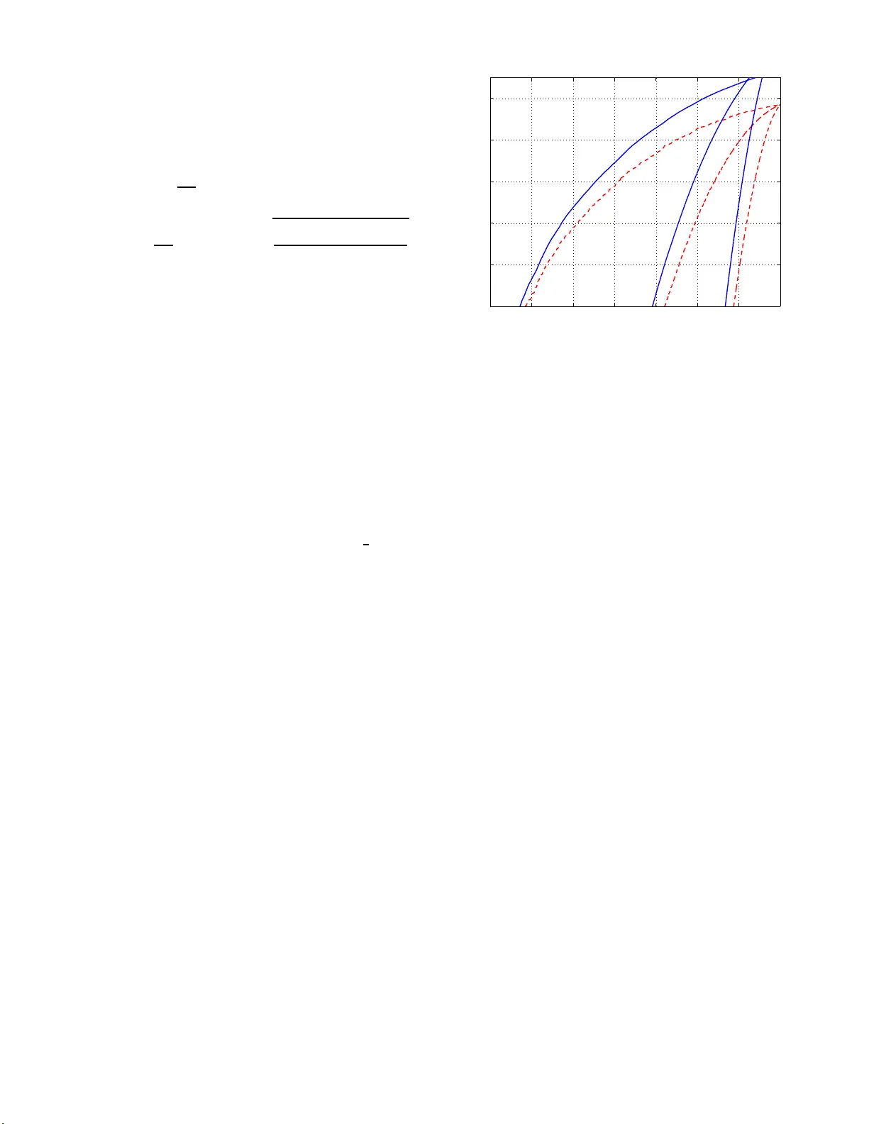
1 Channel polarizat ion: A method for constructing capacit y-achie ving cod es for s ymmetric binary-input memoryless channels Erdal Arıkan, Senior Member , IEEE Abstract — A method is propose d, called channel polarization, to construct code sequences that achiev e the symmetric capacity I ( W ) of any giv en binary-inpu t discrete memoryless channel (B- DMC) W . The symmetric capacity is th e hi ghest rate achiev able subject to using the input letters of the channel with equal probability . Channel polarization r efers to the fac t that it is possible to synthesize, out of N independen t copies of a given B-DMC W , a seco nd set of N bi nary-input channels { W ( i ) N : 1 ≤ i ≤ N } su ch that, as N becomes large, the fraction of indices i fo r which I ( W ( i ) N ) is near 1 approaches I ( W ) and the fraction f or which I ( W ( i ) N ) i s near 0 approaches 1 − I ( W ) . The polarized channels { W ( i ) N } are well-conditioned for channel coding: o ne need only send data at rate 1 thr ough th ose with capacity near 1 and at rate 0 through the remaining. Codes constructed on t he basis of this id ea are called polar codes. The paper pro ves that, given any B-DMC W with I ( W ) > 0 and any target rate R < I ( W ) , there exists a sequence of polar codes { C n ; n ≥ 1 } such that C n has block-length N = 2 n , rate ≥ R , and probability of block error under successiv e cancellation decodin g bounded as P e ( N , R ) ≤ O ( N − 1 4 ) ind ependently of the code rate. This perf ormance is achie vable by encoders and decoders with complexity O ( N log N ) f or each. Index T erms — Capacity-achieving codes, channel capacity , channel polarization, Plotkin construction, polar codes, Reed- Muller codes, successiv e cancellation decoding. I . I N T RO D U C T I O N A N D OV E RV I E W A f ascinating aspect of Shanno n’ s p roof of the noisy channel coding th eorem is the random- coding m ethod th at he used to show the existence of capacity-achieving c ode sequen ces without exhibiting any speciﬁc such sequ ence [1]. Explicit construction of provably cap acity-achieving code sequenc es with lo w en coding and decodin g co mplexities has since then been an elusive goal. This pap er is an attempt to meet this goal for th e class o f B-DMCs. W e will give a description of the main ideas and results of the paper in this section. First, we give so me deﬁnitions an d state some basic facts that are used th rough out the p aper . A. Pr eliminaries W e write W : X → Y to denote a ge neric B-DMC with in put alphabet X , ou tput alph abet Y , an d tran sition E. Arık an is with th e Department of E lectri cal-Elec tronics Engineer ing, Bilk ent Unive rsity , Ankara, 06800, T urke y (e-mail: arikan@e e.bilk ent.edu .tr) This w ork was suppo rted in part by The Scientiﬁc and T e chnolog ical Researc h Council of Turk ey (T UBIT AK) under Project 107E216 and in part by the Europ ean Commission FP7 Network of Exc ellen ce NEW COM++ un der contrac t 216715. probab ilities W ( y | x ) , x ∈ X , y ∈ Y . The input alphabet X will always be { 0 , 1 } , the o utput alph abet and the transition probab ilities may be arbitrar y . W e write W N to den ote the channel correspon ding to N uses of W ; thus, W N : X N → Y N with W N ( y N 1 | x N 1 ) = Q N i =1 W ( y i | x i ) . Giv en a B-DMC W , there are two channel parameter s of primary interest in this p aper: the sym metric capacity I ( W ) ∆ = X y ∈Y X x ∈X 1 2 W ( y | x ) log W ( y | x ) 1 2 W ( y | 0) + 1 2 W ( y | 1) and the Bhattach aryya param eter Z ( W ) ∆ = X y ∈Y p W ( y | 0) W ( y | 1) . These para meters are used as measures o f rate and reliability , respectively . I ( W ) is the h ighest rate at which reliable com- munication is p ossible across W using the inputs of W with equal f requen cy . Z ( W ) is an upp er bo und on the pro bability of m aximum- likelihood (ML) decision error when W is u sed only once to transmit a 0 or 1. It is easy to see that Z ( W ) takes values in [0 , 1] . Throu gh- out, we will u se base- 2 logar ithms; hence, I ( W ) will also take values in [0 , 1] . The unit for code rates and channe l capa cities will be bits . Intuitively , one would exp ect that I ( W ) ≈ 1 iff Z ( W ) ≈ 0 , and I ( W ) ≈ 0 if f Z ( W ) ≈ 1 . The following boun ds, proved in the Ap pendix , make this pr ecise. Pr oposition 1: For any B-DMC W , we ha ve I ( W ) ≥ lo g 2 1 + Z ( W ) , (1) I ( W ) ≤ p 1 − Z ( W ) 2 . (2) The symmetric capacity I ( W ) equals the Shannon capac ity when W is a symmetric channel, i.e ., a chan nel fo r which there exists a per mutation π of th e outp ut alphabet Y such that (i) π − 1 = π and (ii) W ( y | 1) = W ( π ( y ) | 0) fo r all y ∈ Y . The binary symmetric channel (BSC) and the binary erasure channel (BEC) are examples of symme tric channels. A BSC is a B-DMC W with Y = { 0 , 1 } , W (0 | 0) = W (1 | 1 ) , and W (1 | 0) = W (0 | 1) . A B-DMC W is called a BEC if for each y ∈ Y , either W ( y | 0) W ( y | 1) = 0 or W ( y | 0 ) = W ( y | 1) . In the latter case, y is said to be an erasure symbol. The s um of W ( y | 0) over all erasure symb ols y is called the erasur e probab ility of the BEC. 2 W e d enote ran dom variables (R Vs) by up per-case letters, such as X , Y , and th eir realizations (sam ple values) by the correspo nding lower-case letters, such as x , y . For X a R V , P X denotes the pr obability assignme nt on X . For a join t ensem ble of R Vs ( X , Y ) , P X,Y denotes the join t probability assignment. W e use the standard no tation I ( X ; Y ) , I ( X ; Y | Z ) to denote the mutual infor mation an d its con ditional fo rm, respectively . W e use the notation a N 1 as shorthand for denoting a ro w vector ( a 1 , . . . , a N ) . Giv e n such a vector a N 1 , we write a j i , 1 ≤ i, j ≤ N , to denote the s ubvector ( a i , . . . , a j ) ; if j < i , a j i is regarded as v o id. Giv en a N 1 and A ⊂ { 1 , . . . , N } , we write a A to den ote the subvector ( a i : i ∈ A ) . W e write a j 1 ,o to den ote the subv ec tor with odd indices ( a k : 1 ≤ k ≤ j ; k odd ) . W e write a j 1 ,e to denote the subvector with even indices ( a k : 1 ≤ k ≤ j ; k even ) . For example, for a 5 1 = (5 , 4 , 6 , 2 , 1 ) , we h av e a 4 2 = (4 , 6 , 2) , a 5 1 ,e = (4 , 2 ) , a 4 1 ,o = (5 , 6 ) . The notation 0 N 1 is used to d enote the all- zero vector . Code construction s in th is paper will be carried out in vector spaces over the bina ry ﬁeld GF(2). Unless speciﬁed otherwise, all vectors, matrices, and op erations on them will b e over GF(2). In p articular, f or a N 1 , b N 1 vectors over GF(2) , we write a N 1 ⊕ b N 1 to d enote their compon entwise mo d-2 sum. The Kronecker prod uct of an m -by- n matrix A = [ A ij ] and an r -b y- s matrix B = [ B ij ] is deﬁned as A ⊗ B =    A 11 B · · · A 1 n B . . . . . . . . . A m 1 B · · · A mn B    , which is an mr -by- ns matrix. The Kronecker p ower A ⊗ n is deﬁned as A ⊗ A ⊗ ( n − 1) for all n ≥ 1 . W e will follow th e conv en tion that A ⊗ 0 ∆ = [1] . W e write |A| to deno te the number of elemen ts in a set A . W e write 1 A to denote the indicator function of a set A ; thus, 1 A ( x ) equals 1 if x ∈ A and 0 other wise. W e use the stand ard Landau notatio n O ( N ) , o ( N ) , ω ( N ) to den ote the asymp totic b ehavior of functions. B. Channel polarization Channel polarization is an operation by w hich one manu- factures out of N in depend ent copies of a g iv e n B-DMC W a second s et of N channels { W ( i ) N : 1 ≤ i ≤ N } that show a polarization ef f ect in the sense that, as N beco mes large, the symm etric capacity ter ms { I ( W ( i ) N ) } tend towards 0 or 1 for all but a vanishing fraction o f indic es i . T his o peration consists of a chann el co mbining phase and a chann el splitting phase. 1) Channel combining : This phase comb ines c opies of a giv en B-DMC W in a recu rsiv e manner to produce a vector channel W N : X N → Y N , where N c an be any power of two, N = 2 n , n ≥ 0 . The re cursion begins at the 0- th level ( n = 0 ) with o nly on e copy of W and we set W 1 ∆ = W . The ﬁrst level ( n = 1 ) of the recu rsion co mbines two indep endent copies o f W 1 as shown in Fig. 1 and obtain s the channel W 2 : X 2 → Y 2 with the tra nsition pro babilities W 2 ( y 1 , y 2 | u 1 , u 2 ) = W ( y 1 | u 1 ⊕ u 2 ) W ( y 2 | u 2 ) . (3) + W W u 2 u 1 x 2 x 1 y 2 y 1 W 2 Fig. 1. The channel W 2 . The next level of the recursion is shown in Fig. 2 where two indepen dent cop ies of W 2 are comb ined to create the c hannel W 4 : X 4 → Y 4 with transition prob abilities W 4 ( y 4 1 | u 4 1 ) = W 2 ( y 2 1 | u 1 ⊕ u 2 , u 3 ⊕ u 4 ) W 2 ( y 4 3 | u 2 , u 4 ) . + W W x 4 x 3 y 4 y 3 W 2 + W W x 2 x 1 y 2 y 1 W 2 + + W 4 v 2 v 1 v 4 v 3 u 1 u 2 u 3 u 4 R 4 Fig. 2. The channel W 4 and its relation to W 2 and W . In Fig. 2, R 4 is the permutation operation that maps an in put ( s 1 , s 2 , s 3 , s 4 ) to v 4 1 = ( s 1 , s 3 , s 2 , s 4 ) . The mapp ing u 4 1 7→ x 4 1 from the input of W 4 to th e inpu t o f W 4 can be written as x 4 1 = u 4 1 G 4 with G 4 =  1 0 0 0 1 0 1 0 1 1 0 0 1 1 1 1  . Thus, we have the relation W 4 ( y 4 1 | u 4 1 ) = W 4 ( y 4 1 | u 4 1 G 4 ) betwe en the transition probab ilities of W 4 and those o f W 4 . The general form of the recursion is shown in Fig. 3 whe re two in depend ent copie s o f W N/ 2 are comb ined to produ ce the channel W N . The input vector u N 1 to W N is ﬁrst tr ansforme d into s N 1 so that s 2 i − 1 = u 2 i − 1 ⊕ u 2 i and s 2 i = u 2 i for 1 ≤ i ≤ N / 2 . The op erator R N in the ﬁgure is a permutatio n, known as the reverse shufﬂe operation , and acts on its input s N 1 to prod uce v N 1 = ( s 1 , s 3 , . . . , s N − 1 , s 2 , s 4 , . . . , s N ) , which becomes the input to th e two cop ies of W N/ 2 as sho w n in the ﬁgure. W e observe that th e mapp ing u N 1 7→ v N 1 is linear over GF(2). It follows by ind uction th at the overall m apping u N 1 7→ x N 1 , from the inpu t of the synthesized chan nel W N to the input of the und erlying raw c hannels W N , is also linear and may be represented by a matrix G N so that x N 1 = u N 1 G N . W e call G N 3 W N R N W N/ 2 W N/ 2 u 1 s 1 + v 1 y 1 u 2 s 2 v 2 y 2 u N/ 2 − 1 s N/ 2 − 1 + v N/ 2 − 1 y N/ 2 − 1 u N/ 2 s N/ 2 v N/ 2 y N/ 2 u N/ 2+1 s N/ 2+1 + v N/ 2+1 y N/ 2+1 u N/ 2+2 s N/ 2+2 v N/ 2+2 y N/ 2+2 u N − 1 s N − 1 + v N − 1 y N − 1 u N s N v N y N . . . . . . . . . . . . . . . . . . . . . . . . Fig. 3. Recursi ve constru ction of W N from two copie s of W N/ 2 . the generato r matrix of size N . Th e tran sition pro babilities of the two chann els W N and W N are relate d by W N ( y N 1 | u N 1 ) = W N ( y N 1 | u N 1 G N ) (4) for all y N 1 ∈ Y N , u N 1 ∈ X N . W e will show in Sect. VII that G N equals B N F ⊗ n for an y N = 2 n , n ≥ 0 , where B N is a permutatio n matrix kn own as bit-reversal and F ∆ = [ 1 0 1 1 ] . Note that th e cha nnel com bining operatio n is fu lly sp eciﬁed by the matrix F . Also note that G N and F ⊗ n have the same set of rows, but in a different (b it-reversed) order; we will discuss this topic m ore fully in Sect. VI I. 2) Channel splittin g : Having synthesized the vector ch an- nel W N out of W N , the next step o f channe l polarization is to split W N back into a set of N binary -input coordina te channels W ( i ) N : X → Y N × X i − 1 , 1 ≤ i ≤ N , d eﬁned by the transition pro babilities W ( i ) N ( y N 1 , u i − 1 1 | u i ) ∆ = X u N i +1 ∈X N − i 1 2 N − 1 W N ( y N 1 | u N 1 ) , (5) where ( y N 1 , u i − 1 1 ) d enotes the ou tput of W ( i ) N and u i its input. T o gain an in tuitiv e under standing of the chann els { W ( i ) N } , consider a genie- aided succe ssi ve cancellation deco der in which the i th decision element estimates u i after observ ing y N 1 and the past channel inputs u i − 1 1 (supplied correctly by the genie regard less of an y decision errors at earlier stages). If u N 1 is a-prio ri uniform on X N , then W ( i ) N is the effective channel seen b y the i th decision elemen t in this scenario. 3) Cha nnel po la rization: Theor e m 1 : For any B-DMC W , the channels { W ( i ) N } polarize in the sense th at, for any ﬁxed δ ∈ (0 , 1 ) , as N goes to inﬁnity thro ugh powers of two, the frac tion o f indice s i ∈ { 1 , . . . , N } fo r wh ich I ( W ( i ) N ) ∈ (1 − δ, 1] goes to I ( W ) and the frac tion for which I ( W ( i ) N ) ∈ [0 , δ ) goes to 1 − I ( W ) . This theorem is proved in Sect. IV. 1 256 512 768 1024 0 0.1 0.2 0.3 0.4 0.5 0.6 0.7 0.8 0.9 1 Channel index Symmetric capacity Fig. 4. Plot of I ( W ( i ) N ) vs. i = 1 , . . . , N = 2 10 for a BEC with ǫ = 0 . 5 . The polar ization effect is illustrated in Fig. 4 for the case W is a B EC with er asure probab ility ǫ = 0 . 5 . The numb ers { I ( W ( i ) N ) } have be en comp uted using the r ecursive relations I ( W (2 i − 1) N ) = I ( W ( i ) N/ 2 ) 2 , I ( W (2 i ) N ) = 2 I ( W ( i ) N/ 2 ) − I ( W ( i ) N/ 2 ) 2 , (6) with I ( W (1) 1 ) = 1 − ǫ . This recursion is v a lid only fo r BECs and it is proved in Sect. III. No efﬁcient alg orithm is kn own for calculatio n o f { I ( W ( i ) N ) } for a ge neral B-DMC W . Figure 4 shows that I ( W ( i ) ) tend s to be n ear 0 fo r small i and near 1 fo r large i . Howe ver , I ( W ( i ) N ) shows an erratic behavior for an in termediate range o f i . For gener al B-DMCs, determinin g the subset of ind ices i for which I ( W ( i ) N ) is above a given thresho ld is an important comp utational p roblem that will be add ressed in Sect. IX. 4) Ra te of p olarization: For provin g co ding the orems, the speed with which the po larization effect takes hold as a function of N is im portant. Our main result in this regard is given in term s of the p arameters Z ( W ( i ) N ) = X y N 1 ∈Y N X u i − 1 1 ∈X i − 1 q W ( i ) N ( y N 1 , u i − 1 1 | 0) W ( i ) N ( y N 1 , u i − 1 1 | 1) . (7) Theor e m 2 : For any B-DMC W with I ( W ) > 0 , and any ﬁxed R < I ( W ) , th ere exists a sequen ce of sets A N ⊂ { 1 , . . . , N } , N ∈ { 1 , 2 , . . . , 2 n , . . . } , such that |A N | ≥ N R and Z ( W ( i ) N ) ≤ O ( N − 5 / 4 ) for all i ∈ A N . This theorem is proved in Sect. IV -B. 4 W e stated the po larization r esult in Theo rem 2 in terms { Z ( W ( i ) N ) } rather than { I ( W ( i ) N ) } because this for m is better suited to the codin g results that we will de velo p. A rate of polarization result in te rms of { I ( W ( i ) N ) } can be ob tained from Theorem 2 with the help of Pro p. 1. C. P olar codin g W e take advantage of the polar ization effect to construct codes that achieve the symmetric channel capacity I ( W ) by a meth od we call po lar coding . The basic id ea o f p olar coding is to create a co ding system where on e can acc ess each coord inate chan nel W ( i ) N individually an d send data only throug h those for wh ich Z ( W ( i ) N ) is near 0 . 1) G N -coset code s: W e ﬁrst describe a class of block codes that con tain polar code s—the codes of m ain inter est—as a special case. T he block -lengths N for this class are restricted to powers of two, N = 2 n for some n ≥ 0 . For a gi ven N , each cod e in the class is encoded in th e same man ner, namely , x N 1 = u N 1 G N (8) where G N is the generato r m atrix of ord er N , deﬁned above. For A an arb itrary subset of { 1 , . . . , N } , we may wr ite (8) as x N 1 = u A G N ( A ) ⊕ u A c G N ( A c ) (9) where G N ( A ) denotes the submatrix o f G N formed by the rows with indices in A . If we no w ﬁx A and u A c , but leave u A as a free variable, we o btain a m apping from source b locks u A to codeword blocks x N 1 . This m apping is a coset co de : it is a coset of the linear block code with generato r matrix G N ( A ) , with the coset determined by the ﬁxed vector u A c G N ( A c ) . W e will refer to this class o f codes c ollectively as G N -coset codes . Individual G N -coset codes will b e iden tiﬁed by a para meter vector ( N , K , A , u A c ) , where K is the code dimensio n and speciﬁes the size of A . 1 The ratio K / N is called the code rate . W e will ref er to A as the informa tion set and to u A c ∈ X N − K as frozen bits or vector . For examp le, the (4 , 2 , { 2 , 4 } , (1 , 0)) cod e has the encoder mapping x 4 1 = u 4 1 G 4 = ( u 2 , u 4 )  1 0 1 0 1 1 1 1  + (1 , 0)  1 0 0 0 1 1 0 0  . (10) For a sour ce block ( u 2 , u 4 ) = (1 , 1 ) , the cod ed block is x 4 1 = (1 , 1 , 0 , 1) . Polar co des will be speciﬁed sho rtly by gi vin g a particular rule for th e selection o f the info rmation set A . 2) A successive cancellatio n deco der: Consider a G N -coset code with par ameter ( N , K, A , u A c ) . Let u N 1 be encoded into a codeword x N 1 , let x N 1 be sent over the channel W N , and let a ch annel outpu t y N 1 be received. The de coder’ s task is to generate an estimate ˆ u N 1 of u N 1 , given knowledge of A , u A c , and y N 1 . Since the d ecoder can avoid erro rs in the frozen p art 1 W e include the redund ant parameter K in the paramete r s et because often we consider an ensemble of codes with K ﬁxed and A free. by setting ˆ u A c = u A c , the real decoding task is to g enerate an estimate ˆ u A of u A . The co ding results in this p aper will be given with respect to a speciﬁc successive can cellation (SC) deco der, unless some other deco der is mentioned. Giv en any ( N , K , A , u A c ) G N - coset code, we will use a SC decoder that generates its decision ˆ u N 1 by comp uting ˆ u i ∆ = ( u i , if i ∈ A c h i ( y N 1 , ˆ u i − 1 1 ) , if i ∈ A (11) in the order i fro m 1 to N , where h i : Y N × X i − 1 → X , i ∈ A , are decision functio ns deﬁned as h i ( y N 1 , ˆ u i − 1 1 ) ∆ =    0 , if W ( i ) N ( y N 1 , ˆ u i − 1 1 | 0) W ( i ) N ( y N 1 , ˆ u i − 1 1 | 1) ≥ 1 1 , otherwise (12) for all y N 1 ∈ Y N , ˆ u i − 1 1 ∈ X i − 1 . W e will say that a deco der block error occurre d if ˆ u N 1 6 = u N 1 or equ iv alently if ˆ u A 6 = u A . The decision f unctions { h i } deﬁned ab ove resemble ML decision functions but are not exactly so, because th ey treat the future frozen bits ( u j : j > i , j ∈ A c ) as R Vs, rather than as known bits. I n exchang e for this suboptimality , { h i } can b e computed efﬁciently using r ecursive formulas, as we will show in Sect. II. Apart from algorithmic efﬁcienc y , th e recursive structure of th e decision functions is impor tant becau se it renders th e p erform ance ana lysis of the d ecoder tractab le. Fortunately , the loss in perfo rmance d ue to no t using true ML decision function s happens to be negligible: I ( W ) is still achiev ab le. 3) Cod e performanc e: The notation P e ( N , K, A , u A c ) will denote the proba bility of b lock error for a ( N , K , A , u A c ) code, assuming tha t each da ta vector u A ∈ X K is sent with pr obability 2 − K and d ecoding is done by the ab ove SC decoder . More p recisely , P e ( N , K, A , u A c ) ∆ = X u A ∈X K 1 2 K X y N 1 ∈Y N : ˆ u N 1 ( y N 1 ) 6 = u N 1 W N ( y N 1 | u N 1 ) . The av erage of P e ( N , K, A , u A c ) over all choices for u A c will be deno ted b y P e ( N , K, A ) : P e ( N , K, A ) ∆ = X u A c ∈X N − K 1 2 N − K P e ( N , K, A , u A c ) . A key b ound on block erro r p robab ility u nder SC decod ing is the f ollowing. Pr oposition 2: For any B-DMC W and any choice of the parameters ( N , K , A ) , P e ( N , K, A ) ≤ X i ∈A Z ( W ( i ) N ) . (13) Hence, for each ( N , K, A ) , there exists a frozen vector u A c such that P e ( N , K, A , u A c ) ≤ X i ∈A Z ( W ( i ) N ) . (14) This is pr oved in Sect. V -B. This result sug gests choosing A from amo ng all K - subsets of { 1 , . . . , N } so as to min imize 5 the RHS of (13). T his id ea leads to the deﬁnition of polar codes. 4) P olar co des: Gi ven a B-DMC W , a G N -coset c ode with parameter ( N , K, A , u A c ) will be called a polar c ode for W if the inform ation s et A is chosen as a K - element subset of { 1 , . . . , N } such tha t Z ( W ( i ) N ) ≤ Z ( W ( j ) N ) for all i ∈ A , j ∈ A c . Polar co des are channel-speciﬁc design s: a po lar co de for one chan nel may no t be a polar code for anothe r . T he main result of this paper will be to show that polar coding achieves the symm etric c apacity I ( W ) of a ny given B-DMC W . An altern ativ e r ule fo r polar code deﬁnition would b e to specify A as a K -elemen t subset of { 1 , . . . , N } such that I ( W ( i ) N ) ≥ I ( W ( j ) N ) for all i ∈ A , j ∈ A c . T his alternati ve rule would also ach ieve I ( W ) . Howe ver , the ru le based on the Bhattachary ya par ameters has the advantage o f being connected with an explicit bo und o n block er ror prob ability . The polar c ode deﬁnition does not specify how the frozen vector u A c is to be ch osen; it may be chosen at will. Th is degree o f f reedom in the choice o f u A c simpliﬁes the perfo r- mance analy sis o f polar codes by allo wing averaging over an ensemble. However , it is n ot f or analytical conv e nience alone that we do not specify a precise rule for selecting u A c , b u t also because it a ppears that the cod e pe rforma nce is r elativ e ly insensitiv e to th at ch oice. In fact, we prove in Sect. VI-B that, for symmetric channels, any choice for u A c is as goo d a s any other . 5) Coding theor e m s: Fix a B-DM C W and a nu mber R ≥ 0 . Let P e ( N , R ) be deﬁne d as P e ( N , ⌊ N R ⌋ , A ) with A selected in accor dance with the polar cod ing rule for W . Thus, P e ( N , R ) is the prob ability o f block error under SC decodin g for polar coding over W with block-length N and rate R , av er aged over all choices fo r the froze n bits u A c . The main codin g r esult of th is paper is the fo llowing: Theor e m 3 : For any g i ven B-DMC W an d ﬁxed R < I ( W ) , block error p robab ility fo r polar coding u nder succ es- si ve can cellation deco ding satisﬁes P e ( N , R ) = O ( N − 1 4 ) . (15) This the orem follows as a n easy corollar y to Th eorem 2 an d the b ound (13), as we show in Sect. V -B. For symmetric chan - nels, we have th e fo llowing stronge r version of Th eorem 3. Theor e m 4 : For any symmetric B-DMC W an d any ﬁxed R < I ( W ) , consider any sequence o f G N -coset codes ( N , K, A , u A c ) with N increasing to in ﬁnity , K = ⌊ N R ⌋ , A ch osen in acc ordanc e with the po lar coding r ule for W , and u A c ﬁxed arbitrarily . The block error pr obability under successiv e can cellation decod ing satisﬁes P e ( N , K, A , u A c ) = O ( N − 1 4 ) . (16) This is proved in Sect. VI-B. Note th at for symm etric channels I ( W ) equals the Shannon capa city of W . 6) Complexity: An important issue about polar coding is the co mplexity of enc oding, decod ing, and co de con struction. The recursi ve structure of the channel po larization co nstruction leads to low-complexity encoding and deco ding algorithms for the class o f G N -coset c odes, and in par ticular, for polar co des. Theor e m 5 : For the cla ss of G N -coset cod es, the complex- ity of enco ding and the co mplexity of successive cancellation decodin g are b oth O ( N log N ) as function s of code blo ck- length N . This theo rem is p roved in Sections VII and VIII. Notice that the c omplexity bo unds in Theorem 5 are ind ependen t of the code rate and the way the frozen vector is chosen. The bound s hold ev en at r ates above I ( W ) , but clearly this h as no practical signiﬁcan ce. As f or cod e co nstruction , we h ave found no low-complexity algorithm s for c onstructing polar co des. One exception is th e case o f a BEC for which we have a polar cod e con struc- tion algorithm with complexity O ( N ) . W e d iscuss the code construction pr oblem fu rther in Sect. IX and sug gest a lo w- complexity statistical algo rithm for approx imating the exact polar code con struction. D. Relations to pre v io us work This paper is an extension of work b egun in [2], whe re channel co mbinin g and splitting were used to show th at improvements can be obta ined in th e sum cutoff rate for som e speciﬁc DMCs. Howe ver, no r ecursive m ethod was sugg ested there to reach the u ltimate limit o f such impr ovements. As the present work progressed, it be came clea r that polar coding had much in c ommon with Reed -Muller (RM) coding [3], [4]. Indeed , r ecursive code construction a nd SC deco ding, which are two essential ing redients of polar cod ing, appear to have been introd uced into cod ing theory by RM codes. According to one construction of RM cod es, for any N = 2 n , n ≥ 0 , and 0 ≤ K ≤ N , an RM cod e w ith block - length N an d dimen sion K , denoted RM ( N , K ) , is deﬁned as a linear co de wh ose g enerator matrix G RM ( N , K ) is obtained by deleting ( N − K ) of the rows of F ⊗ n so that n one of the deleted ro ws has a larger Hamm ing we ight (n umber of 1s in that row) than any of the r emaining K rows. For in stance, G RM (4 , 4) = F ⊗ 2 =  1 0 0 0 1 1 0 0 1 0 1 0 1 1 1 1  and G RM (4 , 2) = [ 1 0 1 0 1 1 1 1 ] . This con struction brings out the similarities betwee n RM codes an d po lar cod es. Since G N and F ⊗ n have the same set of rows (o nly in a different or der) for any N = 2 n , it is clear that RM codes belong to the class o f G N -coset codes. For example, RM (4 , 2) is the G 4 -coset co de with parameter (4 , 2 , { 2 , 4 } , (0 , 0)) . So , RM coding and polar coding may be regarded as two alter native rules for selecting the infor mation set A of a G N -coset cod e of a given size ( N , K ) . Unlike po lar coding, RM codin g selects the info rmation set in a ch annel- indepen dent manner; it is n ot as ﬁne-tune d to the cha nnel polarization pheno menon as polar cod ing is. W e will show in Sect. X that, at least for the class of B ECs, the RM rule for inf ormation set selection lead s to asy mptotically u nreliable codes under SC deco ding. So , polar codin g g oes beyond RM coding in a non -trivial manner by p aying closer attention to channel polariz ation. Another con nection to existing work can be established by noting that polar cod es are multi-level | u | u + v | co des, which are a class of codes originating from Plotk in’ s method for code com bining [5]. This con nection is not surprising in 6 view of the fact th at RM co des are also m ulti-level | u | u + v | codes [6, pp. 114-1 25]. Howev e r , u nlike ty pical multi-level code construc tions where one begins with speciﬁc small codes to b u ild larger on es, in polar co ding the multi-le vel code is obtained by expurgating rows o f a full-or der genera tor m atrix, G N , with respect to a channel- speciﬁc criterion. The special structure of G N ensures that, no matter how expurgatio n is done, the resulting cod e is a multi-level | u | u + v | code. In essence, p olar cod ing en joys th e fr eedom to pick a mu lti-lev el code from an ensemble of su ch code s so as to suit the channe l at hand, wh ile co n ventional approac hes to multi-level cod ing do not h av e th is degree of ﬂexibility . Finally , we wish to mention a “spe ctral” in terpretation o f p o- lar co des which is similar to Blahut’ s treatment of BCH codes [7, Ch. 9 ]; th is ty pe of similarity has already b een p ointed o ut by Forney [8, Ch. 11 ] in connection with RM codes. From the spe ctral v iewpoint, th e encodin g operation ( 8) is regarded as a transfor m of a “ frequen cy” d omain informatio n vector u N 1 to a “time” domain codew o rd vector x N 1 . The transfo rm is in vertible with G − 1 N = G N . Th e d ecoding o peration is regarded as a spectral estimation problem in which one is giv en a time domain observation y N 1 , which is a noisy version of x N 1 , and asked to estimate u N 1 . T o aid the estima tion task, o ne is allowed to f reeze a cer tain n umber of spectral comp onents of u N 1 . This spec tral interp retation o f p olar codin g suggests that it may be possible to tre at polar codes and BCH code s in a uniﬁed frame work . The spectral in terpretation also op ens the door to the use of various s ig nal processing techniqu es in polar coding; indeed , in Sect. VII, we exploit some fast transform technique s in designing en coders for po lar co des. E. P aper outline The rest of the paper is organized as follows. Sect. II explores the recur si ve properties of the channel splitting op- eration. In Sect. III, we focus on how I ( W ) an d Z ( W ) get transform ed through a single step of chan nel combining and splitting. W e extend this to an asymptotic analysis in Sect. IV and complete the p roofs of Theorem 1 and Theor em 2. This completes the part of the p aper on channel p olarization; th e rest of the p aper is mainly abou t polar c oding. Section V develops an upp er bound on the block error p robab ility of polar coding under SC d ecoding and p roves Theore m 3 . Sect. VI considers polar coding for symmetr ic B-DMCs and proves Theorem 4. Sect. VII gives an a nalysis of the encod er mapping G N , which results in efﬁcient encoder implemen tations. In Sect. VIII, we give an imp lementation of SC decod ing with complexity O ( N log N ) . In Sect. IX, we discuss the c ode construction complexity and propo se an O ( N lo g N ) statistical algorithm for approx imate code construction. In Sect. X, we explain why RM codes have a poor asymptotic perform ance under SC d ecoding . In Sect. XI, we poin t out some gen eraliza- tions of the p resent work, giv e some com plementar y remar ks, and state som e open p roblems. I I . R E C U R S I V E C H A N N E L T R A N S F O R M A T I O N S W e ha ve deﬁned a blockwise channel combinin g and split- ting operation by (4) and (5) which transformed N indepen- dent copies of W in to W (1) N , . . . , W ( N ) N . The goal in this sec- tion is to show tha t this blo ckwise chan nel tr ansformatio n c an be bro ken recursi vely into single- step channel transfo rmations. W e say that a pair of binary-in put ch annels W ′ : X → ˜ Y and W ′′ : X → ˜ Y × X are obtained by a single-step transform ation of two indep endent co pies of a binary- input channel W : X → Y and write ( W , W ) 7→ ( W ′ , W ′′ ) iff there exists a one-to-one mapping f : Y 2 → ˜ Y such that W ′ ( f ( y 1 , y 2 ) | u 1 ) = X u ′ 2 1 2 W ( y 1 | u 1 ⊕ u ′ 2 ) W ( y 2 | u ′ 2 ) , (17) W ′′ ( f ( y 1 , y 2 ) , u 1 | u 2 ) = 1 2 W ( y 1 | u 1 ⊕ u 2 ) W ( y 2 | u 2 ) (18) for all u 1 , u 2 ∈ X , y 1 , y 2 ∈ Y . According to this, we can write ( W, W ) 7→ ( W (1) 2 , W (2) 2 ) for any given B-DMC W becau se W (1) 2 ( y 2 1 | u 1 ) ∆ = X u 2 1 2 W 2 ( y 2 1 | u 2 1 ) = X u 2 1 2 W ( y 1 | u 1 ⊕ u 2 ) W ( y 2 | u 2 ) , (19) W (2) 2 ( y 2 1 , u 1 | u 2 ) ∆ = 1 2 W 2 ( y 2 1 | u 2 1 ) = 1 2 W ( y 1 | u 1 ⊕ u 2 ) W ( y 2 | u 2 ) , (20) which are in the form of (17) and (18) by taking f as th e identity map ping. It turn s out we can write, mo re genera lly , ( W ( i ) N , W ( i ) N ) 7→ ( W (2 i − 1) 2 N , W (2 i ) 2 N ) . (21) This follows as a corollary to the following: Pr oposition 3: For any n ≥ 0 , N = 2 n , 1 ≤ i ≤ N , W (2 i − 1) 2 N ( y 2 N 1 , u 2 i − 2 1 | u 2 i − 1 ) = X u 2 i 1 2 W ( i ) N ( y N 1 , u 2 i − 2 1 ,o ⊕ u 2 i − 2 1 ,e | u 2 i − 1 ⊕ u 2 i ) · W ( i ) N ( y 2 N N + 1 , u 2 i − 2 1 ,e | u 2 i ) (22 ) and W (2 i ) 2 N ( y 2 N 1 , u 2 i − 1 1 | u 2 i ) = 1 2 W ( i ) N ( y N 1 , u 2 i − 2 1 ,o ⊕ u 2 i − 2 1 ,e | u 2 i − 1 ⊕ u 2 i ) · W ( i ) N ( y 2 N N + 1 , u 2 i − 2 1 ,e | u 2 i ) . (23 ) This pr oposition is pr oved in the Ap pendix. The tr ansform relationship (21) can no w be justiﬁed by noting that (2 2) and (23) are identical in form to (1 7) and ( 18), respectively , after the following sub stitutions: W ← W ( i ) N , W ′ ← W (2 i − 1) 2 N , W ′′ ← W (2 i ) 2 N , u 1 ← u 2 i − 1 , u 2 ← u 2 i , y 1 ← ( y N 1 , u 2 i − 2 1 ,o ⊕ u 2 i − 2 1 ,e ) , y 2 ← ( y 2 N N + 1 , u 2 i − 2 1 ,e ) , f ( y 1 , y 2 ) ← ( y 2 N 1 , u 2 i − 2 1 ) . 7 W W W W W W W W W (2) 2 W (1) 2 W (2) 2 W (1) 2 W (2) 2 W (1) 2 W (2) 2 W (1) 2 W (4) 4 W (2) 4 W (3) 4 W (1) 4 W (4) 4 W (2) 4 W (3) 4 W (1) 4 W (8) 8 W (4) 8 W (6) 8 W (2) 8 W (7) 8 W (3) 8 W (5) 8 W (1) 8 Fig. 5. The channel transformation proce s s with N = 8 channe ls. Thus, we have shown that the blo ckwise c hannel tran s- formation from W N to ( W (1) N , . . . , W ( N ) N ) breaks at a local lev el into single- step channel transfo rmations of the f orm (21). The full set of such tran sformation s form a fabric as shown in Fig. 5 for N = 8 . Reading from rig ht to left, the ﬁgure starts with fou r c opies of th e tra nsformatio n ( W, W ) 7→ ( W (1) 2 , W (2) 2 ) and continues in b utterﬂy patterns, each repre- senting a ch annel tra nsformatio n o f th e form ( W ( j ) 2 i , W ( j ) 2 i ) 7→ ( W (2 j − 1) 2 i +1 , W (2 j ) 2 i +1 ) . The two ch annels at the r ight end-po ints of the butterﬂies are always identical an d ind ependen t. At the rightm ost level there a re 8 independ ent cop ies of W ; at the next level to the left, there are 4 independ ent copies of W (1) 2 and W (2) 2 each; and so o n. E ach step to the left doubles the number of ch annel types, b u t halves the nu mber of indep endent c opies. I I I . T R A N S F O R M A T I O N O F R AT E A N D R E L I A B I L I T Y W e now in vestigate h ow the r ate and reliability par ameters, I ( W ( i ) N ) and Z ( W ( i ) N ) , change thr ough a lo cal ( single-step) transform ation (21). By understand ing the loca l b ehavior , we will be able to re ach co nclusions about the ov e rall tran sfor- mation from W N to ( W (1) N , . . . , W ( N ) N ) . Proofs of th e re sults in this s ection are given in the Ap pendix . A. Local transformation of rate and r eliab ility Pr oposition 4: Sup pose ( W, W ) 7→ ( W ′ , W ′′ ) for some set of binar y-inpu t channe ls. Then , I ( W ′ ) + I ( W ′′ ) = 2 I ( W ) , (24) I ( W ′ ) ≤ I ( W ′′ ) (25) with equ ality iff I ( W ) equals 0 or 1 . The equ ality (24) indica tes that th e single-step channel transform preserves th e symmetric capacity . The inequ ality (25) together with (24) implies th at the symmetric capacity remains unchan ged u nder a single-step transfor m, I ( W ′ ) = I ( W ′′ ) = I ( W ) , iff W is either a perfect channel or a completely noisy o ne. If W is neith er perfec t no r completely noisy , th e sing le-step transfo rm moves th e symmetric capacity away from the center in the sense that I ( W ′ ) < I ( W ) < I ( W ′′ ) , th us helping polar ization. Pr oposition 5: Sup pose ( W, W ) 7→ ( W ′ , W ′′ ) for some set of binar y-inpu t channe ls. Then , Z ( W ′′ ) = Z ( W ) 2 , (26) Z ( W ′ ) ≤ 2 Z ( W ) − Z ( W ) 2 , (27) Z ( W ′ ) ≥ Z ( W ) ≥ Z ( W ′′ ) . (28) Equality holds in (27) if f W is a BEC. W e hav e Z ( W ′ ) = Z ( W ′′ ) if f Z ( W ) equals 0 or 1, or equiv alen tly , if f I ( W ) equals 1 or 0. This result shows that reliab ility can only improve u nder a single-step chan nel tr ansform in the sense that Z ( W ′ ) + Z ( W ′′ ) ≤ 2 Z ( W ) (29) with equality iff W is a BEC. Since th e BEC plays a special role w .r .t. extrem al behavior of reliability , it deserves special attention. Pr oposition 6: Consid er the channel transfor mation ( W , W ) 7→ ( W ′ , W ′′ ) . If W is a BEC with some erasure probab ility ǫ , then the chan nels W ′ and W ′′ are BECs with erasure pro babilities 2 ǫ − ǫ 2 and ǫ 2 , respec ti vely . Conv e rsely , if W ′ or W ′′ is a BEC, then W is BEC. B. Rate and reliability fo r W ( i ) N W e no w return to th e con text at th e end of Sect. II. Pr oposition 7: For any B-DMC W , N = 2 n , n ≥ 0 , 1 ≤ i ≤ N , the transfo rmation ( W ( i ) N , W ( i ) N ) 7→ ( W (2 i − 1) 2 N , W (2 i ) 2 N ) is rate-pr eserving and reliability- improving in th e sense that I ( W (2 i − 1) 2 N ) + I ( W (2 i ) 2 N ) = 2 I ( W ( i ) N ) , (30) Z ( W (2 i − 1) 2 N ) + Z ( W (2 i ) 2 N ) ≤ 2 Z ( W ( i ) N ) , (31) with eq uality in (31) iff W is a BEC. Chann el splitting moves the rate and reliability away f rom the center in the sense that I ( W (2 i − 1) 2 N ) ≤ I ( W ( i ) N ) ≤ I ( W (2 i ) 2 N ) , (32) Z ( W (2 i − 1) 2 N ) ≥ Z ( W ( i ) N ) ≥ Z ( W (2 i ) 2 N ) , (33) with equality in (3 2) and (33) if f I ( W ) equals 0 or 1. T he reliability terms fu rther satisfy Z ( W (2 i − 1) 2 N ) ≤ 2 Z ( W ( i ) N ) − Z ( W ( i ) N ) 2 , (34) Z ( W (2 i ) 2 N ) = Z ( W ( i ) N ) 2 , (35 ) with eq uality in (34) iff W is a BEC. The cumulative rate an d reliability satisfy N X i =1 I ( W ( i ) N ) = N I ( W ) , (36) N X i =1 Z ( W ( i ) N ) ≤ N Z ( W ) , (37) 8 with equ ality in (37) iff W is a B E C. This result follows from Prop. 4 and Pr op. 5 as a special case and n o separate pro of is needed . The cu mulative r elations (36) and (37) follow by repeated application of (3 0) and (31), respectively . The co nditions for eq uality in Prop . 4 are stated in terms o f W rather than W ( i ) N ; this is possible becau se: (i) by Prop. 4, I ( W ) ∈ { 0 , 1 } iff I ( W ( i ) N ) ∈ { 0 , 1 } ; and (ii) W is a BEC iff W ( i ) N is a BEC , which follo ws from Prop. 6 by induction . For the sp ecial case that W is a BEC with an erasure probab ility ǫ , it follows from Prop . 4 and Prop. 6 that th e parameters { Z ( W ( i ) N ) } can be com puted thro ugh the recur sion Z ( W (2 j − 1) N ) = 2 Z ( W ( j ) N/ 2 ) − Z ( W ( j ) N/ 2 ) 2 , Z ( W (2 j ) N ) = Z ( W ( j ) N/ 2 ) 2 , (38) with Z ( W (1) 1 ) = ǫ . The pa rameter Z ( W ( i ) N ) equa ls the erasure probab ility of the channel W ( i ) N . The recur si ve relations (6) follow from (38) by the fact tha t I ( W ( i ) N ) = 1 − Z ( W ( i ) N ) f or W a BEC. I V . C H A N N E L P O L A R I Z A T I O N W e prove the m ain re sults on channel p olarization in this section. The analysis is based on the recursive relationship s depicted in Fig. 5; howe ver, it will be more convenient to re- sketch Fig. 5 as a binary tree as shown in Fig. 6. The r oot node of the tree is ass o ciated with the ch annel W . Th e root W gi ves birth to an upp er chan nel W (1) 2 and a lower chann el W (2) 2 , whic h ar e associated with the two nodes at le vel 1. Th e channel W (1) 2 in turn gi ves birth to the chann els W (1) 4 and W (2) 4 , a nd so on. The channel W ( i ) 2 n is loca ted at le vel n of the tree at node nu mber i c ounting from the top. There is a natur al indexing of no des o f the tree in Fig. 6 by bit sequences. The root node i s indexed with the null sequence. The upp er node at le vel 1 is ind exed with 0 and the lower node with 1. Gi ven a node at le vel n with index b 1 b 2 · · · b n , the upper node emanating fro m it has the labe l b 1 b 2 · · · b n 0 and the lo wer node b 1 b 2 · · · b n 1 . According to th is labeling, the channel W ( i ) 2 n is situated at the node b 1 b 2 · · · b n with i = 1 + P n j =1 b j 2 n − j . W e d enote the ch annel W ( i ) 2 n located at nod e b 1 b 2 · · · b n alternatively as W b 1 ...b n . W e deﬁne a random tree process, denoted { K n ; n ≥ 0 } , in con nection with Fig. 6. The process begins at the ro ot of the tree with K 0 = W . For any n ≥ 0 , g iv en that K n = W b 1 ··· b n , K n +1 equals W b 1 ··· b n 0 or W b 1 ··· b n 1 with p robability 1/2 eac h. Thus, the path taken b y { K n } through the channel tree may be th ough t of as being d riven b y a sequ ence of i.i.d. Bernoulli R V s { B n ; n = 1 , 2 , . . . } where B n equals 0 or 1 with equ al probability . Gi ven that B 1 , . . . , B n has taken on a sample v alue b 1 , . . . , b n , the random ch annel process ta kes the v alue K n = W b 1 ··· b n . I n order to keep track of th e r ate and reliability param eters of the ran dom sequen ce of channels K n , we deﬁn e th e random pr ocesses I n = I ( K n ) and Z n = Z ( K n ) . For a more precise f ormula tion of the p roblem , we co nsider the prob ability space (Ω , F , P ) where Ω is th e space of all 0 1 W W (1) 2 = W 0 W (2) 2 = W 1 W (1) 4 = W 00 W (2) 4 = W 01 W (3) 4 = W 10 W (4) 4 = W 11 W (1) 8 = W 000 W (2) 8 = W 001 W (3) 8 = W 010 W (4) 8 = W 011 W (5) 8 = W 100 W (6) 8 = W 101 W (7) 8 = W 110 W (8) 8 = W 111 · · · · · · · · · · · · Fig. 6. The tree process for the recursi ve channel construction. binary sequences ( b 1 , b 2 , . . . ) ∈ { 0 , 1 } ∞ , F is the Borel ﬁeld (BF) generated by the cylinder s ets S ( b 1 , . . . , b n ) ∆ = { ω ∈ Ω : ω 1 = b 1 , . . . , ω n = b n } , n ≥ 1 , b 1 , . . . , b n ∈ { 0 , 1 } , and P is the probability measure d eﬁned on F such that P ( S ( b 1 , . . . , b n )) = 1 / 2 n . For each n ≥ 1 , we deﬁne F n as the BF generated by the c ylin der sets S ( b 1 , . . . , b i ) , 1 ≤ i ≤ n , b 1 , . . . , b i ∈ { 0 , 1 } . W e deﬁne F 0 as th e trivial BF c onsisting of the null set an d Ω o nly . Clearly , F 0 ⊂ F 1 ⊂ · · · ⊂ F . The ran dom processes describe d above can now be for mally deﬁned as f ollows. F o r ω = ( ω 1 , ω 2 , . . . ) ∈ Ω and n ≥ 1 , deﬁne B n ( ω ) = ω n , K n ( ω ) = W ω 1 ··· ω n , I n ( ω ) = I ( K n ( ω )) , and Z n ( ω ) = Z ( K n ( ω )) . For n = 0 , deﬁne K 0 = W , I 0 = I ( W ) , Z 0 = Z ( W ) . I t is clear that, fo r any ﬁx e d n ≥ 0 , the R Vs B n , K n , I n , and Z n are measurable with respect to the BF F n . A. Pr oof of Theor em 1 W e will pr ove Theorem 1 b y con sidering the stochastic conv ergen ce properties of the random seq uences { I n } a nd { Z n } . Pr oposition 8: Th e sequence of random v ariables and Borel ﬁelds { I n , F n ; n ≥ 0 } is a marting ale, i.e., F n ⊂ F n +1 and I n is F n -measurab le , (39) E [ | I n | ] < ∞ , (40) I n = E [ I n +1 | F n ] . (41) Furthermo re, the sequen ce { I n ; n ≥ 0 } converges a.e. to a random variable I ∞ such that E [ I ∞ ] = I 0 . Pr oof: Con dition (39) is true by constructio n and (40 ) by the fact that 0 ≤ I n ≤ 1 . T o prove (4 1), con sider a cylinder 9 set S ( b 1 , . . . , b n ) ∈ F n and use Prop. 7 to wr ite E [ I n +1 | S ( b 1 , · · · , b n )] = 1 2 I ( W b 1 ··· b n 0 ) + 1 2 I ( W b 1 ··· b n 1 ) = I ( W b 1 ··· b n ) . Since I ( W b 1 ··· b n ) is the v alue of I n on S ( b 1 , . . . , b n ) , (4 1) follows. This completes the proo f that { I n , F n } is a martin- gale. Since { I n , F n } is a uniform ly integrable marting ale, b y general conver g ence results a bout such martingales (see, e.g., [9, Theo rem 9.4.6] ), the claim about I ∞ follows. It sho uld not be surp rising that the limit R V I ∞ takes values a.e. in { 0 , 1 } , wh ich is the set o f ﬁxed po ints of I ( W ) under the tran sformation ( W, W ) 7→ ( W (1) 2 , W (2) 2 ) , as determin ed by the con dition for equality in (25). For a rigo rous p roof of th is statement, we take an indirect a pproac h an d b ring the process { Z n ; n ≥ 0 } also into th e picture. Pr oposition 9: Th e sequence of random v ariables and Borel ﬁelds { Z n , F n ; n ≥ 0 } is a sup ermarting ale, i.e., F n ⊂ F n +1 and Z n is F n -measurab le , (42) E [ | Z n | ] < ∞ , (43) Z n ≥ E [ Z n +1 | F n ] . (44) Furthermo re, th e sequence { Z n ; n ≥ 0 } converges a.e. to a random variable Z ∞ which takes values a.e. in { 0 , 1 } . Pr oof: Cond itions (42) an d ( 43) are clearly satisﬁed. T o verify (44), consider a cylinde r set S ( b 1 , . . . , b n ) ∈ F n and use Prop . 7 to write E [ Z n +1 | S ( b 1 , . . . , b n )] = 1 2 Z ( W b 1 ··· b n 0 ) + 1 2 Z ( W b 1 ··· b n 1 ) ≤ Z ( W b 1 ··· b n ) . Since Z ( W b 1 ··· b n ) is the value of Z n on S ( b 1 , . . . , b n ) , ( 44) follows. This completes the pr oof that { Z n , F n } is a super- martingale. F or the second claim, observe that the sup ermartin - gale { Z n , F n } is u niformly integra ble; hence, it co n verges a.e. and in L 1 to a R V Z ∞ such that E [ | Z n − Z ∞ | ] → 0 (see, e.g., [9, Theo rem 9.4 .5]). It follows th at E [ | Z n +1 − Z n | ] → 0 . But, by Pro p. 7, Z n +1 = Z 2 n with probab ility 1/2; h ence, E [ | Z n +1 − Z n | ] ≥ (1 / 2) E [ Z n (1 − Z n )] ≥ 0 . Thus, E [ Z n (1 − Z n )] → 0 , w hich implies E [ Z ∞ (1 − Z ∞ )] = 0 . This, in turn, means that Z ∞ equals 0 or 1 a.e. Pr oposition 10: T he limit R V I ∞ takes values a. e. in the set { 0 , 1 } : P ( I ∞ = 1) = I 0 and P ( I ∞ = 0) = 1 − I 0 . Pr oof: The f a ct th at Z ∞ equals 0 or 1 a. e., combined with Prop. 1 , implies that I ∞ = 1 − Z ∞ a.e. Since E [ I ∞ ] = I 0 , the rest of the claim follows. As a cor ollary to Prop. 10, we can con clude that, as N tends to inﬁnity , the symme tric capacity term s { I ( W ( i ) N : 1 ≤ i ≤ N } cluster arou nd 0 and 1, except for a vanishing fr action. This com pletes th e pro of of Theo rem 1. It is interesting th at the above discussion g i ves a new interpretatio n to I 0 = I ( W ) as the pro bability th at the random process { Z n ; n ≥ 0 } con verges to zero. W e may use this to strengthen the lower boun d in (1). (Th is stronger form is given as a side result an d will not be u sed in the sequel.) Pr oposition 11: For any B-DMC W , we have I ( W ) + Z ( W ) ≥ 1 with equality iff W is a BEC. This result can be interpreted as saying that, among all B- DMCs W , the BEC presents th e mo st fa vorable rate-reliability trade-off: it minimizes Z ( W ) (maximizes reliability) amon g all channels with a given symmetric capacity I ( W ) ; equiv a- lently , it minimizes I ( W ) r equired to achieve a given level o f reliability Z ( W ) . Pr oof: Con sider two channels W an d W ′ with Z ( W ) = Z ( W ′ ) ∆ = z 0 . Sup pose that W ′ is a BEC. Th en, W ′ has erasure pro bability z 0 and I ( W ′ ) = 1 − z 0 . Consider the random processes { Z n } and { Z ′ n } correspond ing to W a nd W ′ , r espectively . By the conditio n for equality in (34), th e process { Z n } is stochastically dom inated by { Z ′ n } in the sense that P ( Z n ≤ z ) ≥ P ( Z ′ n ≤ z ) for all n ≥ 1 , 0 ≤ z ≤ 1 . Thus, th e pro bability of { Z n } con verging to zero is lower- bound ed by the prob ability that { Z ′ n } converges to zero, i.e., I ( W ) ≥ I ( W ′ ) . This im plies I ( W ) + Z ( W ) ≥ 1 . B. Pr oof of Theor em 2 W e will now prove T heorem 2, which stren gthens the above p olarization results by specifying a rate of polar ization. Consider the prob ability spa ce (Ω , F , P ) . For ω ∈ Ω , i ≥ 0 , by Prop. 7, we have Z i +1 ( ω ) = Z 2 i ( ω ) if B i +1 ( ω ) = 1 and Z i +1 ( ω ) ≤ 2 Z i ( ω ) − Z i ( ω ) 2 ≤ 2 Z i ( ω ) if B i +1 ( ω ) = 0 . For ζ ≥ 0 an d m ≥ 0 , d eﬁne T m ( ζ ) ∆ = { ω ∈ Ω : Z i ( ω ) ≤ ζ for a ll i ≥ m } . For ω ∈ T m ( ζ ) and i ≥ m , we have Z i +1 ( ω ) Z i ( ω ) ≤ ( 2 , if B i +1 ( ω ) = 0 ζ , if B i +1 ( ω ) = 1 which implies Z n ( ω ) ≤ ζ · 2 n − m · n Y i = m +1 ( ζ / 2) B i ( ω ) , ω ∈ T m ( ζ ) , n > m. For n > m ≥ 0 and 0 < η < 1 / 2 , deﬁne U m,n ( η ) ∆ = { ω ∈ Ω : n X i = m +1 B i ( ω ) > (1 / 2 − η )( n − m ) } . Then, we h av e Z n ( ω ) ≤ ζ · h 2 1 2 + η ζ 1 2 − η i n − m , ω ∈ T m ( ζ ) ∩ U m,n ( η ); from which, b y putting ζ 0 ∆ = 2 − 4 and η 0 ∆ = 1 / 20 , we o btain Z n ( ω ) ≤ 2 − 4 − 5( n − m ) / 4 , ω ∈ T m ( ζ 0 ) ∩ U m,n ( η 0 ) . (45) Now , we show that (45) o ccurs with suf ﬁcien tly high pr oba- bility . First, we use the following result, which is proved in the Appen dix. Lemma 1: For any ﬁxed ζ > 0 , δ > 0 , there e x ists a ﬁnite integer m 0 ( ζ , δ ) such that P [ T m 0 ( ζ )] ≥ I 0 − δ / 2 . Second, we u se Cherno ff ’ s bo und [10, p. 531] to write P [ U m,n ( η )] ≥ 1 − 2 − ( n − m )[1 − H (1 / 2 − η )] (46) 10 where H is the b inary entro py functio n. D eﬁne n 0 ( m, η , δ ) as the smallest n such that the RHS of (46) is greater th an or equal to 1 − δ / 2 ; it is clear that n 0 ( m, η , δ ) is ﬁnite for any m ≥ 0 , 0 < η < 1 / 2 , an d δ > 0 . Now , with m 1 = m 1 ( δ ) ∆ = m 0 ( ζ 0 , δ ) an d n 1 = n 1 ( δ ) ∆ = n 0 ( m 1 , η 0 , δ ) , we obtain the desired bo und: P [ T m 1 ( ζ 0 ) ∩ U m 1 ,n ( η 0 )] ≥ I 0 − δ, n ≥ n 1 . Finally , we tie the abov e analysis to the claim of Th eorem 2. Deﬁne c ∆ = 2 − 4+5 m 1 / 4 and V n ∆ = { ω ∈ Ω : Z n ( ω ) ≤ c 2 − 5 n/ 4 } , n ≥ 0; and, no te that T m 1 ( ζ 0 ) ∩ U m 1 ,n ( η 0 ) ⊂ V n , n ≥ n 1 . So, P ( V n ) ≥ I 0 − δ fo r n ≥ n 1 . On the oth er hand, P ( V n ) = X ω n 1 ∈X n 1 2 n 1 { Z ( W ω n 1 ) ≤ c 2 − 5 n/ 4 } = 1 N |A N | where A N ∆ = { i ∈ { 1 , . . . , N } : Z ( W ( i ) N ) ≤ c N − 5 / 4 } with N = 2 n . W e c onclude that |A N | ≥ N ( I 0 − δ ) fo r n ≥ n 1 ( δ ) . This com pletes th e pro of of Theo rem 2. Giv en The orem 2, it is an e asy exercise to show that p olar coding can achieve rates app roachin g I ( W ) , as we will show in th e next section . It is clear from the above pr oof that Theorem 2 giv es only an ad-ho c result on the asymptotic ra te of channel polarization; this result is suf ﬁcien t for proving a capacity the orem for polar cod ing; however , ﬁnd ing the exact asymptotic rate o f po larization remains an important go al for future research . 2 V . P E R F O R M A N C E O F P O L A R C O D I N G W e show in th is section that polar coding can achieve the symm etric capacity I ( W ) o f any B-DMC W . Th e main technical task will b e to prove Prop . 2. W e will car ry out the analysis over the cla ss o f G N -coset codes befor e specializing the discussion to p olar codes. Recall that individual G N -coset codes ar e identiﬁed b y a par ameter vector ( N , K , A , u A c ) . In the analysis, we will ﬁx the parameter s ( N , K, A ) while keeping u A c free to take any value over X N − K . In other words, the an alysis will b e over the ensemble o f 2 N − K G N - coset co des with a ﬁxed ( N , K, A ) . Th e dec oder in the system will be the SC decoder d escribed in Sect. I -C.2. A. A pr o b abilistic setting for the ana lysis Let ( X N × Y N , P ) be a p robab ility space with the proba- bility assignment P ( { ( u N 1 , y N 1 ) } ) ∆ = 2 − N W N ( y N 1 | u N 1 ) (47) for all ( u N 1 , y N 1 ) ∈ X N × Y N . On this prob ability space, we deﬁne an ensemble of rando m vectors ( U N 1 , X N 1 , Y N 1 , ˆ U N 1 ) that rep resent, respectively , the input to the syn thetic chann el 2 A recent result in this direct ion is discusse d in Sect. XI-A. W N , the inp ut to the produ ct-form chann el W N , the ou tput of W N (and also of W N ), and the decisions by the decoder . For each s ample point ( u N 1 , y N 1 ) ∈ X N ×Y N , the ﬁrst three vectors take on the values U N 1 ( u N 1 , y N 1 ) = u N 1 , X N 1 ( u N 1 , y N 1 ) = u N 1 G N , a nd Y N 1 ( u N 1 , y N 1 ) = y N 1 , while the d ecoder o utput takes on the value ˆ U N 1 ( u N 1 , y N 1 ) wh ose coordin ates are deﬁned recursively as ˆ U i ( u N 1 , y N 1 ) = ( u i , i ∈ A c h i ( y N 1 , ˆ U i − 1 1 ( u N 1 , y N 1 )) , i ∈ A (48) for i = 1 , . . . , N . A r ealization u N 1 ∈ X N for the input random vector U N 1 correspo nds to sending the data vector u A together with the frozen vector u A c . As rando m vecto rs, the data p art U A and the frozen part U A c are un iformly distributed over their respective ranges and statistically in depend ent. By treating U A c as a random vector over X N − K , we o btain a co n venient method for an alyzing code perfo rmance averaged over all codes in the ensemb le ( N , K, A ) . The main event o f interest in the following analy sis is the block error event un der SC de coding, deﬁned as E ∆ = { ( u N 1 , y N 1 ) ∈ X N × Y N : ˆ U A ( u N 1 , y N 1 ) 6 = u A } . (49) Since the deco der never makes an error on th e frozen par t of U N 1 , i.e., ˆ U A c equals U A c with pr obability o ne, that part has been excluded from th e deﬁnition of the bloc k error event. The proba bility o f error terms P e ( N , K, A ) and P e ( N , K, A , u A c ) that were deﬁned in Sect. I-C.3 can be expressed in this probability space as P e ( N , K, A ) = P ( E ) , P e ( N , K, A , u A c ) = P ( E | { U A c = u A c } ) , (50) where { U A c = u A c } den otes the event { ( ˜ u N 1 , y N 1 ) ∈ X N × Y N : ˜ u A c = u A c } . B. Pr oof of Pr opo sition 2 W e may express the block error event as E = ∪ i ∈A B i where B i ∆ = { ( u N 1 , y N 1 ) ∈ X N × Y N : u i − 1 1 = ˆ U i − 1 1 ( u N 1 , y N 1 ) , u i 6 = ˆ U i ( u N 1 , y N 1 ) } (51) is th e e ven t that the ﬁrst decision error in SC de coding occu rs at stage i . W e notice that B i = { ( u N 1 , y N 1 ) ∈ X N × Y N : u i − 1 1 = ˆ U i − 1 1 ( u N 1 , y N 1 ) , u i 6 = h i ( y N 1 , ˆ U i − 1 1 ( u N 1 , y N 1 )) } = { ( u N 1 , y N 1 ) ∈ X N × Y N : u i − 1 1 = ˆ U i − 1 1 ( u N 1 , y N 1 ) , u i 6 = h i ( y N 1 , u i − 1 1 ) } ⊂ { ( u N 1 , y N 1 ) ∈ X N × Y N : u i 6 = h i ( y N 1 , u i − 1 1 ) } ⊂ E i where E i ∆ = { ( u N 1 , y N 1 ) ∈ X N × Y N : W ( i − 1) N ( y N 1 , u i − 1 1 | u i ) ≤ W ( i − 1) N ( y N 1 , u i − 1 1 | u i ⊕ 1 ) } . (52) 11 Thus, we ha ve E ⊂ [ i ∈A E i , P ( E ) ≤ X i ∈A P ( E i ) . For an upper boun d on P ( E i ) , note th at P ( E i ) = X u N 1 ,y N 1 1 2 N W N ( y N 1 | u N 1 )1 E i ( u N 1 , y N 1 ) ≤ X u N 1 ,y N 1 1 2 N W N ( y N 1 | u N 1 ) v u u t W ( i ) N ( y N 1 , u i − 1 1 | u i ⊕ 1 ) W ( i ) N ( y N 1 , u i − 1 1 | u i ) = Z ( W ( i ) N ) . (53) W e conclude that P ( E ) ≤ X i ∈A Z ( W ( i ) N ) , which is equ iv alent to (1 3). Th is completes the p roof of Prop. 2. The main cod ing theorem of the p aper now follows readily . C. Pr oof of Theor em 3 By Th eorem 2, for any given rate R < I ( W ) , there exists a sequence o f info rmation sets A N with size |A N | ≥ N R such that X i ∈A N Z ( W ( i ) N ) ≤ N max i ∈A N { Z ( W ( i ) N ) } = O ( N − 1 4 ) . (54) In par ticular, the bo und (54) holds if A N is cho sen in accordan ce with the p olar coding ru le because by deﬁnition this rule minimizes th e sum in ( 54). Com bining this fact about the po lar c oding rule with Prop. 2, Theor em 3 follo ws. D. A nume rica l example Although we have established that polar codes achieve th e symmetric capacity , th e proo fs have been of an asymp totic nature and the exact asymptotic rate o f polarization has not been f ound . It is of interest to understan d how quickly the polarization effect takes hold and what perform ance can be expected of p olar codes und er SC decoding in the non- asymptotic regime. T o in vestigate these, we give her e a nu- merical study . Let W be a BEC with era sure probability 1/2. Figure 7 shows the rate vs. r eliability trade-o ff for W using pola r codes with block-leng ths N ∈ { 2 10 , 2 15 , 2 20 } . This ﬁgu re is obtained by using co des whose infor mation sets are of the fo rm A ( η ) ∆ = { i ∈ { 1 , . . . , N } : Z ( W ( i ) N ) < η } , wh ere 0 ≤ η ≤ 1 is a variable thresho ld para meter . T here are two sets o f three curves in the plot. Th e solid li nes are plots of R ( η ) ∆ = |A ( η ) | / N vs. B ( η ) ∆ = P i ∈A ( η ) Z ( W ( i ) N ) . The dashed lines are plo ts of R ( η ) vs. L ( η ) ∆ = max i ∈A ( η ) { Z ( W ( i ) N ) } . The parameter η is varied over a sub set of [0 , 1] to obtain th e cur ves. The parameter R ( η ) corr esponds to the cod e rate. The signiﬁcance of B ( η ) is also clear: it is an upper-bou nd on P e ( η ) , the prob ability o f block-err or fo r polar coding at rate 0.15 0.2 0.25 0.3 0.35 0.4 0.45 0.5 10 −10 10 −8 10 −6 10 −4 10 −2 10 0 2 10 2 15 2 20 Rate (bits) Bounds on probability of block error Fig. 7. Rate vs. reliabilit y for polar coding and SC decoding at block-lengths 2 10 , 2 15 , and 2 20 on a BEC with erasure probab ility 1 / 2 . R ( η ) under SC decoding. Th e par ameter L ( η ) is in tended to serve a s a lower boun d to P e ( η ) . This examp le pr ovides em pirical evidence that polar co ding achieves cha nnel cap acity as the b lock-len gth is increased—a fact already established theoretically . Mo re signiﬁcantly , the example also shows that the ra te of po larization is too slow to make n ear-capacity p olar co ding under SC decod ing feasible in practice. V I . S Y M M E T R I C C H A N N E L S The main goal of th is section is to prove T heorem 4, which is a strengthened version of Theorem 3 for symmetr ic channels. A. Symmetry unde r chan nel co mbining and splitting Let W : X → Y be a symmetric B-DMC with X = { 0 , 1 } and Y arbitrar y . By deﬁnitio n, th ere exists a a p ermutatio n π 1 on Y such th at (i) π − 1 1 = π 1 and (ii) W ( y | 1) = W ( π 1 ( y ) | 0) for all y ∈ Y . Let π 0 be the identity pe rmutation on Y . Clearly , the permutations ( π 0 , π 1 ) form an abelian group under function compo sition. F o r a com pact notation, we will write x · y to den ote π x ( y ) , f or x ∈ X , y ∈ Y . Observe that W ( y | x ⊕ a ) = W ( a · y | x ) for all a, x ∈ X , y ∈ Y . Th is can be veriﬁed by exhaustiv e study o f po ssible cases or by noting that W ( y | x ⊕ a ) = W (( x ⊕ a ) · y | 0) = W ( x · ( a · y ) | 0) = W ( a · y | x ) . Also o bserve that W ( y | x ⊕ a ) = W ( x · y | a ) as ⊕ is a co mmutative operation o n X . For x N 1 ∈ X N , y N 1 ∈ Y N , let x N 1 · y N 1 ∆ = ( x 1 · y 1 , . . . , x N · y N ) . (55) This associates to each elem ent of X N a permu tation on Y N . Pr oposition 12: If a B-DMC W is symmetr ic, then W N is also symm etric in the sen se that W N ( y N 1 | x N 1 ⊕ a N 1 ) = W N ( x N 1 · y N 1 | a N 1 ) (56) for all x N 1 , a N 1 ∈ X N , y N 1 ∈ Y N . The pro of is immediate an d omitted. 12 Pr oposition 13: I f a B-DMC W is symmetric, then the channels W N and W ( i ) N are also symmetric in the sense that W N ( y N 1 | u N 1 ) = W N ( a N 1 G N · y N 1 | u N 1 ⊕ a N 1 ) , (57) W ( i ) N ( y N 1 , u i − 1 1 | u i ) = W ( i ) N ( a N 1 G N · y N 1 , u i − 1 1 ⊕ a i − 1 1 | u i ⊕ a i ) (58) for all u N 1 , a N 1 ∈ X N , y N 1 ∈ Y N , N = 2 n , n ≥ 0 , 1 ≤ i ≤ N . Pr oof: Let x N 1 = u N 1 G N and o bserve that W N ( y N 1 | u N 1 ) = Q N i =1 W ( y i | x i ) = Q N i =1 W ( x i · y i | 0) = W N ( x N 1 · y N 1 | 0 N 1 ) . Now , let b N 1 = a N 1 G N , and use the same reason ing to see that W N ( b N 1 · y N 1 | u N 1 ⊕ a N 1 ) = W N (( x N 1 ⊕ b N 1 ) · ( b N 1 · y N 1 ) | 0 N 1 ) = W N ( x N 1 · y N 1 | 0 N 1 ) . This proves the ﬁrst claim. T o prove the second claim, we use the ﬁrst result. W ( i ) N ( y N 1 , u i − 1 1 | u i ) = X u N i +1 1 2 N − 1 W N ( y N 1 | u N 1 ) = X u N i +1 1 2 N − 1 W N ( a N 1 G N · y N 1 | u N 1 ⊕ a N 1 ) = W N ( a N 1 G N · y N 1 , u i − 1 1 ⊕ a i − 1 1 | u i ⊕ a i ) where we u sed the fact that the s u m over u N i +1 ∈ X N − i can be replaced with a sum over u N i +1 ⊕ a N i +1 for any ﬁxed a N 1 since { u N i +1 ⊕ a N i +1 : u N i +1 ∈ X N − i } = X N − i . B. Pr oof of Theor em 4 W e r eturn to the analysis in Sect. V and co nsider a cod e ensemble ( N , K , A ) und er SC de coding, only this tim e as- suming th at W is a symme tric chann el. W e ﬁrst show that the error events {E i } d eﬁned by (52) have a symmetry proper ty . Pr oposition 14: For a symmetric B-DMC W , the e vent E i has the p roperty that ( u N 1 , y N 1 ) ∈ E i iff ( a N 1 ⊕ u N 1 , a N 1 G N · y N 1 ) ∈ E i (59) for each 1 ≤ i ≤ N , ( u N 1 , y N 1 ) ∈ X N × Y N , a N 1 ∈ X N . Pr oof: This fo llows directly from the deﬁnitio n o f E i by using the symm etry pro perty ( 58) of the chan nel W ( i ) N . Now , co nsider the transmission o f a p articular so urce vector u A and a f rozen vector u A c , jointly forming an in put vector u N 1 for the channel W N . This e vent is denoted below as { U N 1 = u N 1 } instead o f the more fo rmal { u N 1 } × Y N . Cor ollary 1 : For a symmetric B-DMC W , for eac h 1 ≤ i ≤ N an d u N 1 ∈ X N , the e vents E i and { U N 1 = u N 1 } are indepen dent; hen ce, P ( E i ) = P ( E i | { U N 1 = u N 1 } ) . Pr oof: For ( u N 1 , y N 1 ) ∈ X N × Y N and x N 1 = u N 1 G N , we have P ( E i | { U N 1 = u N 1 } ) = X y N 1 W N ( y N 1 | u N 1 ) 1 E i ( u N 1 , y N 1 ) = X y N 1 W N ( x N 1 · y N 1 | 0 N 1 ) 1 E i (0 N 1 , x N 1 · y N 1 ) (60 ) = P ( E i | { U N 1 = 0 N 1 } ) . (61) Equality follows in (60) from (5 7) and ( 59) by taking a N 1 = u N 1 , and in (61) from the fact that { x N 1 · y N 1 : y N 1 ∈ Y N } = Y N for any ﬁxed x N 1 ∈ X N . The r est of the proo f is immed iate. Now , by (53), we ha ve, for all u N 1 ∈ X N , P ( E i | { U N 1 = u N 1 } ) ≤ Z ( W ( i ) N ) (62) and, since E ⊂ ∪ i ∈A E i , we ob tain P ( E | { U N 1 = u N 1 } ) ≤ X i ∈A Z ( W ( i ) N ) . (63) This imp lies th at, fo r every symmetric B-DMC W and every ( N , K, A , u A c ) code, P e ( N , K, A , u A c ) = X u A ∈X K 1 2 K P ( E | { U N 1 = u N 1 } ) ≤ X i ∈A Z ( W ( i ) N ) . (64) This b ound on P e ( N , K, A , u A c ) is in depend ent o f th e frozen vector u A c . Theorem 4 is now ob tained by combining Theo- rem 2 with Prop. 2, as in the proo f of Theorem 3. Note that althoug h we have giv en a bou nd on P ( E |{ U N 1 = u N 1 } ) that is indep enden t of u N 1 , we stopped short o f claiming that the err or event E is independ ent of U N 1 because our decision fun ctions { h i } br eak ties al ways in fa vor of ˆ u i = 0 . If this bias were removed by ran domization , then E would become indep endent o f U N 1 . C. Fu rther symmetries o f the chan n el W ( i ) N W e may use the degrees of fr eedom in th e ch oice of a N 1 in (58) to explore the s y mmetries inherent in the c hannel W ( i ) N . For a given ( y N 1 , u i 1 ) , we may select a N 1 with a i 1 = u i 1 to obtain W ( i ) N ( y N 1 , u i − 1 1 | u i ) = W ( i ) N ( a N 1 G N · y N 1 , 0 i − 1 1 | 0) . (6 5) So, if we were to prep are a loo k-up table for the tran sition probab ilities { W ( i ) N ( y N 1 , u i − 1 1 | u i ) : y N 1 ∈ Y N , u i 1 ∈ X i } , it would sufﬁce to store o nly the su bset of prob abilities { W ( i ) N ( y N 1 , 0 i − 1 1 | 0) : y N 1 ∈ Y N } . The size of the lo ok-up table can be redu ced fu rther by using the rema ining degrees of freedo m in the cho ice o f a N i +1 . Let X N i +1 ∆ = { a N 1 ∈ X N : a i 1 = 0 i 1 } , 1 ≤ i ≤ N . Then, for any 1 ≤ i ≤ N , a N 1 ∈ X N i +1 , and y N 1 ∈ Y N , we ha ve W ( i ) N ( y N 1 , 0 i − 1 | 0) = W ( i ) N ( a N 1 G N · y N 1 , 0 i − 1 1 | 0) (66) which follows f rom (65) by tak ing u i 1 = 0 i 1 on the left han d side. T o explore this symmetry further, let X N i +1 · y N 1 ∆ = { a N 1 G N · y N 1 : a N 1 ∈ X N i +1 } . The set X N i +1 · y N 1 is the o rb it of y N 1 under the action gr oup X N i +1 . The orbits X N i +1 · y N 1 over v ariation of y N 1 partition the space Y N into eq uiv alenc e classes. Let Y N i +1 be a set fo rmed by takin g one rep resentative f rom each equiv alen ce class. The outpu t alphabet of the cha nnel W ( i ) N can be rep resented effecti vely by the set Y N i +1 . For example, sup pose W is a B SC with Y = { 0 , 1 } . Each orbit X N i +1 · y N 1 has 2 N − i elements and ther e are 2 i orbits. In particula r , the ch annel W (1) N has e ffecti vely two outputs, and b eing symmetric, it h as to b e a BSC. Th is is a gr eat 13 simpliﬁcation since W (1) N has an app arent o utput alphab et size of 2 N . Likewis e , while W ( i ) N has an appar ent outp ut alpha bet size of 2 N + i − 1 , du e to symm etry , the si ze shrin ks to 2 i . Further o utput alp habet size reductio ns may b e p ossible by exploiting other prop erties speciﬁc to certain B-DMCs. For example, if W is a BEC, th e channels { W ( i ) N } are k nown to be BECs, each with an effecti ve output alphabet size of thr ee. The symmetry properties of { W ( i ) N } h elp simplify the com- putation of the channel p arameters. Pr oposition 15: For any symmetric B-DMC W , the pa- rameters { Z ( W ( i ) N ) } given by ( 7) ca n be calculated by the simpliﬁed form ula Z ( W ( i ) N ) = 2 i − 1 X y N 1 ∈Y N i +1 |X N i +1 · y N 1 | · q W ( i ) N ( y N 1 , 0 i − 1 1 | 0) W ( i ) N ( y N 1 , 0 i − 1 1 | 1) . W e omit the pro of of this result. For th e important example o f a BSC, this for mula becomes Z ( W ( i ) N ) = 2 N − 1 · X y N 1 ∈Y N i +1 q W ( i ) N ( y N 1 , 0 i − 1 1 | 0) W ( i ) N ( y N 1 , 0 i − 1 1 | 1) . This s um for Z ( W ( i ) N ) has 2 i terms, as compar ed to 2 N + i − 1 terms in (7). V I I . E N C O D I N G In this section , we will con sider the en coding of polar codes and p rove the part of T heorem 5 about encod ing complexity . W e begin b y giving explicit algebraic expressions fo r G N , the generator m atrix for p olar coding, which so far h as b een deﬁned only in a sch ematic form by Fig. 3. The alg ebraic forms of G N naturally point at ef ﬁcien t implementations of the encodin g op eration x N 1 = u N 1 G N . In an alyzing the encoding operation G N , we exploit its relatio n to f ast transform methods in sign al processing ; in particu lar , we use the bit-in dexing idea of [11] to interpret the various permu tation operation s that a re part of G N . A. F ormulas for G N In the follo wing , assume N = 2 n for some n ≥ 0 . Let I k denote the k -d imensional identity matrix f or any k ≥ 1 . W e begin by translating the recursi ve de ﬁnition of G N as g iv en by Fig. 3 into an algebraic f orm: G N = ( I N/ 2 ⊗ F ) R N ( I 2 ⊗ G N/ 2 ) , fo r N ≥ 2 , with G 1 = I 1 . Either by verifying algeb raically that ( I N/ 2 ⊗ F ) R N = R N ( F ⊗ I N/ 2 ) or by o bserving that channel comb ining oper- ation in Fig. 3 can be redrawn equiv alently as in Fig. 8, we obtain a second recu rsiv e form ula G N = R N ( F ⊗ I N/ 2 )( I 2 ⊗ G N/ 2 ) = R N ( F ⊗ G N/ 2 ) , (67) W N R N W N/ 2 W N/ 2 u 1 u 2 u N/ 2 . . . . . . . . . u 1 + v 1 y 1 u 3 + v 2 y 2 u N/ 2 − 1 + v N/ 2 y N/ 2 u N/ 2+1 u N/ 2+2 u N . . . . . . . . . u 2 v N/ 2+1 u 4 v N/ 2+2 u N v N y N/ 2+1 y N/ 2+2 y N Fig. 8. An alterna tiv e realizati on of the recursi ve construction for W N . valid for N ≥ 2 . Th is form appear s mor e suitab le to derive a recursive relationship. W e substitute G N/ 2 = R N/ 2 ( F ⊗ G N/ 4 ) back into ( 67) to o btain G N = R N  F ⊗  R N/ 2  F ⊗ G N/ 4  = R N  I 2 ⊗ R N/ 2   F ⊗ 2 ⊗ G N/ 4  (68) where (6 8) is obta ined by usin g the iden tity ( AC ) ⊗ ( B D ) = ( A ⊗ B )( C ⊗ D ) with A = I 2 , B = R N/ 2 , C = F , D = F ⊗ G N/ 4 . Repeating this, we o btain G N = B N F ⊗ n (69) where B N ∆ = R N ( I 2 ⊗ R N/ 2 )( I 4 ⊗ R N/ 4 ) · · · ( I N/ 2 ⊗ R 2 ) . It can seen b y simple man ipulations that B N = R N ( I 2 ⊗ B N/ 2 ) . (7 0) W e can see that B N is a per mutation matrix by the f ollowing induction argument. Assume that B N/ 2 is a per mutation matrix for some N ≥ 4 ; this is true f or N = 4 since B 2 = I 2 . Th en, B N is a permutation matrix because it is the prod uct o f tw o permutatio n matrices, R N and I 2 ⊗ B N/ 2 . In the following, we will say more about the natur e of B N as a p ermutation . B. Analysis by b it-indexing T o analyze the encodin g oper ation fu rther, it will be co n ve- nient to index vectors an d matrices with bit sequ ences. Giv e n a vector a N 1 with leng th N = 2 n for s o me n ≥ 0 , we deno te 14 its i th element, a i , 1 ≤ i ≤ N , alternatively as a b 1 ··· b n where b 1 · · · b n is the binary expansion of the integer i − 1 in the sen se that i = 1 + P n j =1 b j 2 n − j . Like wise, the elemen t A ij of an N -by- N matr ix A is denoted alternatively as A b 1 ··· b n ,b ′ 1 ··· b ′ n where b 1 · · · b n and b ′ 1 · · · b ′ n are the bina ry represen tations of i − 1 and j − 1 , resp ectiv e ly . Using this co n ven tion, it can b e read ily veriﬁed that the produ ct C = A ⊗ B of a 2 n -by- 2 n matrix A and a 2 m -by- 2 m matrix B has elements C b 1 ··· b n + m ,b ′ 1 ··· b ′ n + m = A b 1 ··· b n ,b ′ 1 ··· b ′ n B b n +1 ··· b n + m ,b ′ n +1 ··· b ′ n + m . W e now consider the encoding operation under bit-indexing. First, we o bserve that the elements of F in bit-indexed f orm are gi ven by F b,b ′ = 1 ⊕ b ′ ⊕ bb ′ for all b , b ′ ∈ { 0 , 1 } . Thus, F ⊗ n has elemen ts F ⊗ n b 1 ··· b n ,b ′ 1 ··· b ′ n = n Y i =1 F b i ,b ′ i = n Y i =1 (1 ⊕ b ′ i ⊕ b i b ′ i ) . (71 ) Second, the r ev erse shu fﬂe oper ator R N acts on a row v ecto r u N 1 to replace the element in bit-indexed po sition b 1 · · · b n with the element in position b 2 · · · b n b 1 ; th at is, if v N 1 = u N 1 R N , then v b 1 ··· b n = u b 2 ··· b n b 1 for all b 1 , . . . , b n ∈ { 0 , 1 } . I n other words, R N cyclically rotates the b it-indexes of the elements of a lef t oper and u N 1 to the r ight by on e place. Third, the matrix B N in (69) ca n be interp reted as the bit- reversal operator : if v N 1 = u N 1 B N , then v b 1 ··· b n = u b n ··· b 1 for all b 1 , . . . , b n ∈ { 0 , 1 } . This statement can be proved by induction using the recursi ve formula (70). W e give th e idea of such a proof by an example. Let us assume that B 4 is a bit-reversal operator an d sho w that th e same is true for B 8 . Let u 8 1 be any vector over GF (2 ) . Using bit-in dexing, it can be written as ( u 000 , u 001 , u 010 , u 011 , u 100 , u 101 , u 110 , u 111 ) . Since u 8 1 B 8 = u 8 1 R 8 ( I 2 ⊗ B 4 ) , let us ﬁrst consider the action of R 8 on u 8 1 . The reverse shufﬂe R 8 rearrang es the elements of u 8 1 with respect to od d-even parity of their indices, so u 8 1 R 8 equals ( u 000 , u 010 , u 100 , u 110 , u 001 , u 011 , u 101 , u 111 ) . This has two halves, c 4 1 ∆ = ( u 000 , u 010 , u 100 , u 110 ) and d 4 1 ∆ = ( u 001 , u 011 , u 101 , u 111 ) , correspondin g to odd-even in- dex classes. Notice that c b 1 b 2 = u b 1 b 2 0 and d b 1 b 2 = u b 1 b 2 1 for all b 1 , b 2 ∈ { 0 , 1 } . Th is is to be expected s ince the reverse shufﬂe rearrang es the ind ices in increasing o rder within each odd-even index class. Next, consider the action of I 2 ⊗ B 4 on ( c 4 1 , d 4 1 ) . The result is ( c 4 1 B 4 , d 4 1 B 4 ) . By assum ption, B 4 is a bit-reversal oper ation, so c 4 1 B 4 = ( c 00 , c 10 , c 01 , c 11 ) , which in tu rn equals ( u 000 , u 100 , u 010 , u 110 ) . Like wise, the re sult of d 4 1 B 4 equals ( u 001 , u 101 , u 011 , u 111 ) . Hence, th e overall operation B 8 is a bit- reversal operation. Giv en the bit-reversal in terpretation of B N , it is clear th at B N is a symmetric m atrix, so B T N = B N . Since B N is a permutatio n, it f ollows fro m symmetry that B − 1 N = B N . It is now easy to see that, for any N -by- N matr ix A , the pro duct C = B T N AB N has elements C b 1 ··· b n ,b ′ 1 ··· b ′ n = A b n ··· b 1 ,b ′ n ··· b ′ 1 . It follows that if A is inv arian t under bit- reversal, i.e. , if A b 1 ··· b n ,b ′ 1 ··· b ′ n = A b n ··· b 1 ,b ′ n ··· b ′ 1 for every b 1 , . . . , b n , b ′ 1 , . . . , b ′ n ∈ { 0 , 1 } , th en A = B T N AB N . Since B T N = B − 1 N , this is equiv alen t to B N A = AB T . Thus, bit-reversal-in variant matrices co mmute with the b it-reversal operator . Pr oposition 16: For any N = 2 n , n ≥ 1 , the gener ator matrix G N is given b y G N = B N F ⊗ n and G N = F ⊗ n B N where B N is the bit-reversal permutation. G N is a bit-rev ersal in variant matrix with ( G N ) b 1 ··· b n ,b ′ 1 ··· b ′ n = n Y i =1 (1 ⊕ b ′ i ⊕ b n − i b ′ i ) . (72) Pr oof: F ⊗ n commutes with B N because it is inv ari- ant u nder bit-r ev ersal, which is imm ediate fro m (7 1). Th e statement G N = B N F ⊗ n was established b efore; by pr oving that F ⊗ n commutes with B N , we have established the other statement: G N = F ⊗ n B N . The bit-indexed fo rm (7 2) follows by apply ing bit- reversal to (71). Finally , we gi ve a fact that will be useful in Sect. X. Pr oposition 17: For any N = 2 n , n ≥ 0 , b 1 , . . . , b n ∈ { 0 , 1 } , the rows of G N and F ⊗ n with index b 1 · · · b n have the same Ham ming weight given by 2 w H ( b 1 ,...,b n ) where w H ( b 1 , . . . , b n ) ∆ = n X i =1 b i (73) is the Ha mming weight of ( b 1 , . . . , b n ) . Pr oof: For ﬁxed b 1 , . . . , b n , the sum of the terms ( G N ) b 1 ··· b n ,b ′ 1 ··· b ′ n (as integers) over all b ′ 1 , . . . , b ′ n ∈ { 0 , 1 } giv es the Hamming weight o f the r ow of G N with in dex b 1 · · · b n . Fr om th e p recedin g formu la for ( G N ) b 1 ··· b n ,b ′ 1 ··· b ′ n , this sum is easily seen to b e 2 w H ( b 1 ,...,b n ) . The p roof f or F ⊗ n is similar . C. En coding comp lexity For com plexity estimation, our computatio nal model will be a single pro cessor machine with a random access memor y . The co mplexities expressed will be time complexities. The discussion will be given for an arbitrary G N -coset co de with parameters ( N , K , A , u A c ) . Let χ E ( N ) deno te the worst-case encod ing complexity over all ( N , K , A , u A c ) codes with a gi ven b lock-leng th N . If we take t he c omplexity of a s c alar mod-2 add ition as 1 unit and the complexity of th e reverse shufﬂe operatio n R N as N units, we see fro m Fig. 3 that χ E ( N ) ≤ N/ 2 + N + 2 χ E ( N/ 2) . Starting with an initial value χ E (2) = 3 (a genero us ﬁgu re), we obtain by induction th at χ E ( N ) ≤ 3 2 N log N for all N = 2 n , n ≥ 1 . Thus, the en coding comp lexity is O ( N lo g N ) . A speciﬁc im plementation of th e enco der using the f orm G N = B N F ⊗ n is shown in Fig. 9 for N = 8 . The in put to the circuit is the bit-reversed version of u 8 1 , i.e., ˜ u 8 1 = u 8 1 B 8 . The o utput is gi ven by x 8 1 = ˜ u 8 1 F ⊗ 3 = u 8 1 G 8 . In general, the complexity o f this implem entation is O ( N log N ) with O ( N ) for B N and O ( N log N ) for F ⊗ n . An alternativ e im plementatio n of the enc oder would be to apply u 8 1 in natural index order at the input of the cir cuit in Fig. 9. Th en, we would o btain ˜ x 8 1 = u 8 1 F ⊗ 3 at the o utput. Encodin g could be co mpleted by a po st bit-r ev e rsal op eration: x 8 1 = ˜ x 8 1 B 8 = u 8 1 G 8 . The e ncoding circ uit of Fig. 9 suggests many parallel implementatio n alternatives fo r F ⊗ n : f or examp le, with N processors, one ma y do a “ column by column ” implementa- tion, and redu ce the total latency to log N . V arious other trade- offs are p ossible between laten cy an d hard ware com plexity . 15 x 8 x 7 x 6 x 5 x 4 x 3 x 2 x 1 ˜ u 8 = u 8 ˜ u 7 = u 4 ˜ u 6 = u 6 ˜ u 5 = u 2 ˜ u 4 = u 7 ˜ u 3 = u 3 ˜ u 1 = u 5 ˜ u 1 = u 1 Fig. 9. A circuit for implementing the transformatio n F ⊗ 3 . Signals ﬂow from left to right. Each edge carrie s a signal 0 or 1. Each node adds (m od-2) the signals on all incoming edges from the left and sends the result out on all edges to the right. (Edges carrying the signal s u i and x i are not shown.) In an actual imp lementation of polar cod es, it may be preferab le to use F ⊗ n in place o f B N F ⊗ n as the e ncoder mapping in order to simplify the imple mentation. In that case, the SC decoder sho uld co mpensate fo r this by deco ding the elements of the source vector u N 1 in bit-reversed index order . W e have included B N as part of the encoder in this paper in order to hav e a SC decoder that decodes u N 1 in the natural index o rder, which simpliﬁed the notation. V I I I . D E C O D I N G In this section, we consider the computational complexity of the SC decodin g algorith m. As in the previous section, our compu tational m odel will be a single processor machine with a random acce ss m emory and the com plexities expressed will be time complexities. Let χ D ( N ) d enote the worst- case com plexity of SC decodin g over a ll G N -coset cod es with a gi ven block-leng th N . W e will show that χ D ( N ) = O ( N log N ) . A. A ﬁrst deco d ing algorithm Consider SC deco ding for an arb itrary G N -coset code with parameter ( N , K , A , u A c ) . Recall that the source vector u N 1 consists of a rand om p art u A and a frozen part u A c . This vector is tran smitted acr oss W N and a chann el outp ut y N 1 is obtaine d with probability W N ( y N 1 | u N 1 ) . The SC d ecoder observes ( y N 1 , u A c ) and generates an estimate ˆ u N 1 of u N 1 . W e may visualize the decod er as consisting of N dec ision elements (DEs), one fo r e ach source element u i ; the DEs are activ ated in the ord er 1 to N . If i ∈ A c , the element u i is known; so, the i th DE, when its turn co mes, simply sets ˆ u i = u i and send s this result to all succeeding DEs. If i ∈ A , the i th DE waits until it has r eceived the p revious decisions ˆ u i − 1 1 , and upon receiving them, co mputes the likeliho od ratio (LR) L ( i ) N ( y N 1 , ˆ u i − 1 1 ) ∆ = W ( i ) N ( y N 1 , ˆ u i − 1 1 | 0) W ( i ) N ( y N 1 , ˆ u i − 1 1 | 1) and gen erates its decision as ˆ u i = ( 0 , if L ( i ) N ( y N 1 , ˆ u i − 1 1 ) ≥ 1 1 , other wise which is then sent to all succeedin g DEs. Th is is a single- pass algorithm , with no re v ision of estimates. The complexity o f this alg orithm is determin ed essentially by the complexity of computin g the LRs . A straightforward calculation using the re cursive for mulas (22) and (2 3) gives L (2 i − 1) N ( y N 1 , ˆ u 2 i − 2 1 ) = L ( i ) N/ 2 ( y N/ 2 1 , ˆ u 2 i − 2 1 ,o ⊕ ˆ u 2 i − 2 1 ,e ) L ( i ) N/ 2 ( y N N/ 2+1 , ˆ u 2 i − 2 1 ,e ) + 1 L ( i ) N/ 2 ( y N/ 2 1 , ˆ u 2 i − 2 1 ,o ⊕ ˆ u 2 i − 2 1 ,e ) + L ( i ) N/ 2 ( y N N/ 2+1 , ˆ u 2 i − 2 1 ,e ) (74) and L (2 i ) N ( y N 1 , ˆ u 2 i − 1 1 ) = h L ( i ) N/ 2 ( y N/ 2 1 , ˆ u 2 i − 2 1 ,o ⊕ ˆ u 2 i − 2 1 ,e ) i 1 − 2 ˆ u 2 i − 1 · L ( i ) N/ 2 ( y N N/ 2+1 , ˆ u 2 i − 2 1 ,e ) . (75 ) Thus, the calculation of an LR a t len gth N is reduced to the calculation of two LRs at length N/ 2 . This recur sion can be continued down to block- length 1 , at which point the LRs have the fo rm L (1) 1 ( y i ) = W ( y i | 0) /W ( y i | 1) a nd ca n be computed directly . T o estimate the complexity o f LR c alculations, let χ L ( k ) , k ∈ { N , N / 2 , N / 4 , . . . , 1 } , deno te the worst-case com plexity of computing L ( i ) k ( y k 1 , v i − 1 1 ) over i ∈ [1 , k ] and ( y k 1 , v i − 1 1 ) ∈ Y k × X i − 1 . From the recursive LR fo rmulas, we hav e the complexity b ound χ L ( k ) ≤ 2 χ L ( k / 2) + α ( 76) where α is the worst-case com plexity of assembling two L Rs at leng th k / 2 into an LR at length k . T akin g χ (1) L (1) as 1 unit, we obta in the bound χ L ( N ) ≤ (1 + α ) N = O ( N ) . (77) The overall deco der complexity can now be b ound ed as χ D ( N ) ≤ K χ L ( N ) ≤ N χ L ( N ) = O ( N 2 ) . This complexity correspo nds to a deco der whose DEs do their LR calculations priv ately , without shar ing any p artial results with ea ch other . It turns ou t, if the DEs po ol their scratc h-pad results, a more efﬁcient decod er implemen tation is possible w ith overall complexity O ( N log N ) , as we will s how next. B. Reﬁnemen t of the decoding a lgorithm W e n ow co nsider a decoder th at computes the full s et of LRs, { L ( i ) N ( y N 1 , ˆ u i − 1 1 ) : 1 ≤ i ≤ N } . Th e previous decoder could skip the calculatio n of L ( i ) N ( y N 1 , ˆ u i − 1 1 ) for i ∈ A c ; but now we do not allow this. The de cisions { ˆ u i : 1 ≤ i ≤ N } are m ade in exactly the sam e manner as before; in particular, 16 if i ∈ A c , the decision ˆ u i is set to the kn own frozen value u i , regardless o f L ( i ) N ( y N 1 , ˆ u i − 1 1 ) . T o see wh ere the comp utational savings will come from , we inspect (74) and (7 5) a nd note that each LR value in the pair ( L (2 i − 1) N ( y N 1 , ˆ u 2 i − 2 1 ) , L (2 i ) N ( y N 1 , ˆ u 2 i − 1 1 )) is assembled fr om the same pair o f LRs: ( L ( i ) N/ 2 ( y N/ 2 1 , ˆ u 2 i − 2 1 ,o ⊕ ˆ u 2 i − 2 1 ,e ) , L ( i ) N/ 2 ( y N N/ 2+1 , ˆ u 2 i − 2 1 ,e )) . Thus, the calculation of all N L Rs at length N requires exactly N LR calculation s at leng th N / 2 . 3 Let us split the N LRs at length N / 2 into two classes, namely , { L ( i ) N/ 2 ( y N/ 2 1 , ˆ u 2 i − 2 1 ,o ⊕ ˆ u 2 i − 2 1 ,e ) : 1 ≤ i ≤ N / 2 } , { L ( i ) N/ 2 ( y N N/ 2+1 , ˆ u 2 i − 2 1 ,e ) : 1 ≤ i ≤ N / 2 } . (78) Let us suppose th at we car ry ou t the calculations in each class indepen dently , without trying to exploit any fu rther savings that may c ome f rom the sharin g of L R values between the two classes. Then, we have two pro blems of the same ty pe as the original but at half the size. Each class in (78) generates a set of N / 2 LR calculation requ ests at le ngth N / 4 , fo r a total of N requ ests. For example, if we let ˆ v N/ 2 1 ∆ = ˆ u N/ 2 1 ,o ⊕ ˆ u N/ 2 1 ,e , the req uests arising fro m th e ﬁrst class are { L ( i ) N/ 4 ( y N/ 4 1 , ˆ v 2 i − 2 1 ,o ⊕ ˆ v 2 i − 2 1 ,e ) : 1 ≤ i ≤ N / 4 } , { L ( i ) N/ 4 ( y N/ 2 N/ 4+1 , ˆ v 2 i − 2 1 ,e ) : 1 ≤ i ≤ N / 4 } . Using this reasoning inductively a cross the set of all lengths { N , N / 2 , . . . , 1 } , we co nclude th at the total numb er of LRs that nee d to be ca lculated is N (1 + log N ) . So far , we h av e not paid attention to the exact order in which the LR calculations at various block- lengths are carried out. Although this gave us an accurate count of the total number of LR calculations, f or a full descrip tion of the algor ithm, we need to specify an order . Ther e ar e many possibilities for su ch an ord er , but to be sp eciﬁc we will use a d epth-ﬁrst alg orithm, which is easily described b y a small e x ample. W e con sider a decoder for a co de with parameter ( N , K, A , u A c ) ch osen as (8 , 5 , { 3 , 5 , 6 , 7 , 8 } , (0 , 0 , 0)) . The computatio n for the deco der is laid ou t in a graph as shown in Fig. 10. The re are N (1 + log N ) = 32 no des in the graph , each responsible for co mputing an LR request that ar ises du ring the cou rse of the algo rithm. Starting f rom the left-side, the ﬁrst column of no des co rrespond to LR re quests at len gth 8 (decision level), th e second co lumn of nod es to requests at len gth 4 , the third at length 2 , and the four th at length 1 (chann el level). Each node in the graph carries two labels. For example, the third no de from th e bottom in th e third c olumn has the labels ( y 6 5 , ˆ u 2 ⊕ ˆ u 4 ) and 26 ; the ﬁrst label in dicates that th e LR value to be calculated at this no de is L (2) 8 ( y 6 5 , ˆ u 2 ⊕ ˆ u 4 ) while the second label indicates tha t this nod e will be the 2 6th node to be acti vated. The numeric labels, 1 through 3 2, will be used as quick identiﬁers in referring to nodes in the g raph. 3 Actuall y , s ome LR calculat ions at length N / 2 m ay be avoid ed if, by chance , some duplic ations occur , but we will disre gard this. The decoder is visu alized as consisting of N DEs situated at the left-most side of the decod er gr aph. The node with label ( y 8 1 , ˆ u i − 1 1 ) is associated with th e i th DE, 1 ≤ i ≤ 8 . The positioning of the D Es in the left-most colu mn follows the bit-reversed index or der, as in Fig. 9. y 8 y 7 y 6 y 5 y 4 y 3 y 2 y 1 ( y 8 7 , ˆ u 4 ) y 8 7 ( y 6 5 , ˆ u 2 ⊕ ˆ u 4 ) y 6 5 ( y 4 3 , ˆ u 3 ⊕ ˆ u 4 ) y 4 3 ( y 2 1 , ˆ u 1 ⊕ ˆ u 2 ⊕ ˆ u 3 ⊕ ˆ u 4 ) y 2 1 ( y 8 5 , ˆ u 6 1 ,e ) ( y 8 5 , ˆ u 2 ) ( y 8 5 , ˆ u 4 1 ,e ) y 8 5 ( y 4 1 , ˆ u 6 1 ,e ⊕ ˆ u 6 1 ,o ) ( y 4 1 , ˆ u 1 ⊕ ˆ u 2 ) ( y 4 1 , ˆ u 4 1 ,e ⊕ ˆ u 4 1 ,o ) y 4 1 ( y 8 1 , ˆ u 7 1 ) ( y 8 1 , ˆ u 3 1 ) ( y 8 1 , ˆ u 5 1 ) ( y 8 1 , ˆ u 1 ) ( y 8 1 , ˆ u 6 1 ) ( y 8 1 , ˆ u 2 1 ) ( y 8 1 , ˆ u 4 1 ) y 8 1 15 14 12 11 8 7 5 4 27 13 26 10 24 6 23 3 31 19 25 9 30 18 22 2 32 20 28 16 29 17 21 1 Fig. 10. A n implementat ion of the succe ssi ve cancellat ion decoder for polar coding at block-len gth N = 8 . Decoding begins with DE 1 ac ti vating nod e 1 for the calculation of L (1) 8 ( y 8 1 ) . No de 1 in tu rn a ctiv ates no de 2 for L (1) 4 ( y 4 1 ) . At this poin t, progr am control passes to node 2, and node 1 will wait until node 2 deliv er s the req uested LR. The pr ocess con tinues. No de 2 activ a tes node 3, which activ ates n ode 4. Node 4 is a node at the cha nnel level; so it computes L (1) 1 ( y 1 ) an d passes it to nodes 3 and 23, its left- side neig hbors. I n g eneral a node will send its computational result to all its left-side neighb ors (although this will not be stated explicitly b elow). Progr am co ntrol will be pa ssed back to the lef t neigh bor f rom which it was recei ved. Node 3 still needs data from the right s ide and acti vates no de 5, which de li vers L (1) 1 ( y 2 ) . Node 3 assembles L (1) 2 ( y 2 1 ) from the messages it has recei ved from nodes 4 and 5 and sends it to node 2. Ne xt, node 2 acti vates node 6, wh ich activ ates no des 7 and 8, and returns its result to node 2. No de 2 com piles its response L (1) 4 ( y 4 1 ) and sends it to node 1. Node 1 activ ates node 9 wh ich calc ulates L (1) 4 ( y 8 5 ) in the same mann er as no de 2 calcu lated L (1) 4 ( y 4 1 ) , an d re turns the result to n ode 1. Node 1 now a ssembles L (1) 8 ( y 8 1 ) and sends it to DE 1. Since u 1 is a frozen nod e, DE 1 ignores th e received LR, declares ˆ u 1 = 0 , and passes co ntrol to DE 2, lo cated next to node 16. DE 2 activ ates no de 16 fo r L (2) 8 ( y 8 1 , ˆ u 1 ) . Nod e 16 assembles L (2) 8 ( y 8 1 , ˆ u 1 ) fro m the already-received LRs L (1) 4 ( y 4 1 ) and L (1) 4 ( y 8 5 ) , and retu rns its r esponse witho ut a ctiv ating a ny no de. DE 2 ignores the returned LR since u 2 is frozen, announces 17 ˆ u 2 = 0 , and passes con trol to DE 3. DE 3 acti vates node 17 for L (3) 8 ( y 8 1 , ˆ u 2 1 ) . This triggers LR requests at nod es 1 8 and 19, but no f urther . The bit u 3 is not froze n; so, the d ecision ˆ u 3 is mad e in acco rdance with L (3) 8 ( y 8 1 , ˆ u 2 1 ) , and co ntrol is passed to D E 4. DE 4 activ ates node 2 0 for L (4) 8 ( y 8 1 , ˆ u 3 1 ) , which is rea dily assembled and returned . The algorith m contin ues in th is manner u ntil ﬁnally DE 8 re ceiv e s L (7) 8 ( y 8 1 , ˆ u 7 1 ) and d ecides ˆ u 8 . There are a number of ob servations that can be made by looking at this example that sho uld provide fur ther insight into the general decoding algorithm. First, notice that the compu- tation o f L (1) 8 ( y 8 1 ) is carried ou t in a subtree rooted at node 1, consisting of path s going from left to righ t, and spanning all nod es at the channel level. This subtree splits into two disjoint subtrees, nam ely , the subtree ro oted at node 2 fo r th e calculation of L (1) 4 ( y 4 1 ) and the su btree rooted at nod e 9 for the calculation of L (1) 4 ( y 8 5 ) . Since the two sub trees are disjoint, th e correspo nding calculations can be carried out indepe ndently (even in parallel if there are multiple processors). This s p litting of comp utational subtrees into d isjoint subtr ees holds for all nodes in the grap h (except th ose at the channel lev el) , making it possible to imp lement the deco der with a high degree of parallelism. Second, we notice that th e deco der graph co nsists of b ut- terﬂies (2-by -2 comp lete bipartite gra phs) tha t tie tog ether adjacent lev e ls of the graph . F or example, nodes 9, 19, 10, and 1 3 form a butterﬂy . The computation al subtrees r ooted at n odes 9 a nd 19 split into a single pair of co mputation al subtrees, one r ooted at node 10 , the other at node 1 3. Also note th at amon g the f our no des of a butterﬂy , the up per-left node is always the ﬁrst node to be activ ated by the above depth-ﬁrst algorithm and the lower - left node alw a ys the last one. The upper-right and lower -right nodes are acti vated by the upp er-left no de and they may be activ ated in any ord er or ev en in p arallel. The algorithm we spe ciﬁed always activ ated the upp er-right node ﬁrst, but this choice was arbitrary . When the lower - left node is activ ated , it ﬁnds the LRs f rom its right neighbo rs re ady for as sembly . The up per-left node assembles the LRs it receiv es from the right side as in formula (74), the lo w er-left node as in (7 5). These formulas sho w that the butterﬂy patterns imp ose a constraint o n the completion time of L R calculations: in any given b utterﬂy , the lower -le ft no de needs to wait for the result of the upper-left no de wh ich in turn need s to wait for the results o f the r ight-side node s. V ariants of the deco der ar e possible in which the n odal computatio ns are sche duled differently . In th e “left-to-right” implementatio n given a bove, nod es waited to be activ ated. Howe ver, it is possible to ha ve a “right-to-lef t” imp lementation in which each n ode starts its co mputatio n autonomo usly as soon as its right-side neighbor s ﬁnish their calculation s; this allows exploiting parallelism in co mputatio ns to the maxim um possible extent. For example, in such a fully -parallel imp lementation for the case in Fig. 10, all eig ht nodes at the chann el-level start calculating th eir respective LRs in th e ﬁrst time slot following the availability of the c hannel outp ut vector y 8 1 . In the seco nd time slot, nodes 3, 6, 10, and 13 do their LR calculations in parallel. Note that this is the m aximum degree of parallelism possible in the secon d time slot. Node 2 3, f or example, canno t calculate L (2) N ( y 2 1 , ˆ u 1 ⊕ ˆ u 2 ⊕ ˆ u 3 ⊕ ˆ u 4 ) in this slot, because ˆ u 1 ⊕ ˆ u 2 ⊕ ˆ u 3 ⊕ ˆ u 4 is not y et a vailable; it has to wait u ntil decisions ˆ u 1 , ˆ u 2 , ˆ u 3 , ˆ u 4 are ann ounce d by the corresponding DEs. In the third time slot, nodes 2 an d 9 do th eir calc ulations. In time slot 4, the ﬁrst decision ˆ u 1 is made at node 1 a nd broadca st to all n odes across th e g raph (or at least to those that n eed it). In slot 5, n ode 16 calculates ˆ u 2 and bro adcasts it. In slot 6, nodes 18 and 1 9 do their calc ulations. Th is process continues until time slot 15 when n ode 32 d ecides ˆ u 8 . It can be shown that, in general, this f ully-par allel de coder implem entation h as a latency of 2 N − 1 time slots for a cod e of block-len gth N . I X . C O D E C O N S T RU C T I O N The input to a p olar code con struction a lgorithm is a trip le ( W , N , K ) where W is th e B-DMC o n wh ich the code will be used, N is the cod e block- length, and K is the dimensionality of the code . The outpu t of the algorith m is an info rmation set A ⊂ { 1 , . . . , N } of size K such that P i ∈A Z ( W ( i ) N ) is as small as possible. W e exclude the search for a good frozen vector u A c from the code construction p roblem because the problem is already difﬁcult en ough . Recall tha t, fo r sym metric channels, the cod e perf orman ce is not af fec ted by the ch oice of u A c . In p rinciple, the co de co nstruction pro blem can be solved by co mputing all the par ameters { Z ( W ( i ) N ) : 1 ≤ i ≤ N } and sorting them; unfortu nately , we do not ha ve an efﬁcient algorithm fo r d oing this. For symmetr ic cha nnels, some com- putational shortcu ts are a vailable, as we showed by Pro p. 15, but the se shortcu ts hav e not yielded an efﬁcient algorithm, either . One exception to all this is the BEC fo r which the parameters { Z ( W ( i ) N ) } can all be calculated in time O ( N ) thanks to the recursi ve for mulas ( 38). Since e xact code construction appears too com plex, it makes sense to look for approximate constructions based on estimates of th e para meters { Z ( W ( i ) N ) } . T o that end , it is pref erable to pose the exact code constru ction pro blem as a decision problem : Given a thr eshold γ ∈ [0 , 1] an d an index i ∈ { 1 , . . . , N } , dec ide whether i ∈ A γ where A γ ∆ = { i ∈ { 1 , . . . , N } : Z ( W ( i ) N ) < γ } . Any algorithm f or solving this decision pr oblem can be used to solve the code construction problem. W e can simp ly run the algorithm with v ariou s settings for γ u ntil we obtain an informa tion set A γ of the desired size K . Approx imate c ode construction algo rithms can be pro posed based o n statistically reliable and efﬁcient methods for es- timating wh ether i ∈ A γ for any g iv en pair ( i, γ ) . The estimation problem can be a pproac hed b y noting that, as we have implicitly shown in (53), the parameter Z ( W ( i ) N ) is the expectation of the R V v u u t W ( i ) N ( Y N 1 , U i − 1 1 | U i ⊕ 1) W ( i ) N ( Y N 1 , U i − 1 1 | U i ) (79) 18 where ( U N 1 , Y N 1 ) is sampled from the joint p robab ility as- signment P U N 1 ,Y N 1 ( u N 1 , y N 1 ) ∆ = 2 − N W N ( y N 1 | u N 1 ) . A Monte- Carlo approa ch can be taken wh ere samp les of ( U N 1 , Y N 1 ) are generated fr om th e g iv e n distribution and the empirical means { ˆ Z ( W ( i ) N ) } are calculated. Gi ven a sample ( u N 1 , y N 1 ) of ( U N 1 , Y N 1 ) , th e sample v alues of the R Vs (79 ) can all be computed in comp lexity O ( N log N ) . A SC decoder m ay be used f or this comp utation since the sample values of (79) ar e just the square-roots of the d ecision statistics that the DEs in a SC decoder or dinarily comp ute. (In ap plying a SC decod er for this task, the information set A sho uld be taken as the null set.) Statistical algorithm s are help ed by the polarization phe- nomeno n: for any ﬁxed γ and as N grows, it becom es easier to resolve wheth er Z ( W ( i ) N ) < γ because an ever growing fraction of the param eters { Z ( W ( i ) N ) } tend to cluster aro und 0 or 1. It is conceivable that, in an operational system, the esti- mation of the par ameters { Z ( W ( i ) N ) } is made par t of a SC decodin g procedu re, with co ntinual u pdate o f th e inf ormation set as more reliable estimate s becom e av ailable. X . A N OT E O N T H E R M R U L E In this part, we retu rn to the claim mad e in Sect. I-D that the RM rule for in formatio n set selection leads to asymptotically unreliable code s u nder SC d ecodin g. Recall th at, for a gi ven ( N , K ) , the RM rule co nstructs a G N -coset code with parameter ( N , K, A , u A c ) b y prioritizing each index i ∈ { 1 , . . . , N } for inclusion in the info rmation set A w .r .t. the Hammin g weigh t of the i th row of G N . The RM rule sets the frozen bits u A c to zero. I n light of Prop. 17, the RM rule can be restated in b it-indexed terminology as follows. RM rule: For a given ( N , K ) , with N = 2 n , n ≥ 0 , 0 ≤ K ≤ N , ch oose A as fo llows: (i) Determine the integer r such that n X k = r  n k  ≤ K < n X k = r − 1  n k  . (80) (ii) Put each index b 1 · · · b n with w H ( b 1 , . . . , b n ) ≥ r into A . (iii) Put sufﬁciently many additional in dices b 1 · · · b n with w H ( b 1 , . . . , b n ) = r − 1 into A to complete its size to K . W e observe th at this rule will select the index 0 n − r 1 r ∆ = n − r z }| { 0 · · · 0 r z }| { 1 · · · 1 for in clusion in A . This index turns ou t to be a pa rticularly poor choice, at least for the class of BECs, as we show in the remaining par t of this section . Let us assume th at the co de co nstructed by th e RM rule is used on a BEC W with some erasure probability ǫ > 0 . W e will show th at the symmetric cap acity I ( W 0 n − r 1 r ) conver g es to zero for any ﬁxed positive coding r ate as the block-length is incr eased. For this, we recall the relation s (6), wh ich, in bit-indexed channel notation o f Sect. IV, can be wr itten as follows. For any ℓ ≥ 1 , b 1 , . . . , b ℓ ∈ { 0 , 1 } , I ( W b 1 ··· b ℓ 0 ) = I ( W b 1 ··· b ℓ ) 2 I ( W b 1 ··· b ℓ 1 ) = 2 I ( W b 1 ··· b ℓ ) − I ( W b 1 ··· b ℓ ) 2 ≤ 2 I ( W b 1 ··· b ℓ ) with initial values I ( W 0 ) = I 2 ( W ) and I ( W 1 ) = 2 I ( W ) − I 2 ( W ) . T hese give the bound I ( W 0 n − r 1 r ) ≤ 2 r (1 − ǫ ) 2 n − r . (81) Now , consider a sequen ce of R M cod es with a ﬁxed rate 0 < R < 1 , N in creasing to inﬁnity , and K = ⌊ N R ⌋ . L et r ( N ) denote the parameter r in (80) for th e code with bloc k-length N in th is sequ ence. Let n = log 2 ( N ) . A simple asymptotic analysis shows that th e ratio r ( N ) /n must go to 1 / 2 as N is increased. T his in turn implies by ( 81) tha t I ( W 0 n − r 1 r ) m ust go to zero. Suppose that this seq uence of RM code s is decod ed using a SC decod er as in Sect. I-C.2 where th e d ecision metric ignore s knowledge of fro zen bits and in stead uses random ization over all po ssible cho ices. Then, as N goes to inﬁnity , the SC decoder d ecision e lement with index 0 n − r 1 r sees a chann el whose capacity goes to zero, while the correspon ding elem ent of the inpu t vector u N 1 is assigned 1 bit o f information by the RM r ule. Th is mean s that th e RM c ode sequ ence is asymptotically unr eliable under this typ e of SC decoding. W e should emphasize that the above re sult d oes not say that RM cod es are asymp totically bad under any SC decod er , nor does it make a claim about the p erfor mance of RM codes under other decoding algorithms. (It is interesting that the possibility of RM codes being capa city-achieving co des under ML d ecoding seems to have receiv ed no atten tion in the literature.) X I . C O N C L U D I N G R E M A R K S In this section, we go through the paper to d iscuss some results furthe r , point out some gene ralizations, an d state some open prob lems. A. Rate of p olarization A major open pro blem suggested by this paper is to d eter- mine how fast a chann el polarizes a s a f unction of the blo ck- length p arameter N . In recen t work [12], th e fo llowing r esult has been ob tained in this direction. Pr oposition 18: Let W b e a B-DMC. For any ﬁxed rate R < I ( W ) and co nstant β < 1 2 , there exists a sequence of sets {A N } such that A N ⊂ { 1 , . . . , N } , |A N | ≥ N R , and X i ∈A N Z ( W ( i ) N ) = o (2 − N β ) . (82) Con versely , if R > 0 and β > 1 2 , then for any sequence of sets {A N } with A N ⊂ { 1 , . . . , N } , |A N | ≥ N R , we ha ve max { Z ( W ( i ) N ) : i ∈ A N } = ω (2 − N β ) . (83) As a co rollary , Th eorem 3 is strengthened as follo ws. 19 Pr oposition 19: For po lar coding on a B-DMC W at any ﬁxed rate R < I ( W ) , and any ﬁxed β < 1 2 , P e ( N , R ) = o (2 − N β ) . (84) This is a vast imp rovement ov e r the O ( N − 1 4 ) bound p roved in this pape r . No te that the b ound still does no t depend on the rate R as lo ng as R < I ( W ) . A problem of theoretical interest is to obtain sharper bounds on P e ( N , R ) th at show a more explicit dep endence on R . Another problem o f inter est relate d to polariza tion is ro- bustness against chann el parameter variations. A ﬁnding in this regard is the following r esult [13]: If a p olar code is designed fo r a B-DMC W but used on some other B-DMC W ′ , th en the cod e will perform a t least as well as it would perfor m on W p rovided W is a d egraded version of W ′ in the sense of Shan non [ 14]. T his resu lt g iv es reason to expect a gracefu l degrad ation of polar-coding p erforma nce du e to errors in chan nel modeling . B. Generalizations F m F m F m R N W N/m W N/m W N/m u N u N − m +1 . . . s N s N − m +1 . . . r m u 2 m u m +1 . . . s 2 m s m +1 . . . r 2 u m u 1 . . . s m s 1 . . . r 1 v N v N − N/m +1 . . . v 2 N/m v N/m +1 . . . v N/m v 1 . . . y N y N − N/m +1 . . . y 2 N/m y N/m +1 . . . y N/m y 1 . . . . . . . . . . . . . . . W N Fig. 11. General form of chan nel combining. The polarization scheme considered in this paper can be generalized as shown in Fig. 1 1. I n this general form, th e channel input alphab et is assumed q -ary , X = { 0 , 1 , . . . , q − 1 } , for so me q ≥ 2 . The con struction begins by comb ining m indepen dent copies of a DMC W : X → Y to obtain W m , where m ≥ 2 is a ﬁxed par ameter o f the construction. The general step combin es m independent co pies of the channel W N/m from th e previous step to ob tain W N . In g eneral, the size o f the co nstruction is N = m n after n steps. The construction is ch aracterized by a kernel F m : X m × R → X m where R is some ﬁnite set included in the m apping fo r randomization . The reaso n fo r introdu cing rando mization will be discussed shor tly . The vectors u N 1 ∈ X N and y N 1 ∈ Y N in Fig. 11 denote the inp ut and output vectors of W N . The input vector is ﬁrst transform ed i nto a vector s N 1 ∈ X N by breakin g it into N con- secutiv e su b-block s of length m , namely , u m 1 , . . . , u N N − m +1 , and passing ea ch sub-blo ck through the transfo rm F m . Then , a permutation R N sorts the componen ts of s N 1 w .r .t. mod- m residue classes of their ind ices. The sor ter ensures that, f or any 1 ≤ k ≤ m , the k th copy of W N/m , coun ting from the top of the ﬁgure, gets as input those compon ents o f s N 1 whose indices are co ngru ent to k mod- m . For examp le, v 1 = s 1 , v 2 = s m +1 , v N/m = s ( N/m − 1) m +1 , v N/m +1 = s 2 , v N/m +2 = s m +2 , and so o n. The ge neral f ormula is v kN /m + j = s k +( j − 1) m +1 for all 0 ≤ k ≤ ( m − 1 ) , 1 ≤ j ≤ N / m . W e regard the ran domizatio n parameters r 1 , . . . , r m as being chosen at random at the time of co de construction, but ﬁxed throug hout the operation o f the sy stem; the dec oder op erates with full k nowledge of them. F o r the b inary case co nsidered in this p aper, we did not employ any randomiz ation. Here, random ization has been in troduce d as p art of the gen eral construction because prelimina ry stud ies show that it greatly simpliﬁes th e analysis of generalized polar ization scheme s. This subject will be explor ed further in futu re work. Certain additional constraints need to be placed o n th e kernel F m to ensure that a polar co de can be deﬁned that is suitable for SC deco ding in the natu ral ord er u 1 to u N . T o that end, it is suf ﬁcient to restrict F m to unidirectio nal function s, namely , in vertible f unctions of the for m F m : ( u m 1 , r ) ∈ X m × R 7→ x m 1 ∈ X m such that x i = f i ( u m i , r ) , for a giv en set o f coo rdinate functio ns f i : X m − i +1 × R → X , i = 1 , . . . , m . For a unidirectio nal F m , the co mbined channe l W N can be split to c hannels { W ( i ) N } in much th e same w ay as in this pa per . T he en coding and SC decod ing com plexities of such a code ar e both O ( N log N ) . Polar coding can be generalized f urther in o rder to overcome the restriction o f the block -length N to powers o f a given number m by using a sequence of kernels F m i , i = 1 , . . . , n , in the code con struction. Kernel F m 1 combines m 1 copies of a given DMC W to create a chann el W m 1 . Kernel F m 2 combines m 2 copies of W m 1 to cr eate a chan nel W m 1 m 2 , etc., for an overall block -length of N = Q n i =1 m i . If all kern els a re unidirectio nal, the combined channel W N can still b e split into channels W ( i ) N whose transition prob abilities can be expressed by recursive fo rmulas and O ( N log N ) en coding and decod ing complexities ar e maintained . So far we hav e considered only com bining copies of one DMC W . Another direction for generalization of th e method is to combine cop ies of two or more distinct DMCs. F o r examp le, the kernel F considered in this paper c an be u sed to com bine copies of any two B-DMCs W , W ′ . Th e inv e stigation of coding advantages that may result fr om such variations on the basic code construction m ethod is an ar ea for fur ther research. It is easy to p ropo se variants and ge neralizations o f the basic channel polariz ation scheme , as we did above; howev er , 20 it is n ot clear if we obtain channel polarization und er each such v a riant. W e conjecture that channe l polarizatio n is a common p henome non, w hich is almost im possible to av o id as long as channels are combined with a sufﬁcient density and mix of con nections, wh ether chosen recu rsiv ely or at random , provided the coor dinatewise splitting of the synth esized vector channel is d one accordin g to a suitable SC deco ding order . The study of chan nel p olarization in such gene rality is an interesting theo retical p roblem . C. Iterative decodin g of p olar codes W e have seen that p olar coding und er SC decodin g can achieve s ymmetric ch annel capacity; howev e r , one ne eds to use codes with impractically large b lock lengths. A question of interest is wh ether p olar coding performanc e can impr ove signiﬁcantly under more powerful decodin g algo rithms. The sparseness of the gra ph representatio n of F ⊗ n makes Gal- lager’ s b elief prop agation (BP) decoding alg orithm [15] ap pli- cable to p olar cod es. A high ly relev ant work in this co nnection is [16] which proposes BP decod ing f or RM codes using a factor-graph of F ⊗ n , a s shown in Fig. 12 f or N = 8 . W e carried ou t experimental studies to assess the per forman ce of polar co des und er BP de coding, using RM co des und er BP d e- coding as a b enchma rk [17]. The results showed signiﬁcantly better p erform ance fo r po lar codes. Also, the performance o f polar cod es under BP decoding was signiﬁcantly better th an their perform ance und er SC decod ing. Ho wever , more work needs to be done to assess the potential of p olar c oding fo r practical app lications. = + = + = + = + + + + + = = = = + + + + = = = = u 8 u 4 u 6 u 2 u 7 u 3 u 5 u 1 x 8 x 7 x 6 x 5 x 4 x 3 x 2 x 1 Fig. 12. The factor graph representati on for the transformation F ⊗ 3 . A P P E N D I X A. Pr oof of Pr opo sition 1 The right hand side of (1) eq uals the chan nel parameter E 0 (1 , Q ) as deﬁned in Gallager [1 0, Section 5. 6] with Q taken as the unif orm input distribution. (T his is the symmetric c utoff rate of the channel.) It is well kn own (and shown in the same section of [1 0]) that I ( W ) ≥ E 0 (1 , Q ) . Th is proves (1). T o prove (2), for a ny B-DMC W : X → Y , de ﬁne d ( W ) ∆ = 1 2 X y ∈Y | W ( y | 0) − W ( y | 1) | . This is th e variational distance be tween th e two distributions W ( y | 0) and W ( y | 1) over y ∈ Y . Lemma 2: For any B-DMC W , I ( W ) ≤ d ( W ) . Pr oof: Let W be an ar bitrary B-DMC with o utput alphabet Y = { 1 , . . . , n } and put P i = W ( i | 0 ) , Q i = W ( i | 1) , i = 1 , . . . , n . By d eﬁnition, I ( W ) = n X i =1 1 2  P i log P i 1 2 P i + 1 2 Q i + Q i log Q i 1 2 P i + 1 2 Q i  . The i th br acketed ter m under the summation is gi ven by f ( x ) ∆ = x log x x + δ + ( x + 2 δ ) lo g x + 2 δ x + δ where x = min { P i , Q i } an d δ = 1 2 | P i − Q i | . W e now consider maximizing f ( x ) over 0 ≤ x ≤ 1 − 2 δ . W e compute d f d x = 1 2 log p x ( x + 2 δ ) ( x + δ ) and recogn ize that p x ( x + 2 δ ) and ( x + δ ) are, respectively , the geo metric and arithmetic m eans of the nu mbers x and ( x + 2 δ ) . So, d f /dx ≤ 0 and f ( x ) is max imized at x = 0 , giving the inequality f ( x ) ≤ 2 δ . Using this in the expression for I ( W ) , we ob tain th e claim o f the lem ma, I ( W ) ≤ X i =1 1 2 | P i − Q i | = d ( W ) . Lemma 3: For any B-DMC W , d ( W ) ≤ p 1 − Z ( W ) 2 . Pr oof: Let W be an ar bitrary B-DMC with o utput alphabet Y = { 1 , . . . , n } an d put P i = W ( i | 0) , Q i = W ( i | 1) , i = 1 , . . . , n . Let δ i ∆ = 1 2 | P i − Q i | , δ ∆ = d ( W ) = P n i =1 δ i , a nd R i ∆ = ( P i + Q i ) / 2 . Then, w e have Z ( W ) = P n i =1 p ( R i − δ i )( R i + δ i ) . Clearly , Z ( W ) is upp er-bounded by the maximum of P n i =1 p R 2 i − δ 2 i over { δ i } subject to the constraints th at 0 ≤ δ i ≤ R i , i = 1 , . . . , n , and P n i =1 δ i = δ . T o car ry o ut this m aximization , we comp ute the p artial deriv atives of Z ( W ) with respect to δ i , ∂ Z ∂ δ i = − δ i p R 2 i − δ 2 i , ∂ 2 Z ∂ δ 2 i = − R 2 i 3 / 2 p R 2 i − δ 2 i , and observe that Z ( W ) is a d ecreasing, concave fu nction of δ i for each i , within the range 0 ≤ δ i ≤ R i . The m aximum occurs at th e solu tion of the set of equation s ∂ Z / ∂ δ i = k , all i , where k is a co nstant, i.e., at δ i = R i p k 2 / (1 + k 2 ) . Using the constraint P i δ i = δ and the f act that P n i =1 R i = 1 , we 21 ﬁnd p k 2 / (1 + k 2 ) = δ . So, th e maximu m occu rs at δ i = δ R i and h as th e value P n i =1 p R 2 i − δ 2 R 2 i = √ 1 − δ 2 . W e ha ve thus shown that Z ( W ) ≤ p 1 − d ( W ) 2 , which is equiv alent to d ( W ) ≤ p 1 − Z ( W ) 2 . From the above two lem mas, the proof of (2) is imm ediate. B. Pr oof of Pr opo sition 3 T o prove (2 2), we write W (2 i − 1) 2 N ( y 2 N 1 , u 2 i − 2 1 | u 2 i − 1 ) = X u 2 N 2 i 1 2 2 N − 1 W 2 N ( y 2 N 1 | u 2 N 1 ) = X u 2 N 2 i,o ,u 2 N 2 i,e 1 2 2 N − 1 W N ( y N 1 | u 2 N 1 ,o ⊕ u 2 N 1 ,e ) W N ( y 2 N N + 1 | u 2 N 1 ,e ) = X u 2 i 1 2 X u 2 N 2 i +1 ,e 1 2 N − 1 W N ( y 2 N N + 1 | u 2 N 1 ,e ) · X u 2 N 2 i +1 ,o 1 2 N − 1 W N ( y N 1 | u 2 N 1 ,o ⊕ u 2 N 1 ,e ) . (85) By deﬁnitio n (5), the sum over u 2 N 2 i +1 ,o for any ﬁxed u 2 N 1 ,e equals W ( i ) N ( y N 1 , u 2 i − 2 1 ,o ⊕ u 2 i − 2 1 ,e | u 2 i − 1 ⊕ u 2 i ) , because, as u 2 N 2 i +1 ,o ranges over X N − i , u 2 N 2 i +1 ,o ⊕ u 2 N 2 i +1 ,e ranges als o o ver X N − i . W e now factor this term out of the middle s um in (85) and use (5) again to obtain (2 2). For the proof of ( 23), we write W (2 i ) 2 N ( y 2 N 1 , u 2 i − 1 1 | u 2 i ) = X u 2 N 2 i +1 1 2 2 N − 1 W 2 N ( y 2 N 1 | u 2 N 1 ) = 1 2 X u 2 N 2 i +1 ,e 1 2 N − 1 W N ( y 2 N N + 1 | u 2 N 1 ,e ) · X u 2 N 2 i +1 ,o 1 2 N − 1 W N ( y N 1 | u 2 N 1 ,o ⊕ u 2 N 1 ,e ) . By carr ying out the in ner and o uter sums in the same man ner as in th e proo f o f (22), we obtain ( 23). C. Pr oof of Pr op o sition 4 Let us specify the c hannels as follows: W : X → Y , W ′ : X → ˜ Y , and W ′′ : X → ˜ Y × X . By hy pothesis the re is a one-to- one function f : Y → ˜ Y such tha t (17) and (18) are satisﬁed. F o r the pro of it is helpful to deﬁne a n ensemble of R Vs ( U 1 , U 2 , X 1 , X 2 , Y 1 , Y 2 , ˜ Y ) so that the p air ( U 1 , U 2 ) is unifor mly distributed over X 2 , ( X 1 , X 2 ) = ( U 1 ⊕ U 2 , U 2 ) , P Y 1 ,Y 2 | X 1 ,X 2 ( y 1 , y 2 | x 1 , x 2 ) = W ( y 1 | x 1 ) W ( y 2 | x 2 ) , and ˜ Y = f ( Y 1 , Y 2 ) . W e now have W ′ ( ˜ y | u 1 ) = P ˜ Y | U 1 ( ˜ y | u 1 ) , W ′′ ( ˜ y , u 1 | u 2 ) = P ˜ Y U 1 | U 2 ( ˜ y , u 1 | u 2 ) . From these and the fact tha t ( Y 1 , Y 2 ) 7→ ˜ Y is invertible, we get I ( W ′ ) = I ( U 1 ; ˜ Y ) = I ( U 1 ; Y 1 Y 2 ) , I ( W ′′ ) = I ( U 2 ; ˜ Y U 1 ) = I ( U 2 ; Y 1 Y 2 U 1 ) . Since U 1 and U 2 are in depend ent, I ( U 2 ; Y 1 Y 2 U 1 ) eq uals I ( U 2 ; Y 1 Y 2 | U 1 ) . So, by the ch ain rule, we ha ve I ( W ′ ) + I ( W ′′ ) = I ( U 1 U 2 ; Y 1 Y 2 ) = I ( X 1 X 2 ; Y 1 Y 2 ) where th e secon d equ ality is due to the on e-to-on e relation- ship between ( X 1 , X 2 ) an d ( U 1 , U 2 ) . The proof of ( 24) is completed by noting that I ( X 1 X 2 ; Y 1 Y 2 ) eq uals I ( X 1 ; Y 1 ) + I ( X 2 ; Y 2 ) wh ich in turn eq uals 2 I ( W ) . T o prove (2 5), we begin by no ting that I ( W ′′ ) = I ( U 2 ; Y 1 Y 2 U 1 ) = I ( U 2 ; Y 2 ) + I ( U 2 ; Y 1 U 1 | Y 2 ) = I ( W ) + I ( U 2 ; Y 1 U 1 | Y 2 ) . This sh ows that I ( W ′′ ) ≥ I ( W ) . This and ( 24) gi ve (25). The above proof shows that equ ality holds in (25) iff I ( U 2 ; Y 1 U 1 | Y 2 ) = 0 , which is equ i valent to h aving P U 1 ,U 2 ,Y 1 | Y 2 ( u 1 , u 2 , y 1 | y 2 ) = P U 1 ,Y 1 | Y 2 ( u 1 , y 1 | y 2 ) · P U 2 | Y 2 ( u 2 | y 2 ) for all ( u 1 , u 2 , y 1 , y 2 ) such that P Y 2 ( y 2 ) > 0 , or equivalently , P Y 1 ,Y 2 | U 1 ,U 2 ( y 1 , y 2 | u 1 , u 2 ) P Y 2 ( y 2 ) = P Y 1 ,Y 2 | U 1 ( y 1 , y 2 | u 1 ) P Y 2 | U 2 ( y 2 | u 2 ) (86 ) for all ( u 1 , u 2 , y 1 , y 2 ) . Since P Y 1 ,Y 2 | U 1 ,U 2 ( y 1 , y 2 | u 1 , u 2 ) = W ( y 1 | u 1 ⊕ u 2 ) W ( y 2 | u 2 ) , (86) can be written as W ( y 2 | u 2 ) [ W ( y 1 | u 1 ⊕ u 2 ) P Y 2 ( y 2 ) − P Y 1 ,Y 2 ( y 1 , y 2 | u 1 )] = 0 . (87) Substituting P Y 2 ( y 2 ) = 1 2 W ( y 2 | u 2 ) + 1 2 W ( y 2 | u 2 ⊕ 1 ) a nd P Y 1 ,Y 2 | U 1 ( y 1 , y 2 | u 1 ) = 1 2 W ( y 1 | u 1 ⊕ u 2 ) W ( y 2 | u 2 ) + 1 2 W ( y 1 | u 1 ⊕ u 2 ⊕ 1 ) W ( y 2 | u 2 ⊕ 1 ) into (87) and s implifying , we obtain W ( y 2 | u 2 ) W ( y 2 | u 2 ⊕ 1 ) · [ W ( y 1 | u 1 ⊕ u 2 ) − W ( y 1 | u 1 ⊕ u 2 ⊕ 1 )] = 0 , which for all f our possible values of ( u 1 , u 2 ) is equ iv alent to W ( y 2 | 0) W ( y 2 | 1) [ W ( y 1 | 0) − W ( y 1 | 1)] = 0 . Thus, either th ere exists no y 2 such that W ( y 2 | 0) W ( y 2 | 1) > 0 , in which case I ( W ) = 1 , or fo r all y 1 we have W ( y 1 | 0) = W ( y 1 | 1) , which implies I ( W ) = 0 . 22 D. Pr oof o f Pr oposition 5 Proof of (26 ) is straightfo rward. Z ( W ′′ ) = X y 2 1 ,u 1 p W ′′ ( f ( y 1 , y 2 ) , u 1 | 0) · p W ′′ ( f ( y 1 , y 2 ) , u 1 | 1) = X y 2 1 ,u 1 1 2 p W ( y 1 | u 1 ) W ( y 2 | 0) · p W ( y 1 | u 1 ⊕ 1 ) W ( y 2 | 1) = X y 2 p W ( y 2 | 0) W ( y 2 | 1) · X u 1 1 2 X y 1 p W ( y 1 | u 1 ) W ( y 1 | u 1 ⊕ 1 ) = Z ( W ) 2 . T o prove (27), we put for shorth and α ( y 1 ) = W ( y 1 | 0) , δ ( y 1 ) = W ( y 1 | 1) , β ( y 2 ) = W ( y 2 | 0) , and γ ( y 2 ) = W ( y 2 | 1) , and write Z ( W ′ ) = X y 2 1 p W ′ ( f ( y 1 , y 2 ) | 0) W ′ ( f ( y 1 , y 2 ) | 1) = X y 2 1 1 2 p α ( y 1 ) β ( y 2 ) + δ ( y 1 ) γ ( y 2 ) · p α ( y 1 ) γ ( y 2 ) + δ ( y 1 ) β ( y 2 ) ≤ X y 2 1 1 2 h p α ( y 1 ) β ( y 2 ) + p δ ( y 1 ) γ ( y 2 ) i · h p α ( y 1 ) γ ( y 2 ) + p δ ( y 1 ) β ( y 2 ) i − X y 2 1 p α ( y 1 ) β ( y 2 ) δ ( y 1 ) γ ( y 2 ) where the ineq uality follows from the id entity h p ( αβ + δ γ )( αγ + δ β ) i 2 + 2 p αβ δ γ ( √ α − √ δ ) 2 ( p β − √ γ ) 2 = h ( p αβ + p δ γ )( √ αγ + p δ β ) − 2 p αβ δ γ i 2 . Next, we note th at X y 2 1 α ( y 1 ) p β ( y 2 ) γ ( y 2 ) = Z ( W ) . Like wise, each term obtain ed by expanding ( p α ( y 1 ) β ( y 2 ) + p δ ( y 1 ) γ ( y 2 ))( p α ( y 1 ) γ ( y 2 ) + p δ ( y 1 ) β ( y 2 )) giv e s Z ( W ) when summed over y 2 1 . Also, p α ( y 1 ) β ( y 2 ) δ ( y 1 ) γ ( y 2 ) summed over y 2 1 equals Z ( W ) 2 . Combining these, we o btain the claim (2 7). Equality holds in (27) iff, f or any choice of y 2 1 , o ne o f the follo wing is true: α ( y 1 ) β ( y 2 ) γ ( y 2 ) δ ( y 1 ) = 0 or α ( y 1 ) = δ ( y 1 ) or β ( y 2 ) = γ ( y 2 ) . This is s atisﬁed if W is a BEC. Conversely , if we take y 1 = y 2 , we see tha t for equality in (27), we must hav e, for any ch oice o f y 1 , e ither α ( y 1 ) δ ( y 1 ) = 0 or α ( y 1 ) = δ ( y 1 ) ; this is equiv alen t to saying that W is a BEC. T o prove ( 28), we need the fo llowing result which states that the param eter Z ( W ) is a convex f unction of the chan nel transition proba bilities. Lemma 4: Given any collection of B-DM Cs W j : X → Y , j ∈ J , and a pro bability distrib ution Q on J , deﬁne W : X → Y as the cha nnel W ( y | x ) = P j ∈J Q ( j ) W j ( y | x ) . Then , X j ∈J Q ( j ) Z ( W j ) ≤ Z ( W ) . (88) Pr oof: This fo llows by ﬁrst rewriting Z ( W ) in a different form and then applyin g Minko wsky’ s inequality [ 10, p. 524 , ineq. (h) ]. Z ( W ) = X y p W ( y | 0) W ( y | 1) = − 1 + 1 2 X y " X x p W ( y | x ) # 2 ≥ − 1 + 1 2 X y X j ∈J Q ( j ) " X x q W j ( y | x ) # 2 = X j ∈J Q ( j ) Z ( W j ) . W e no w write W ′ as th e mixture W ′ ( f ( y 1 , y 2 ) | u 1 ) = 1 2  W 0 ( y 2 1 | u 1 ) + W 1 ( y 2 1 | u 1 )  where W 0 ( y 2 1 | u 1 ) = W ( y 1 | u 1 ) W ( y 2 | 0) , W 1 ( y 2 1 | u 1 ) = W ( y 1 | u 1 ⊕ 1 ) W ( y 2 | 1) , and app ly Lem ma 4 to obtain th e claimed ineq uality Z ( W ′ ) ≥ 1 2 [ Z ( W 0 ) + Z ( W 1 )] = Z ( W ) . Since 0 ≤ Z ( W ) ≤ 1 and Z ( W ′′ ) = Z ( W ) 2 , we have Z ( W ) ≥ Z ( W ′′ ) , with eq uality iff Z ( W ) equ als 0 or 1. Since Z ( W ′ ) ≥ Z ( W ) , this also shows that Z ( W ′ ) = Z ( W ′′ ) iff Z ( W ) equals 0 or 1. So , by Prop. 1, Z ( W ′ ) = Z ( W ′′ ) if f I ( W ) eq uals 1 o r 0. E. Pr oof of Pr opo sition 6 From (17), we ha ve the id entities W ′ ( f ( y 1 , y 2 ) | 0) W ′ ( f ( y 1 , y 2 ) | 1) = 1 4  W ( y 1 | 0) 2 + W ( y 1 | 1) 2  W ( y 2 | 0) W ( y 2 | 1)+ 1 4  W ( y 2 | 0) 2 + W ( y 2 | 1) 2  W ( y 1 | 0) W ( y 1 | 1) , (89) W ′ ( f ( y 1 , y 2 ) | 0) − W ′ ( f ( y 1 , y 2 ) | 1) = 1 2 [ W ( y 1 | 0) − W ( y 1 | 1)] [ W ( y 2 | 0) − W ( y 2 | 1)] . (90) Suppose W is a BEC, but W ′ is not. Then, there exists ( y 1 , y 2 ) such th at the left sides of (89) and (9 0) are both d ifferent from zero. From (90), we infer that n either y 1 nor y 2 is an erasure symbol f or W . But then th e RHS of (89) must b e ze ro, which 23 is a contradiction. Thus, W ′ must be a BEC. From (90), we conclud e that f ( y 1 , y 2 ) is an erasu re symbol for W ′ iff eith er y 1 or y 2 is an er asure sym bol f or W . This shows that the erasure probability for W ′ is 2 ǫ − ǫ 2 , where ǫ is the erasur e probab ility of W . Con versely , supp ose W ′ is a BEC but W is no t. Th en, ther e exists y 1 such th at W ( y 1 | 0) W ( y 1 | 1) > 0 an d W ( y 1 | 0) − W ( y 1 | 1) 6 = 0 . By taking y 2 = y 1 , w e see that the RHSs of (89) and (90) can both be mad e non-zero, which contradicts the assump tion that W ′ is a BEC. The other c laims follow fr om the iden tities W ′′ ( f ( y 1 , y 2 ) , u 1 | 0) W ′′ ( f ( y 1 , y 2 ) , u 1 | 1) = 1 4 W ( y 1 | u 1 ) W ( y 1 | u 1 ⊕ 1 ) W ( y 2 | 0) W ( y 2 | 1) , W ′′ ( f ( y 1 , y 2 ) , u 1 | 0) − W ′′ ( f ( y 1 , y 2 ) , u 1 | 1) = 1 2 [ W ( y 1 | u 1 ) W ( y 2 | 0) − W ( y 1 | u 1 ⊕ 1 ) W ( y 2 | 1)] . The argumen ts ar e similar to the ones alread y giv en and we omit the details, other than noting that ( f ( y 1 , y 2 ) , u 1 ) is an erasure symbo l for W ′′ iff both y 1 and y 2 are erasure symb ols for W . F . Pr oof of Lemma 1 The proof follows that of a similar result from Chung [9, Th eorem 4.1 .1]. Fix ζ > 0 . Let Ω 0 ∆ = { ω ∈ Ω : lim n →∞ Z n ( ω ) = 0 } . By Prop . 1 0, P (Ω 0 ) = I 0 . Fix ω ∈ Ω 0 . Z n ( ω ) → 0 implies that there exists n 0 ( ω , ζ ) su ch th at n ≥ n 0 ( ω , ζ ) ⇒ Z n ( ω ) ≤ ζ . Thus, ω ∈ T m ( ζ ) fo r some m . So, Ω 0 ⊂ S ∞ m =1 T m ( ζ ) . Th erefor e, P ( S ∞ m =1 T m ( ζ )) ≥ P (Ω 0 ) . Since T m ( ζ ) ↑ S ∞ m =1 T m ( ζ ) , by the mon otone conv ergen ce prop erty o f a measure, lim m →∞ P [ T m ( ζ )] = P [ S ∞ m =1 T m ( ζ )] . So, lim m →∞ P [ T m ( ζ )] ≥ I 0 . It fo llows that, f or any ζ > 0 , δ > 0 , the re exists a ﬁnite m 0 = m 0 ( ζ , δ ) such that, fo r all m ≥ m 0 , P [ T m ( ζ )] ≥ I 0 − δ / 2 . Th is completes the p roof. R E F E R E N C E S [1] C. E. Shannon, “ A mathemat ical theory of communica tion, ” Bell Syste m T ech. J . , vol. 27, pp. 379–423, 623–65 6, July-Oct. 1948. [2] E. Arıkan, “Channel combining a nd splittin g for cutof f rat e improv e- ment, ” IEE E T rans. Inform. Theory , vol. IT -52, pp. 628–639 , Feb. 2006. [3] D. E. Muller , “ Applicatio n of boolean algebra to switchi ng circuit design and to error correction, ” IRE T rans. Electr onic Computers , vol. EC-3, pp. 6–12, Sept. 1954. [4] I. Reed, “ A cl ass of multiple-erro r-corre cting codes and th e decoding scheme, ” IRE T rans. Inform. Theory , vol. 4, pp. 39–44, Sept. 1954. [5] M. Plotkin, “Binary codes with speci ﬁed minimum distance , ” IRE T rans. Inform. Theory , vol. 6, pp. 445–450, Sept. 1960. [6] S. Lin and D. J. Costello, Jr ., Error Contr ol Coding, (2nd ed) . Upper Saddle Ri ver , N.J. : Pearson, 2004. [7] R. E. Blahut, Theory and Practice of E rr or Contr ol Codes . Reading, MA: Addison-W esley , 1983. [8] G. D. Forne y Jr ., “MIT 6. 451 Lect ure Notes. ” Unpublished, Spring 2005. [9] K. L. Chung, A Course in P r obability Theory , 2nd ed. Academic : Ne w Y ork, 1974. [10] R. G. Ga llager , Informati on Theory and Reli able Communication . W iley: Ne w Y ork, 1968. [11] J. W . Cooley and J. W . T ukey , “ An algorithm for the machine calcul ation of comple x Fourier series, ” Math. Comput. , vol. 19, no. 90, pp. 297–301, 1965. [12] E. Arıkan and E. T elatar , “On the rate of channel polariza tion, ” Aug. 2008, a rXi v:0807.3806 v2 [cs.IT]. [13] A. Sahai, P . Glove r, and E. T elatar . Pri va te communication, Oct. 2008. [14] C. E. Sha nnon, “ A note on parti al ordering for communica tion channe ls, ” Informatio n and Contr ol , vol. 1, pp. 390–397 , 1958. [15] R. G. Gallager , “Lo w-density parity-ch eck codes, ” IR E Tr ans. Inform. Theory , vol. IT -8, pp. 21–28, Jan. 1962. [16] G. D. Forne y Jr ., “Codes on graphs: Normal realiza tions, ” IEEE T rans. Inform. Theory , vol. IT -47, pp. 520–548, Feb . 2001. [17] E. Arıkan, “ A performance comparison of polar codes and Reed-Mul ler codes, ” IEEE Comm. Letter s , vol . 12, pp. 447–449, June 2008.

Channel polarization: A method for constructing capacity-achieving codes for symmetric binary-input memoryless channels

Original Paper

Comments & Academic Discussion

Leave a Comment

Original Paper

Related Papers

Comments & Academic Discussion

Leave a Comment