Capacity Definitions for General Channels with Receiver Side Information

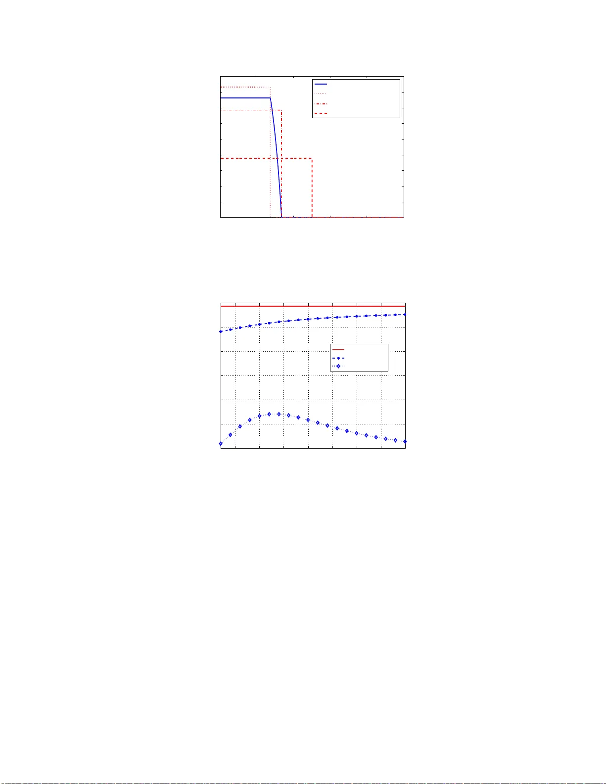
Capacity Deﬁnitions for General Channels with Recei v er Side Information Michelle Ef fros, Senior Member , IEEE, Andrea Goldsm ith, F ellow , IEEE, and Y ifan Liang, Student Member , IEEE Abstract W e consider thre e capacity deﬁnition s for general channe ls with channel side info rmation at the receiver , where th e channel is mod eled as a sequence of ﬁnite dimension al cond itional d istributions not ne cessarily stationar y , ergodic, or in formatio n stable. The S hanno n capa city is the highest rate asymptotically ac hiev able with arbitrarily sm all error probab ility . The ca pacity v ersus outage is the highest rate asymptotica lly achiev able with a given prob ability of d ecoder-recogn ized outag e. Th e expected capacity is the h ighest average rate a symptotically achievable with a single enco der and multiple d ecoder s, where the ch annel side inform ation determines the decod er in use. As a spe cial case of channel code s fo r expe cted rate, the co de fo r c apacity versus outage h as two decod ers: one operates in the non-o utage s tates and decod es all transmitted infor mation, and the other o perates in th e outage s tates and decodes nothin g. Expected capacity equals Shann on capacity for channels governed by a stationar y ergodic ran dom p rocess but is ty pically greater for gen eral chan nels. These alternative capacity d eﬁnitions essentially relax the co nstraint tha t all transmitted informatio n mu st be decode d at the r eceiver . W e derive capacity theo rems fo r these capacity d eﬁnitions th rough in formatio n density . Numerical examples are provided to demon strate their connections and differences. W e also discuss the implication of these a lternative capacity deﬁnitions fo r end-to-end d istortion, source-chann el coding and separation. This work was supported by the D ARP A ITMANET program under grant number 1105741-1-TFIND. The material in this paper was presented in part at the IEEE International Symposium on Information Theory , Cambridge, Massachusetts, August 1998 and the IEEE International Symposium on Information Theory , Nice, France, June 2007. M. Effros is wi th the Department of Electrical Engineering, California Instit ute of T echnology , Pasaden a, CA 91125 (email: effro s@caltech.edu). A. Goldsmith and Y . Liang are with the Department of Electrical E ngineering, Stanford Uni versity , Stanford CA 94305 (email: andrea@wsl.stanford.edu; yﬂ@wsl.st anford.edu). October 10, 2018 DRAFT 1 Index T erms Composite channel, Shanno n capac ity , capacity versus outage, o utage capacity , expected c apacity , informa tion den sity , bro adcast strategy , binary sym metric chan nel ( BSC), b inary er asure ch annel ( BEC), source-ch annel coding, sep aration. October 10, 2018 DRAFT 2 Capacity Deﬁnitions for General Channels with Recei v er Side Information I . I N T RO D U C T I O N Channel capacity has a natural operational deﬁniti on : the highest rate at which in formation can b e s ent wit h arbitrarily l ow p robability of error [1, p. 184]. Channel coding t heorems, a fundamental su bject of Shannon t heory , focus on ﬁndin g i nformatio n th eor etical deﬁnit ions of channel capacity , i.e. expressions for channel capacity in terms of the probabilisti c description of various channel mo dels. In his landmark paper [2], Shannon showed the capacity form ula C = max X I ( X ; Y ) (1) for memoryless channels . The capacity formula (1) is further extended to the well-kn own limiti ng expression C = lim n →∞ sup X n 1 n I ( X n ; Y n ) (2) for channels with memory . Dobrushin proved the capacity formula (2) for the c lass of information stable channels i n [3]. Howe ver , t here are channels t hat do not satisfy t he information s table condition and for wh ich t he capacity formula (2) fails to hold. Examples of information u nstable channels inclu de the stationary regular decompos able channels [4], the stat ionary non anticipatory channels [5] and the a ve raged memoryless channels [6]. In [7] V erd ´ u and Han deriv ed the ca pacity C = sup X I ( X ; Y ) (3) for general channels, where I ( X ; Y ) is the liminf in probability of t he normalized information density . The completely general formula (3) does not require any assump tion such as memory- lessness, in formation stabilit y , stationarity , causalit y , etc. The focus of this paper is on one class of such information unst able channels, the composite channel [8]. A composite channel is a collection of channels { W s : s ∈ S } parameterized by s , where each component channel is stati onary and ergodic. The channel realization is determi ned by the random variable S , which is chosen according to some channel state distribution p ( s ) at October 10, 2018 DRAFT 3 the beginning of tra nsmiss ion and then held ﬁx ed. The composite channel model describes many comm unication systems of practical interest, for ins tance, applications wit h s tringent delay con straint su ch t hat a code word m ay no t experience all possible channel states, sy stems with recei ver complexity constraint such that decoding over long bl ocklength is prohibited, and slow fading wireless channels wit h channel coherence ti me l onger than the codeword duration. Ahlswede studied this class of channels under the nam e averag ed channel and obtained a formula for Shannon capacity in [6]. It is also referred to as the mixed channel in [9]. The class of composite channels can be generalized to channels for wh ich the opt imal input distribution induces a joint input-outp ut distribution on which the er godic decomposi tion theorem [10, Theorem 1.8.2] holds, e.g. station ary distributions deﬁned on complete, separable metric s paces (Polish spaces). In thi s case t he channel index s becomes the ergodic mode. Shannon’ s capacity deﬁnition, with a focus on stati onary and ergodic channels, has enabled great i nsight and desi gn in spiration. Howe ver , the deﬁnition is based on asympto tically large delay and i mposes t he const raint t hat all transm itted inform ation be correctly decoded. In the case of compos ite chann els the capacity is dominated by the performance of the “worst” component channel, no matter how small its probabil ity . This high lights t he pessim istic nature of th e Shannon capacity deﬁnition, wh ich forces the use of a si ngle code with arbitrarily small error probabi lity . In g eneralizing th e channel model to deal with s uch scenarios as the composite channel above, we relax the constraints and generalize the capacity deﬁnitions. These new deﬁnition s are fundamental, and they address practical design strategies t hat give better performance than traditional capacity deﬁnitions. Throughout th is paper we assume t he channel state information is revealed to the receiv er (CSIR), but no channel state information is av ailable at th e transmitt er (CSIT). The downlink satellite communi cation system giv es an example where the transmi tter may not have access t o CSIT : the terrestrial receiv ers implement channel estimati on but do not hav e sufﬁcient transmit power to feed back the channel knowledge to the satellite t ransmitter . In other cases, the transmitter may opt for simpli ﬁed strategies which do not impl ement any adaptive transmis sion based on channel st ate, and therefore CSIT b ecomes i rrele vant. The ﬁrst alternative deﬁnition we consider is capaci ty versus outage [11]. In the absence of CSIT , t he t ransmitter is forced to us e a sin gle cod e, but the decoder may d ecide whether th e information can be reliably d ecoded based on CSIR. W e therefore design a codi ng scheme that October 10, 2018 DRAFT 4 works well most o f th e ti me, but wi th som e m aximal probabilit y q , the decoder sees a bad channel and d eclares an outage; in this case, the t ransmitted information is l ost. The encodi ng scheme is design ed to maximize t he capacity for non-outage s tates. Capacity versus outage was pre viously examined in [11] for s ingle-antenna cellular sys tems, and later became a common criterion used in multip le-antenna wireless f ading channels [12]–[14]. In thi s work we formalize the operational deﬁnition of capacity versus ou tage and also give the i nformation-theoretical deﬁnition throu gh the di stribution of the n ormalized informati on density . Another m ethod for dealing with channels of variable quality is to all ow t he recei ver to decode partial transmitted information. Thi s idea can be illust rated us ing the broadcast strategy suggested by Cover [15]. The transm itter views the com posite channel as a b roadcast channel with a col lection of virtual receivers index ed by channel realization S . The encoder u ses a broadcast code and encodes information as if it were broadcasting to th e virtu al receiver s. The recei ver chooses t he appropriate decoder for the broadcast code based on t he channel W S in action. The goal is t o identi fy th e point in the broadcast rate region that maximizes the expected rate , where the expectation i s taken wi th respect t o the state dist ribution p ( S ) on S . Shamai et al. ﬁrst deriv ed the expected capacity for Gaussian sl owly fading channels in [1 6] and later extended the result to MIMO fading channels in [17]. The formal deﬁniti on of expected capacity was introd uced in [8], wh ere upper and lower bounds were also derived for t he expected capacity of any composite channel. Details of the proofs together with a numerical e xample of a c omposi te binary symm etric channel (BSC) appeared recently in [18 ]. Appl ication of the broadcast strategy to mini mize the end-to -end expected dist ortion is also considered i n [19], [20]. The alternative capacity deﬁniti ons are of particular interest for applications where it is desirable to maxi mize av erage recei ved rate even if i t means th at part of th e t ransmitted in- formation is lost and t he encod er does not kn ow the exact delivered rate. In this case t he recei ver either to lerates the information loss or has a m echanism to recove r th e lost informati on. Examples includ e scenarios wit h some acceptable outage probability , communication systems using mul tiresolution or mult iple description source codes such th at partial receive d in formation leads to a coarse but still useful source reconstruction at a l ar ger dist ortion lev el, feedback channels where t he receiv er tells t he transmit ter which symbol s t o resend, or applications where lost source symbols are well approximated by surrounding samples. The recei ved rate a veraged over m ultiple transmissions is a meaningful metric when there are two time horizons in volved: October 10, 2018 DRAFT 5 a s hort time horizon at the end of whi ch decoding has to be performed because o f string ent delay constraint or decoder compl exity cons traint, and a long tim e horizon at the end o f which the overall throughput is e valuated. For example, consi der a wi reless LA N service subscriber . Whene ver the u ser requests a voice or data transm ission over the network, he us ually expects the information to be delivered wit hin a couple of minu tes, i.e. the sho rt time horizon. Howe v er , the servi ce charge is typically calculated on a monthly basis depending on the total or a verage throughput with in the enti re period, i.e. the long t ime horizon. It is worth poin ting ou t that our capacity analysis d oes not apply to the compound channel [21]–[23]. A comp ound channel includ es a collection of channels but does not assume any associated state distri bution and t herefore has no inform ation density distribution, on which the capacity deﬁnition reli es. Our channel model also e xcludes the arbitrarily varyin g channel [21], [24], where the channel st ate changes on each transmi ssion i n a manner that depends on the channel input in o rder to minimize the capacity of the chosen encodin g and decoding strategies. The remaind er of this paper is structured as fol lows. In Section II w e re view h ow the information theoretical deﬁnitions of channel capacity e v olved with channel models, and giv e a fe w deﬁnitions that serve as the b asis for the deve lopment of generalized capacity deﬁnitions. The Shannon capacity is con sidered in Section III, where we provide an alt ernativ e proof of achie vability based on a modi ﬁed notion of typical sets . W e also s how that the Shanno n capacity only depends o n t he support set o f the channel s tate di stribution. In Section IV we give a formal deﬁnition of t he capacity versus outage and compare it with the closely-related concept of ǫ - capacity [7]. In Section V we introduce the expected capacity and establish a b ijection between the expected-ra te code and the broadcast channel code. In Section VI we com pare capacity deﬁnitions and their i mplications t hrough two examples: t he Gi lbert-Elliott channel and the BSC with random crossover probabil ities. Th e implication of these alternative capacity deﬁnition s for end-to-end d istortion, source-channel coding and separation is brieﬂy discussed in Section VII. Conclusions are giv en in Section VIII. I I . B AC K G RO U N D Shannon in [2] deﬁned the channel capacity as t he supremum of all achiev able rates R for which there exists a sequence of (2 nR , n ) codes such that the probabi lity of error tends to zero October 10, 2018 DRAFT 6 as the blocklength n approaches in ﬁnity , and showed the capacity formul a (1) C = max X I ( X ; Y ) for memoryless channels. In p roving the capacity formula (1), the con verse of the codin g theorem [1, p. 206] u ses Fano’ s inequality and establi shes t he right-hand side of (1) as an upper bound of the rate o f any sequence of channel codes with error probability approaching zero. The direct part of the codin g theorem then shows any rate below the capac ity i s indeed achiev able. Although the capacity formul a (1) is a s ingle-letter expression, the direct channel coding theorem requires coding over long blocklength to achieve arbitrarily small error probabili ty . The receive r decodes by joint typicality with the ty pical set deﬁned as [1, pp. 195] A ( n ) ǫ = n ( x n , y n ) ∈ X n × Y n :     − 1 n log p ( x n ) − H ( X )     < ǫ,     − 1 n log p ( y n ) − H ( Y )     < ǫ,     − 1 n log p ( x n , y n ) − H ( X, Y )     < ǫ  , (4) which relies on th e law of l ar ge numbers to obtain the asym ptotic equiparti tion property (AEP). For channels wit h memory , the capacity formul a (1) generalizes to the li miting expression (2) C = lim n →∞ sup X n 1 n I ( X n ; Y n ) . Howe v er , the capacity formula (2) does not hold in ful l g enerality . Dob rushin proved it for the class of informati on stable chann els. The class of i nformation stabl e chann els, inclu ding the class of memoryless channels as a special case, can be roughly described as having the property th at the input maximi zing the mutual informatio n I ( X n ; Y n ) and its correspond ing output behav e er godically . In a sens e, an ergodic s equence is th e most general dependent sequence for which the strong law of large num bers holds [1, p. 474]. The codi ng theorem of inform ation stable channels follows simil arly from that of mem oryless channels. Howe v er , the joint typicalit y decoding technique cannot be generalized to information u nstable channels. For general channels, the set A ( n ) ǫ deﬁned in (4) does no t ha ve the AEP . As an evidence, the probabili ty of A ( n ) ǫ does not approach 1 for large n . W e may no t construct channel codes which has small error p robability and meanwhi le h as a rate arbitrarily close to (2). Therefore, the October 10, 2018 DRAFT 7 right-hand side of (2), although sti ll a v alid upper bound of channel capacity , is not necessarily tight. In [7] V erd ´ u and Han presented a tight upper bound for general channels and showed its achie vability through Feinstein’ s lemma [25]. W e provide an alternative proof of achieva bility based on a new notion of typical set s in Section III. This informatio n stable conditio n can be i llustrated usin g the concept of informati on density . Deﬁnition 1 (Inf ormation Density) Give n a joint distribution P X n Y n on X n × Y n with marginal distributions P X n and P Y n , the information density i s d eﬁned as [26] i X n Y n ( x n ; y n ) = log P X n Y n ( x n , y n ) P X n ( x n ) P Y n ( y n ) = log P Y n | X n ( y n | x n ) P Y n ( y n ) . (5) The distri bution of the random variable (1 / n ) i X n Y n ( x n ; y n ) is refe rred t o as t he infor mation spectrum of P X n Y n . It is obs erved that the normalized mutual in formation 1 n I ( X n ; Y n ) = X ( x n ,y n ) p ( x n , y n ) · 1 n log p ( y n | x n ) p ( y n ) is the expectation of the normalized inform ation density 1 n i ( x n ; y n ) = 1 n log p ( y n | x n ) p ( y n ) with respect to the underlying j oint input-out put distribution p ( x n , y n ) , i. e. 1 n I ( X n ; Y n ) = E X n Y n  1 n i X n Y n ( X n ; Y n )  . Denote by X n ∗ the input distribution that maximizes the mutual informati on I ( X n ; Y n ) and by Y n ∗ the corresponding outp ut distribution. The i nformation stable conditio n [27, Deﬁnition 3] requires that the normalized information density (1 /n ) i ( X n ∗ ; Y n ∗ ) , as a random v ariable, con verges in distribution to a constant equal to the normalized mutual information (1 /n ) I ( X n ∗ ; Y n ∗ ) as the blocklength n approaches inﬁnity . In [7] V erd ´ u and Han derived the capacity formula (3) C = sup X I ( X ; Y ) for general channels, where I ( X ; Y ) is the liminf in probability of t he normalized information density . In contrast to information stable channels where the distribution of (1 /n ) i ( X n ; Y n ) con ve rges to a s ingle point, for inform ation unstable channels, ev en w ith inﬁnite b locklength the October 10, 2018 DRAFT 8 support set 1 of th e distribution of (1 /n ) i ( X n ; Y n ) may still have multipl e points or e ven contain an int erv al. The Shannon capacity equals the inﬁmum of this suppo rt set. The information spectrum of an information stable channel is demonstrated in the upper plot of Fig. 1. As the block l ength n increases, the con ver gence of the normalized i nformation densi ty to the channel capacity fol lows from the weak law of large numbers. In the lower plot of Fig. 1, we show th e emp irical distribution o f (1 /n ) i ( X n ; Y n ) for an information unstable chann el. The distribution of t he norm alized informati on density does not con v erge t o a singl e point, so t he equation (2) does not equal the capacity , whi ch is giv en by (3). P S f r a g r e p l a c e m e n t s p  1 n i ( x n ; y n )  p  1 n i ( x n ; y n )  I ( X ; Y ) 1 n i ( x n ; y n ) 1 n i ( x n ; y n ) lim n →∞ 1 n I ( X n ; Y n ) lim n →∞ 1 n I ( X n ; Y n ) n = 1 n = 1 n = 10 n = 10 n = 100 0 n = ∞ n = ∞ Fig. 1. Empirical distribution of normalized information density . Upper: information stable channel. Lower: information unstable channel. I I I . S H A N N O N C A PAC I T Y W e consider a channel W which is s tatistically m odeled as a sequence of n -dimensi onal conditional distributions W = { W n = P Z n | X n } ∞ n =1 . For any integer n > 0 , W n is the con ditional distribution from the input space X n to the output space Z n . Let X and Z denot e the i nput and output processes, respectively , for the given sequence of channels. Each process is speciﬁed by a sequence of ﬁnite-dim ensional distributions, e.g. X = { X n = ( X ( n ) 1 , · · · , X ( n ) n ) } ∞ n =1 . 1 The smallest closed set of which t he complement set has probability measure zero. October 10, 2018 DRAFT 9 T o consi der the special case where the decoder has recei ver sid e information not present at the encoder , we represent th is side information as an additional output of the channel. Speciﬁcally , we let Z n = ( S, Y n ) , where S is the channel s ide information and Y n is the o utput of the channel described by parameter S . Throughout, we assume t hat S is a random variable ind ependent of X and unknown to the encoder . Thus for each n P W n ( z n | x n ) = P Z n | X n ( s, y n | x n ) = P S ( s ) P Y n | X n ,S ( y n | x n , s ) , and th e information density (5) can be rewritten as i X n W n ( x n ; z n ) = log P W n ( z n | x n ) P Z n ( z n ) = log P Y n | X n ,S ( y n | x n , s ) P Y n | S ( y n | s ) = i X n W n ( x n ; y n | s ) . (6) In the following we see that th e generalized capacity deﬁnitions of compo site channels d epend crucially on information density inst ead of mut ual inform ation. W e also denote by F X ( α ) the limit of the cum ulative distribution function (cdf) of the normalized in formation density , i.e. F X ( α ) = lim n →∞ P X n W n  1 n i X n W n ( X n ; Y n | S ) ≤ α  , (7) where the subscript emphasizes the inpu t process X . Consider a sequence of (2 nR , n ) cod es for channel W , where for any R > 0 , a (2 nR , n ) cod e is a col lection o f 2 nR blocklength- n chann el cod e words and th e associated decoding regions. The Shannon capacity i s deﬁned as the sup remum of all rates R for which there exists a sequence of (2 nR , n ) codes with v anishing error probabil ity [2]. Therefore, the Shannon capacity C ( W ) measures the rate that can be reliably transmitted from the encoder and als o be reliably received at th e decoder . W e simpli fy this notati on to C if the channel ar gument is clear from context. The achiev ability and conv erse theorems for the Shannon capacity of a general channel C = sup X I ( X ; Z ) = sup X I ( X ; Y | S ) = sup X sup { α : F X ( α ) = 0 } ( 8) are proved, respectiv ely , by Theorems 2 and 5 of [7], using Feinstein’ s lemma [25], [9, Lemma 3.4.1], [28, Lemm a 3.5.2] and the V erd ´ u-Han lemma [7, Th eorem 4]. The special case of a comp osite channel with CSIR follows imm ediately from th is result. W e here p rovide an October 10, 2018 DRAFT 10 alternativ e proo f of achiev ability based on a m odiﬁed notion of typi cal sets . In the following proof we simpli fy notations by removing the explicit conditi oning on th e side information S . Encoding : For any input distribution P X n , ǫ > 0 , and R 0 , the typical set A ( n ) ǫ is deﬁned as A ( n ) ǫ =  ( x n , y n ) : 1 n i X n W n ( x n ; y n ) ≥ I ( X ; Y ) − ǫ  . (9) Channel ou tput Y n is decoded to X n ( i ) where i is the u nique ind ex for which ( X n ( i ) , Y n ) ∈ A ( n ) ǫ . An error is declared if more t han one or no such index exists. Err or Analysis : W e deﬁne the following e vents for all indices 1 ≤ i, j ≤ 2 nR , E j i =  ( X n ( j ) , Y n ) ∈ A ( n ) ǫ   X n ( i ) sent  . (10) Conditioned on code word X n ( i ) being sent, the probabili ty of the corresponding error e vent E i E i = [ j 6 = i E j i [ E c ii , can be bounded by Pr( E i ) ≤ Pr( E c ii ) + X j 6 = i Pr( E j i ) . Since we generate i.i. d. codew ords, Pr( E ii ) and Pr( E j i ) , j 6 = i , do not depend on the speciﬁc indices i , j . Assuming equiprobabl e inputs , the e xpected probability of error wi th respect to the randomly generated codebook is: P ( n ) e = Pr { error | X n (1) sent } ≤ Pr( E c 11 ) + 2 nR X j =2 Pr( E j 1 ) ≤ P X n W n  1 n i X n W n ( X n (1); Y n ) < I ( X ; Y ) − ǫ  + 2 nR X ( x n ,y n ) ∈ A ( n ) ǫ P X n ( x n ) P Y n ( y n ) ≤ ǫ n + 2 n [ R − I ( X ; Y )+ ǫ ] X ( x n ,y n ) ∈ A ( n ) ǫ P X n W n ( x n , y n ) , (11) October 10, 2018 DRAFT 11 where by deﬁnition o f I ( X ; Y ) we hav e ǫ n approaching 0 for n large enough. The last inequality uses (6), (9), and the fact that ( x n , y n ) ∈ A ( n ) ǫ implies 1 n i X n W n ( x n ; y n ) = 1 n log P X n W n ( x n , y n ) P X n ( x n ) P Y n ( y n ) ≥ I ( X ; Y ) − ǫ and consequ ently P X n ( x n ) P Y n ( y n ) ≤ 2 − n [ I ( X ; Y ) − ǫ ] P X n W n ( x n , y n ) . From (11) P ( n ) e ≤ ǫ n + 2 n [ R − I ( X ; Y )+ ǫ ] → 0 for all R 0 , which completes our proof. Although a comp osite channel is characterized by the collection of component channels { W s : s ∈ S } and the associated probability distribution p ( s ) on S , the Shannon capacity of a composite channel is solely determined by the support set of the channel state distribution p ( s ) . In the case of a discrete channel state set S , we only need to kno w which channel states have po sitive probability . The exact positive v alue th at the probabi lity mass function p ( s ) assigns to channel states is irrele vant in v iew of the Shannon capacity . In the case of a continuous channel state set S , we only need to kno w the subset of channel states where the probabi lity density function is strictly positive . This is formalized in Lemma 1 . Before introducing t he lemma w e need t he following deﬁnition [29, Appendi x 8]. Deﬁnition 2 (Equi valent Prob ability Measure) A probability measure p 1 is absolutely contin- uous with r espect t o p 2 , writ ten as p 1 ≪ p 2 , if p 1 ( A ) = 0 i mplies th at p 2 ( A ) = 0 for any eve nt A . Here p i ( A ) , i = 1 , 2 , is th e probabi lity of event A und er probability m easure p i . p 1 and p 2 are equi valent pr obability measur es if p 1 ≪ p 2 and p 2 ≪ p 1 . Lemma 1 Consider two comp osite channels W 1 and W 2 with component channels from the same collection { W s : s ∈ S } . Denote by p 1 ( s ) and p 2 ( s ) , respectiv ely , the corresponding channel state distribution of each composit e channel. Then p 1 ≪ p 2 implies C ( W 1 ) ≤ C ( W 2 ) . Furthermore, if p 1 and p 2 are equiv alent probability measures, then C ( W 1 ) = C ( W 2 ) . Intuitively speaking, p 1 ≪ p 2 if th e support set for W 2 is a subset of the support set for W 1 , so any input di stribution that allows reliable t ransmission on W 1 also allows reliable transmiss ion on W 2 . p 1 and p 2 are equiv alent probability measures if they sh are the same suppo rt set, and this October 10, 2018 DRAFT 12 guarantees that the corresponding composite channels ha ve the sam e Shannon capacity . Details of the proof are given in Appendix A. The equ iv alent probability m easure is a sufﬁcient but not necessary condit ion for two com pos- ite channels to have the same Shannon capacity . For e xample, consid er two slow-fading Gaussian composite chann els. It is possible that two probability m easures have no support below t he sam e channel gain , but one assigns non-zero probability to states with large capacity while the other does not. In th is case, the probabili ty m easures are not equiva lent; nevertheless the Shannon capacity of both com posite channels are the same. I V . C A P A C I T Y V E R S U S O U T AG E The Shannon capacity deﬁnition i mposes the constraint that all transm itted information be correctly decoded at t he receiv er wi th vanishing error p robability , while in some real system s it i s acceptable to lose a sm all portion o f the transmit ted information as long as there is a mechanism to cope with the packet loss. For example, in s ystems with a receiver complexity constraint , decoding over ﬁnite blocklengt h i s necessary but in th e case of packet loss, ARQ (automat ic repeat request) protocols are im plemented where the recei ve r requests retransmission of the lost information [30], [31]. If the sy stem has a strin gent delay constraint, lost informatio n can be approximated from the c ontext, for example the block-coded JPEG image transmissio n over noisy channels where missin g blocks can b e reconstructed in th e frequency domain by in terpolating the discrete cosine transformati on (DCT) coefﬁ cients of av ailable neighboring bl ocks [32]. These examples demon strate a new noti on o f capacity versus out age : the transmitter sends information at a ﬁxed rate, which is correctly receiv ed m ost of the time; with some maximal probability q , the decoder sees a bad channel and declares an outage, and the trans mitted informatio n is l ost. This is formalized in the fol lowing deﬁnition: Deﬁnition 3 (Capacity versus Outage) Cons ider a composite channel W with CSI R. A (2 nR , n ) channel code for W consists of the following: • an encodi ng function X n : U = { 1 , 2 , · · · , 2 nR } → X n , where U is the message index set and X is the inp ut alphabet; • an outage id entiﬁcation function I : S → { 0 , 1 } , where S is the set of channel states; • a decoding fun ction g n : Y n × S → ˆ U = { 1 , 2 , · · · , 2 nR } , which only operates when I = 1 . October 10, 2018 DRAFT 13 Deﬁne the outage p robability P ( n ) o = Pr { I = 0 } and th e error probability in no n-outage states P ( n ) e = Pr { U 6 = ˆ U | I = 1 } . A rate R i s outage- q achiev able if there exists a sequence of (2 nR , n ) channel codes such that lim n →∞ P ( n ) o ≤ q and lim n →∞ P ( n ) e = 0 . Th e capacity versus outage C q of the channel W with CSIR is deﬁned to be the supremu m over all outage- q achiev able rates. In the above deﬁnition, P ( n ) o is the prob ability that t he decoder , using its side information about the channel, determ ines i t cannot reliably decode t he recei ved channel output and declares an o utage. In contrast, P ( n ) e is the probability that the receive r decodes improperly gi ven that an outage is not declared. Deﬁnition 3 can be viewed as an operational deﬁnition of the capacity versus outage. In parallel to the dev elopment of the Shannon capacity , we also gi ve an information theor etic deﬁnition [1, p. 18 4] of the capacity versus outage C q = sup X I q ( X ; Y | S ) = sup X sup { α : F X ( α ) ≤ q } . (12) Notice t hat C 0 = C , so the capacity versus outage is a generalization of the Shannon capacity . The achie vability p roof foll ows th e same ty pical-set argument giv en in Section III. The con verse result likewise follows [7]. Details are giv en in App endix B. The concept of capacity versus outage was initially proposed in [11 ] for cellul ar m obile radios. See also [33, Ch. 4] and references therein for more details. A closely -related concept of ǫ -capacity was deﬁned in [7]. Howe ver , there is a subtle difference between the two: in the deﬁnition of ǫ -capacity the non-zero error probabil ity ǫ accounts for decoding errors undetected at the receiver . In contrast, in the deﬁnition of capacity versus outage the receiv er declares an outage when the channel state do es not allow the receive r to decode with vanishing error probability . Asym ptotically , the probability o f error must be bounded by so me ﬁxed constant q and all errors must be r ec ognized at t he decoder . As a consequence, no decoding is performed for outage states. If the power consumption to perform receiver decoding becom es an issue, as in the case of sens or n etworks wit h non-rechar geable nodes or power -conserving m obile devices, October 10, 2018 DRAFT 14 then we should disting uish between decoding with error and no decoding at all in view of ener gy conservation. This sub tle difference also has important consequ ences when we con sider end -to-end com mu- nication performance using source and channel codi ng. When the outage s tates are recognized by the recei ver , i t can request a retransm ission or simply reconstruct the source symbo l by its mean – giving an expected distortion equal to the source variance. In contrast , if the recei ver cannot recognize the decoding error as i n the case of an ǫ -capacity channel code, the reconst ruction based on t he incorrectly decoded sym bol m ay lead to not only lar ge distortion but also loss o f synchronization in the source code’ s decoder . W e can further deﬁne t he outage capacity C o q = (1 − q ) C q as the long-term a verage rate, if the channel is used repeatedly and at each use the channel state is drawn independent ly according to p ( s ) . The transmit ter u ses a si ngle codebook and sends information at rate C q ; the recei ver can correctly decode the information a proportion (1 − q ) of the time and turns itself off a proporti on q o f the tim e. T he out age capacity C o q is a m eaningful metric if we are onl y interested in the fraction of correctly recei ved packets and approx imate the unreliable packets by surroundin g samples. In this case, optimizi ng ov er the ou tage probabilit y q to maxim ize C o q guarantees performance that is at least as good as the Shannon capacity and may be far better . As another example, if all informatio n m ust be correctly decoded eventually , th e packets that suf fer an outage have t o be retransmitted. Th is dem ands so me repetiti on mechanism t hat is usually implemented in the link-layer error control of dat a communi cation. The number of channel uses K to transmit a packet of size ( N = C q ) bi ts has a geometric distribution Pr { K = k } = q k − 1 (1 − q ) , and the expected value is 1 (1 − q ) = N C o q , which also ill ustrates C o q as a measure of t he long-term a verage throughput . Next we brieﬂy analyze t he capacity versus outage from a computational p erspectiv e. W e need the fol lowing deﬁnition before we proceed: Deﬁnition 4 (Pr obability- q Compatible Subchann el) Consider a comp osite channel W with state distribution p ( s ) , s ∈ S . Consider another channel W q where the channel state set S q is a subset of S ( S q ⊆ S ). W q is a pr obability- q compatibl e subchannel of W i f Pr {S q } ≥ 1 − q . October 10, 2018 DRAFT 15 Note that W q is not exac tly a composite channel since we only specify the state set S q but not the correspond ing state di stribution over S q . Howe ver , we will only be interested in the Shannon capacity of W q , and as po inted out by Lemma 1, th e exact distribution ov er S q is irrele vant t o determine this capacity . The capacity versus o utage as deﬁned i n (12) requi res a two-stage optimi zation. In the ﬁrst step we ﬁx th e inp ut distribution X and ﬁnd the probabilit y- q com patible sub channel th at yi elds the highest achie vable rate. In the s econd step we optim ize over the dis tribution of X . This view is more conv enient if the opti mal input distri bution can be easily determi ned. W e then ev aluate the achiev able rate of each compon ent channel wi th this optim al input and declare ou tage for those with the l owest rates. As an example, cons ider a s low-f ading MIMO channel with m transmit antennas. As sume the channel matrix H has i .i.d. Rayleig h fading coefﬁcients. The outage probabili ty associated with transmit rate R is k nown to be [34] P o ( R ) = inf Q  0 , Tr ( Q ) ≤ m Pr  log det  I + SNR m H Q H †  ≤ R  , and the capacity versus outage is C q = sup { R : P o ( R ) ≤ q } . Although the optimal input cov ariance m atrix Q is u nknown i n general, it i s shown in [14] that there is no loss of generality in assuming Q = I in the high SNR regime and th e corresponding capacity versus outage simpliﬁes to C q = sup  R : Pr  log det  I + SNR m H H †  ≤ R  ≤ q  . By reversing the order o f t he two optimi zation steps we have another i nterpretation of capacity versus outage C q = sup W q C ( W q ) . (13) Here we ﬁrst determine the Shannon capacity of each prob ability- q compatible subchannel, then optim ize by choosing the one with the highest Shannon capacity . Thi s view h ighlights the connection between C q of a composite chann el and the Shannon capac ity of its probability- q compatible su bchannels, and i s more conv enient if th ere is an intrins ic “ordering” of the component channels. For e xample cons ider a de graded collection of channels w here for any channel st ates s 1 and s 2 there exists a transition prob ability p ( y n 2 | y n 1 ) su ch that p ( y n 2 | x n , s 2 ) = X y n 1 p ( y n 1 | x n , s 1 ) p ( y n 2 | y n 1 ) . October 10, 2018 DRAFT 16 The degraded relati onship can be extended to the less noisy and more capable conditions [35]. The m ore capable condition requires 2 I ( X n ; Y n 1 | s 1 ) ≥ I ( X n ; Y n 2 | s 2 ) (14) for any input distribution X . It is the weakest of all three b ut sufﬁces to establi sh an ordering. The opt imal probabilit y- q comp atible subchannel W ∗ q has th e smallest set of channel states S ∗ q such that any component channel within S ∗ q is more capable t han a component channel not i n S ∗ q . Th e Shannon capacity of W ∗ q equals the capacity versus out age- q of the orig inal channel W . V . E X P E C T E D C A PAC I T Y The deﬁnition of capacity versus out age in Section IV is essentially an all-or-nothing g ame: the recei ver may declare outage for u ndesirable channel st ates but is otherwise required to decode all transmitted informati on. There are examples where partia l received inform ation is useful. Consider sending a mult i-resolution source code over a composite channel. Decoding all t ransmitted information l eads to reconstruction wi th the lowest dist ortion. Howe ver , in the case of inferior channel quality , it still helps to decode partial information and get a coarse reconstruction. Al though t he transm itter sends i nformation at a ﬁxed rate, the notion of expected capacity allows the recei ver to decide in expectation how much in formation can be correctly decoded based on channel realizations. Next we i ntroduce some not ation which is useful for the formal deﬁnition of the expected capacity . Con v entionally we represent in formation as a message ind ex, c.f. the Shannon capacity deﬁnition [1, p. 193] and the capacity versus outage deﬁnition in Section IV. T o deal with partial information, here we represent information as a bl ock of bits ( b i ) i ∈I , where I i s the set of bit indices. Denote by M ( I ) = { ( b i ) i ∈I : b i binary } the set o f all pos sible blocks o f information bi ts with bi t i ndices from the set I . Each element in M ( I ) is a bit -vector of length |I | , so the size of the set M ( I ) is 2 |I | . If another index set e I is a proper subset of I ( e I ⊂ I ), then M ( e I ) represents some partial information with respect 2 Assuming each component channel i s stationary and ergodic, the mutual information in (14) is well deﬁned. October 10, 2018 DRAFT 17 to th e full information M ( I ) . This representation generalizes the con ventional representation using m essage indices. Deﬁnition 5 (Expected Capacity) Consider a composite channel W with channel state distri- bution p ( s ) . A (2 nR t , { 2 nR s } , n ) code consists of the fol lowing: • an encoding fun ction f n : M ( I n,t ) = { ( b i ) i ∈I n,t } → X n , where I n,t = { 1 , 2 , · · · , nR t } is the index set of t he transm itted in formation bi ts and X is the input alphabet; • a collection of decoders, one for each channel s tate s , g n,s : Y n × S → M ( I n,s ) = { ( ˆ b i ) i ∈I n,s } where I n,s ⊆ I n,t is the set of indices of the decodable information bits in channel state s . |I n,s | = nR s . Deﬁne the decoding error probabilit y associated with channel state s as P ( n,s ) e = Pr n ∪ i ∈I n,s ( ˆ b i 6 = b i ) o , and th e av erage error probability P ( n ) e = E S P ( n,S ) e = Z P ( n,s ) e p ( s ) ds. A ra te R = E S R S is achiev able in expectation if there exists a sequence of (2 nR t , { 2 nR s } , n ) codes with avera ge error prob ability lim n →∞ P ( n ) e = 0 . T he expected capacity C e ( W ) is the supremum of all rates R achiev able in expectation. W e want to emphasize a few subt le po ints in the above deﬁnition. In chann el state s the receiv er only d ecodes those information bits ( b i ) with indices i ∈ I n,s . Decoding error occurs if any of th e decoded in formation bi ts ( ˆ b i ) is different from the transmitted information bit ( b i ) . No attempt i s made to decode i nformation bits with indices o ut of the i ndex set I n,s ; hence these information bits are i rrele vant to the error analysis for channel st ate s . The cardinality nR s of the index set I n,s depends only on the blocklength n and th e channel state s . Among the transmitted nR t information bits , the transm itter and th e receive r can agree on t he set of decodable information b its for each channel state before transmissio n starts, i.e. not October 10, 2018 DRAFT 18 only the cardinalit y of I n,s , b ut the set I n,s itself is un iquely determined by the channel state s . Ne vertheless, for the same channel state s , the recei ver may choose to decode dif ferent sets o f information bits depending on the actual channel output Y n , alt hough all these sets are of t he same cardinality nR s . In this case t he set of decodabl e information bits for each channel state is unknown to t he transmitt er beforehand. W e ﬁrst look at the case where the transmitter and the receive r agree on t he set o f decodable information bit s for each channel st ate. In a composite channel the transmitter can vie w t he channel as a broadcast channel wi th a coll ection of v irtual receive rs indexed by channel real- ization S . The encoder uses a broadcast code t o transmit to the virtu al receiv ers. Th e receiv er uses the side information S to choose the appropriate decoder . Before we proceed to establ ish a connection b etween the expected capacity of a compos ite channel and the capacity region of a broadcast channel, we state the following deﬁnition o f th e broadcast capacity region, which is a direct extension from t he two-user case [1, p. 421] to the mu lti-user case. Consider a broadcast chann el with m recei vers. The receiv ers are ind ex ed b y the s et S with cardinality m , which is remini scent of the index set of channel st ates in a composit e channel. The power set P ( S ) (or simply P ) i s the set of all subs ets o f S . The cardinality of the power set i s |P ( S ) | = 2 m . Deﬁnition 6 (Br oadcast Channel Capacity Region) A ( { 2 nR p } , n ) code for a broadcast chan- nel cons ists of the following: • an encoder f n : Y p ∈P , p 6 = φ M p → X n , where φ is the empty set, p ∈ P ( S ) is a non-empty subset of users, and M p = { 1 , 2 , · · · , 2 nR p } is the message set intended for u sers wi thin the subset p o nly . The short-hand notati on Q p M p denotes the Cartesian product of the corresponding message sets; • a collection of m decoders, one for each user s , g n,s : Y n s → Y p ∈P , s ∈ p ˆ M p , where Y n s is the channel output for user s . October 10, 2018 DRAFT 19 Deﬁne the error event E s for each user as E s =  g n,s ( Y n s ) =  ˆ M p  p ∈P : s ∈ p 6 =  M p  p ∈P : s ∈ p  , (15) and th e overall probability of error as P ( n ) e = Pr ( [ s E s ) . A rate vector { R p } p ∈P is broadcast achiev able if there exists a sequence of ( { 2 nR p } , n ) cod es with lim n →∞ P ( n ) e = 0 . The br oadcast channel capacity r e gion C BC is the con vex closure of all broadcast achiev able rate vectors. In t he above deﬁnit ion, we explicitly distinguis h bet ween priv ate and com mon informati on. The message set M p contains inform ation decodable by all users s ∈ p but no others. For instance, in a three-user BC we ha ve p riv ate information M 1 , M 2 , M 3 , information for any pair of users M 12 , M 23 , M 13 , and the comm on inform ation M 123 . Th e to tal num ber of message sets is 2 m − 1 since the empty set φ is excluded. W e establish a connection between the expected capacity of a composite channel and t he capacity region of a broadcast channel th rough the following theorem. For ease of notation we state the theorem for a ﬁnite number of users (channel states). The result can be generalized to an inﬁnite number of u sers (continuous channel stat e alphabets) using t he standard technique of [36, Ch. 7 ], i.e. to ﬁrst dis cretize the continuous channel state distribution and then take the limitin g case. Theor em 1 Consider a composite channel characterized by the jo int dis tribution P W n ( s, y n | x n ) = P S ( s ) P Y n | X n ,S ( y n | x n , s ) , and th e corresponding BC with the channel for each recei ver satisfying P Y n s | X n ( y n s | x n ) = P Y n | X n ,S ( y n s | x n , s ) . Denote by C e the expected capacity of the comp osite channel and by C BC the capacity region of the corresponding BC, as in Deﬁnitions 5 and 6, respectively . If the set of decodable information bits in the com posite channel is uni quely determined by the channel state S , then the expected capacity sati sﬁes C e = sup ( R p ) ∈C BC X p ∈P R p X s ∈ p P S ( s ) = sup ( R p ) ∈C BC X s ∈S P S ( s ) X s ∈ p R p . (16) October 10, 2018 DRAFT 20 The proof establishes a two-wa y mapping: any ( { 2 nR p } , n ) code for the broadcast channel can be mapped t o a (2 nR t , { 2 nR s } , n ) expected-rate code for t he com posite channel and vice versa, where th e mapping satisﬁes R s = P s ∈ p R p for channel s tate s . The d etails are g iv en in Ap pendix C. Although we hav e introduced a new n otion o f capacity , t he conn ection established in Theorem 1 shows that the tools developed for broadcast codes can be appl ied to deriv e corresponding expected capacity results, with the addition of an optimi zation to choose the point on th e BC rate region boundary that maximizes the expected rate. For example, in [17] s ome subo ptimal approaches, i ncluding s uper-majorization and one-di mensional approxim ation, were introdu ced to analyze the expected capacity of a s ingle-user slowly fading M IMO channel. After the full characterization of the MIMO BC capacity region through the w ork [37]–[41], the expected capacity of a slowly fading MIMO channel can be obtained by choosing the op timal op erating point on the bou ndary of the dirty-paper coding (DPC) region. The connection in Theorem 1 als o shows that any expected-rate code d esigned for a composit e channel can be put into the framework of BC code design . Strategies l ike l ayer ed sour ce coding with pr ogr essive transmis sion , proposed in [42], imm ediately generalize to the broadcast coding problem. Ass uming t here are only two channel states s 1 and s 2 , th is strategy divides the entire transmissio n bl ock into two segments. Th e information transmitted in the ﬁrst segment is intended for both s tates, and that in the second s egment is intended for the better channel state s 2 only . This s trategy can be easily m apped to a BC code with individual i nformation M 2 and common information M 12 , and orthogonal channel access. Furthermore, the complexity of d eriving a single point on the BC region boundary is similar t o that of deri ving the expected capac ity under a speciﬁc channel state distribution. The ent ire BC region bou ndary can be traced out by var ying t he channel state dist ributions. W e want to emp hasize that in Th eorem 1 the conditi on t hat the transmitter knows the set of decodable information bits in advance is not su perﬂuous. If the recei ver chooses to decode diffe rent sets of information bit s depending on the actual channel output Y n , and consequently the t ransmitter does not kn ow the s et of decodable information bit s for each state s , then the mapping b etween expected-rate codes and BC codes may not exist. In the following we give an example where the expected capacity exceeds the supremum of expected rates achiev able by BC codes. Consider a binary erasure channel (BEC) where the erasure probabi lity takes two October 10, 2018 DRAFT 21 equiprobable values 0 ≤ α 1 < α 2 ≤ 1 . In Appendi x D we show th at th e maxi mum expected rate achiev able by BC codes i s R = max  1 − α 2 , 1 − α 1 2  . (17) Howe v er , we can transmit uncoded informatio n bits directly over this composi te BEC. In the limit o f l ar ge blocklength n , th e receiv er can successful ly decode n (1 − α i ) bits for channel states α i , i = 1 , 2 , b y sim ply inspecting the channel out put, although these successfull y decoded information bits cannot be determined at the transmi tter a priori . Overall the expected capacity C e = 1 − α 1 + α 2 2 exceeds the maxim um expected rate achiev able by BC codes. Notice, howev er , these two channel codes are extremely differe nt from an end-to-end coding p erspectiv e. The broadcast strategy may be combined with a multiresoluti on so urce code. In contrast, t he sou rce cod ing strategy required for the uncoded case is a multi ple description source code with single-bit descript ions. D ue to this d iffe rence, it i s not obvious which scenario yields the lower end-to-end distortio n. The comparison depends on the channel state dist ribution and the rate-distortion function of the source. Regardless of the transmitter’ s k nowledge about decodable information b its, we s how that C e satisﬁes the lower bound C e ≥ sup q C o q and th e upper b ound C e ≤ sup X lim sup n →∞ E S E X n Y n | S  1 n i X n W n ( X n ; Y n | S )     S  . (18) The lower bound is achieved using the channel code for capacity versus outage- q , which achieve s a rate C q a proportion (1 − q ) of the time and zero otherwise. F or the upper bound, we assume channel side i nformation is provided to the transmitt er (CSIT) so it can adapt the transm ission rate to the channel state. In this case, the achiev able expected rate can only be imp roved. The proof is giv en in Ap pendix E. V I . E X A M PL E S In this section we con sider s ome examples to illustrate various capacity deﬁnition s. October 10, 2018 DRAFT 22 A. Gilbert -Elliott Channel The Gilbert-Ell iott channel [43] is a two-state Markov chain, where each state is a BSC as shown in Fig. 2. The crossover probabi lities for the “good” and “bad” BSCs sati sfy 0 ≤ p G < p B ≤ 1 / 2 . The transition probabilities between the states are g and b respectiv ely . The initial state distribution is given by π G and π B for states G and B . W e let x n ∈ { 0 , 1 } , y n ∈ { 0 , 1 } , and z n = x n ⊕ y n denote the channel input, out put, and error on the n th transmissio n. W e th en study capac ity deﬁnitions when the channel characteristics of stationarity and ergodicity change with the parameters. G B b g 1-g 1 0 0 1 1- 1- p p p B B B 1-b p G p G p G 1 0 0 1 1- 1- P S f r a g r e p l a c e m e n t s p  1 n i ( x n ; y n )  I ( X ; Y ) 1 n i ( x n ; y n ) lim n → ∞ 1 n I ( X n ; Y n ) n = 1 n = 1 0 n = 1 0 0 0 n = ∞ Fig. 2. Gilbert-Elliott Channel Example 1: Er godic Case, Stat ionary or Non-Stat ionary When π G = g / ( g + b ) and π B = b/ ( g + b ) , the Gilbert-Elliott channel is stati onary and ergodic. In this case t he informatio n dens ity 1 n i X n W n ( X n ; Y n ) con ver ges to a δ -function at th e av erage mutual i nformation, so capacity equals av erage mutual information as u sual. Therefore the Shannon capacity C is equal t o th e expected capacity π G C G + π B C B , where C G = 1 − h ( p G ) , C B = 1 − h ( p B ) and h ( p ) = − p log p − ( 1 − p ) log(1 − p ) i s t he binary entropy function. This is a sin gle-state compos ite channel. Since any transmissi on may experience either a go od or a bad channel condition, the receiv er has no basis for choosing to declare an outage on certain transmissio ns and not on others. Capacity versus outage equals Shannon capacity in this case. If π G 6 = g / ( g + b ) but b and g are nonzero, then the Gilbert-Elliott channel is ergodic b ut not stationary . Howe ver , the dist ribution on the st ates G and B con verges t o a stati onary distribution. Thus t he chann el i s asym ptotically mean stationary , and the deﬁnitions of capacity have the same values as in the stationary case. Example 2: Stationary and Noner godic Case October 10, 2018 DRAFT 23 W e no w set g = b = 0 . So th e initial channel state is chosen according t o probabiliti es { π G , π B } and then remains ﬁxed for all time. The Shannon capacity equals that of the bad channel ( C = C B ) . The capacity versus outage- q C q = C B if the outage probability q < π B and C q = C G otherwise. The loss in curred from lack of side informati on at the encoder is that t he expected capacity is strictly less t han th e av erage of individual capacities π B C B + π G C G and is equal to [15] max 0 ≤ r ≤ 1 / 2 1 − h ( r ∗ p B ) + π G [ h ( r ∗ p G ) − h ( p G )] , (19) where α ∗ β = α ( 1 − β ) + (1 − α ) β . The interpretation here is that the broadcast code achie ves rate 1 − h ( r ∗ p B ) for the bad channel and an additio nal rate h ( r ∗ p G ) − h ( p G ) for the go od channel, so the average rate is t he expected capacity . Using the Lagrangian multi plier method we can o btain r ∗ which m aximizes (19). Namely if we deﬁne k = π G π B , A = 1 − 2 p B 1 − 2 p G , f ( p 1 , p 2 ) = log(1 / p 1 − 1) log(1 / p 2 − 1) then r ∗ = 0 if k ≤ Af ( p B , p G ) ; r ∗ = 1 / 2 if k ≥ A 2 and r ∗ solves f ( r ∗ p G , r ∗ p B ) = A/k otherwise. B. BSC with random cr ossover pr o babiliti es In the n on-er godic case, the Gilbert-El liott Channel is a two-state channel, where each state corresponds to a BSC with a dif ferent crossover probabil ity . W e now generalize that example to allow m ore than two states. W e consider a BSC with random crossover p robability 0 ≤ p ≤ 1 / 2 . At t he beginning of time, p is chosen according to some distribution f ( p ) and then held ﬁxed. W e also use F ( p ) = R p 0 f ( s ) ds to denote the cumu lativ e d istribution fun ction. L ike the n on- er godic Gilbert-Elliott channel, this is a mul ti-state composite channel provided { p : f ( p ) > 0 } has cardinali ty at least two. The Shannon capacity is C = 1 − h ( p ∗ ) where p ∗ = sup { p : f ( p ) > 0 } = inf { p : F ( p ) = 1 } , and th e capacity versus ou tage- q is C q = 1 − h ( p q ) where p q = inf { p : F ( p ) ≥ 1 − q } . W e consider a broadcast approach on this channel to achieve the expected capacity . The recei ver is equi v alent to a continuum of ordered users, each indexed by the BSC crossover probability p and occurring with probability f ( p ) d p . If the set { p : f ( p ) > 0 } i s inﬁnite, th en October 10, 2018 DRAFT 24 the transmi tter sends an inﬁnit e number of l ayers of coded information and each user decodes an incremental rate | dR ( p ) | corresponding t o its o wn layer . Since the BSC broadcast channel is degraded, a user with crossover probability p can also decode layers indexed by lar ger crossover probabilities, therefore we achieve a rate of R ( p ) = − Z 1 / 2 p dR ( p ) (20) for recei ver p . The problem of determining th e expected capacity then boils down t o th e characterization of th e broadcast rate region and the choice of the point on that region that maximizes R p R ( p ) f ( p ) dp . In the discrete case with N users, ass uming 0 ≤ p 1 ≤ · · · ≤ p N ≤ (1 / 2) , t he capacity region is shown to be [44] { R = ( R i ) 1 ≤ i ≤ N : R i = R ( p i ) = h ( r i ∗ p i ) − h ( r i − 1 ∗ p i ) } (21) where 0 = r 0 ≤ r 1 ≤ · · · ≤ r N = 1 / 2 . Since the orig inal broadcast channel is stochasti cally degraded it has the same capacity region as a cascade of N BSC’ s . The capacity region boundary is traced ou t by augmenting ( N − 1) auxiliary channels [44] and varying t he crossover proba- bilities of each. For each i , r i equals the overall crossover probabili ty for auxiliary channels 1 up to i . See Fig. 3 for an illustrati on. The resulting expected capacity is C e = max 0= r 0 ≤···≤ r N =1 / 2 N X i =1 f ( p i ) N X j = i [ h ( r i ∗ p i ) − h ( r i − 1 ∗ p i )] . r Auxiliary channel Degraded BSC BC YN Y2 Y1 X N 2 1 N-1 2 1 p p p r r P S f r a g r e p l a c e m e n t s p  1 n i ( x n ; y n )  I ( X ; Y ) 1 n i ( x n ; y n ) lim n → ∞ 1 n I ( X n ; Y n ) n = 1 n = 1 0 n = 1 0 0 0 n = ∞ Fig. 3. BSC broadcast channel with auxiliary channels for random coding W e extend the a bove result to the continuous case with a n inﬁnite number of auxiliary channels. In this case we deﬁne a m onotonically increasing function r ( p ) equal to the overall crossover October 10, 2018 DRAFT 25 probability of auxil iary channels up to th at indexed by p . In the fol lowing we use r ( p ) and r p interchangeably . For the layer in dexe d by p , the i ncremental rate is − dR ( p ) = h ( p ∗ r p ) − h ( p ∗ r p − dp ) . Using the ﬁrst order approxim ation r p − dp ≈ r p − r ′ p dp and h ( x − δ ) ≈ h ( x ) − h ′ ( x ) δ for small δ , we o btain − dR ( p ) = h ( p ∗ r p ) − h ( p ∗ r p − dp ) ≈ h ( p ∗ r p ) − h ( p ∗ r p − (1 − 2 p ) r ′ p dp ) ≈ log  1 p ∗ r p − 1  (1 − 2 p ) r ′ p dp, Note here δ = (1 − 2 p ) r ′ p dp is a small variation, and we d o not explicitly address the problematic limitin g case h ′ ( x ) → ∞ as x approaches zero 3 . Overall the expected rate is C e = Z 1 / 2 0 f ( p ) R ( p ) dp = − Z 1 / 2 0 F ( p ) dR ( p ) = Z 1 / 2 0 F ( p ) log  1 p ∗ r p − 1  (1 − 2 p ) r ′ p dp. (22) The optimal r ( p ) maximizing the expected rate can be solved throu gh calculus of functional var iation. Deﬁne S ( p, r p , r ′ p ) as S ( p, r p , r ′ p ) = F ( p ) log  1 p ∗ r p − 1  (1 − 2 p ) r ′ p . (23) The opt imal r ( p ) should satis fy the E ¨ uler equati on [45] S r − d dp S r ′ = 0 (24) 3 The achiev ab le rate R ( p ) for any state is bounded by one, therefore R 1 / 2 ǫ f ( p ) R ( p ) dp , as a function of ǫ , is right continuou s at ǫ = 0 . W e can av oid the problematic limiting case by focusing on stri ctly positiv e ǫ and obtain the expected capacity (22) by continuity . October 10, 2018 DRAFT 26 where S r = ∂ S ∂ r = − (1 − 2 p ) 2 F ( p ) r ′ p p ∗ r p − ( p ∗ r p ) 2 , S r ′ = ∂ S ∂ r ′ = ( 1 − 2 p ) F ( p ) log  1 − p ∗ r p p ∗ r p  , dS r ′ dp = [( 1 − 2 p ) f ( p ) − 2 F ( p )] log  1 − p ∗ r p p ∗ r p  − (1 − 2 p ) F ( p ) p ∗ r p − ( p ∗ r p ) 2  1 − 2 r p + (1 − 2 p ) r ′ p  . After som e algebra (24) simpl iﬁes to ( p ∗ r p ) − 1 − (1 − p ∗ r p ) − 1 log(1 − p ∗ r p ) − log( p ∗ r p ) = (1 − 2 p ) f ( p ) − 2 F ( p ) F ( p ) . (25) In general (25) has no clos ed-form soluti on but there exist obvious numerical app roaches. As an example, suppose that the crossover probability is uni formly d istributed on [0 , 1 / 2] . The Shannon capacity is lim ited by the worst channel state ( p = 1 / 2) , giving C = 0 . The capacity versus outage- q is C q =  1 − h ( 1 − q 2 )  . T o approxim ate the expec ted capacity , we solve for r ( p ) in (25) for each p . It i s s een that 0 ≤ r p ≤ 1 / 2 only for p l ≤ p ≤ p u , where the t wo cutoff probabilities s atisfy r ( p l ) = 0 and r ( p u ) = 1 / 2 . For the uni form dis tribution case, p l = 0 . 136 and p u = 1 / 6 , wh ich demonstrates that it i s unnecessary to use the channel all th e time to achieve the expected capacity . In fact no informatio n is sent for p ≥ 1 / 6 . 0 0.2 0.4 0.6 0.8 1 0 0.1 0.2 0.3 0.4 0.5 0.6 0.7 0.8 0.9 1 Outage probability Capacity (bits/channel use) q u q l Expected capacity Outage−q capacity Capacity vs. outage−q P S f r a g r e p l a c e m e n t s p  1 n i ( x n ; y n )  I ( X ; Y ) 1 n i ( x n ; y n ) lim n → ∞ 1 n I ( X n ; Y n ) n = 1 n = 1 0 n = 1 0 0 0 n = ∞ Fig. 4. Capacity under different deﬁnitions of BSC wi th random crossover probability . October 10, 2018 DRAFT 27 0 0.1 0.2 0.3 0.4 0.5 0 0.05 0.1 0.15 0.2 0.25 0.3 0.35 0.4 0.45 Crossover probability p (channel index) Achievable rate for each state (bits/channel use) Expected capacity Capacity vs. outage−q l Capacity vs. outage−q u Capacity vs. outage−1/2 P S f r a g r e p l a c e m e n t s p  1 n i ( x n ; y n )  I ( X ; Y ) 1 n i ( x n ; y n ) lim n → ∞ 1 n I ( X n ; Y n ) n = 1 n = 1 0 n = 1 0 0 0 n = ∞ Fig. 5. Achie v able rate for each channel state 0.5 1 1.5 2 2.5 3 3.5 4 0 0.02 0.04 0.06 0.08 0.1 0.12 γ Capacity (bits/channel use) Expected C e Optimal cutoff cutoff [0 1/2] P S f r a g r e p l a c e m e n t s p  1 n i ( x n ; y n )  I ( X ; Y ) 1 n i ( x n ; y n ) lim n → ∞ 1 n I ( X n ; Y n ) n = 1 n = 1 0 n = 1 0 0 0 n = ∞ Fig. 6. Effect of cutof f r ange In Fig. 4 we pl ot the expected capacity , t he outage- q capacity , and the capacity versus out age- q . Alt hough the capacity versus outage- q exceeds th e expected capacity C e for some values of q , the outage- q capacity C o q is always dom inated by the e xpected capacity C e , since an outage- q code i s one of many possible codes for the expected capacity . Deﬁne cutoff outage probabil ities q l = 1 − 2 p l and q u = 1 − 2 p u . No te that C o q ≈ C e for all q ∈ [ q l , q u ] . In th is range an outage code gives almost the same expected rate as a broadcast code. In Fig. 5 we plot t he rate used in each state by the expected capacity code and the capacity versus outage codes at outage probabil ities q l , q u and 1 / 2 . W e see that the code for outage October 10, 2018 DRAFT 28 capacity achieves a cons tant rate for non -outage states and a rate 0 otherwise. For th is example, the incremental rates | dR ( p ) | are nonzero onl y for p l ≤ p ≤ p u . Therefore the code for expected capacity achieves a rate 0 when p > p u . As p decreases from p u to p l , t he rate gradually i ncreases from 0 to 0 . 38 bits per channel use, and s tays at this cons tant level for p < p l . Since all channels are equally probable, th e area under each curve is th e expected rate of that strategy . The area under the expected capacity curve is the largest. T he expected capacity curve is, i n some places, lower than the curve for outage- q l capacity . Alth ough the outage- q l code achieves a rate higher than t he broadcast code for expected capacity when p p l , giving a l ower area under the total curve. A p otential advantage of the outage code is its simplicit y . The transmis sion rate is ﬁxed, so the code may be coupled with a con ventional source code. The advantage of the expected capacity code is its higher expected rate. The code may be coupled with a mu ltiresolutio n source code. It is not obvious which strategy yield s better end-to-end coding performance in this example. In general, an expected rate code is required to achieve the optimal end-to -end distorti on, but this code may use a rate vector o n t he boun dary of the BC capacity region wh ich i s different from the rate vector used by the code that achieves the expected capacity [20 ]. The p rocedure to solve for the expected capacity is computationall y intensive. In the above example, when looking for the optimal r ( p ) which leads to the expected capacity , we ﬁrst identify the cutoff probabilities ( p l , p u ) and then solve (25) for each p in this range. W e want to emphasize that the correct cutoff range, alt hough seemingl y a very coarse characterization of t he op timal solution, is crucial to the expected rate. Consider som e alternative approaches: • Op timal cutoff [ p l , p u ] wit h subopti mal r ( p ) : r ( p ) =    ( p − p l ) γ 2( p u − p l ) γ , p l ≤ p ≤ p u , 0 , otherwise . (26) • Cuto f f range [0 , 1 / 2] : r ( p ) = (1 / 2)(2 p ) γ . (27) The choice of γ makes r ( p ) con ve x ( γ > 1 ), linear ( γ = 1 ) or conca ve ( γ < 1 ) in both approaches. In Fig. 6, for γ ranges between 0 and 4 w e plot the achiev able e xpected rate using the cutoff range [0 , 1 / 2] and subo ptimal r ( p ) as in (27), the achiev able expected rate using th e optimal cutoff range [ p l , p u ] and sub optimal r ( p ) as i n (26), and the expected capacity of this October 10, 2018 DRAFT 29 channel. W e observe that t he optim al cutoff range yi elds an expected rate ve ry close to C e , but the expected rate is clearly subopti mal if we us e the cutoff range [0 , 1 / 2 ] . By op timizing the cuto f f range we actually capture most beneﬁt of the expected-rate code as compared t o t he con ve ntional code for Shannon capacity . V I I . S O U R C E - C H A N N E L C O D I N G A N D S E P A R A T I O N Channel capacity t heorems deal with data transmis sion in a communication system. When extending the syst em to include the source of the data, we also need to consi der the data compression problem . For t he overall s ystem, the end-to-end disto rtion is a well-accepted per - formance m etric. When both the source and channel are station ary and ergodic, codes are u sually designed to achiev e t he sam e end-to -end di stortion lev el for any source sequence and channel realization. Howe ver , i f the channel model i s generalized to such scenarios as the composit e channel above, it is natural to i ntroduce generalized end-to-end distort ion metrics such as th e distortio n versus outage and the e xpected distortion [46], similar to the dev elopment of alternati ve capacity deﬁnitions . These alternative dis tortion metrics are also considered i n prior works [19 ], [20], [47]–[50]. The renowned source-channel separation theorem [21, Theorem 2.4] asserts that a target distortion leve l D is achiev able if and only if the channel capacity C exceeds th e source rate distortion funct ion R ( D ) , and a two-stage separate source-channel code sufﬁces to meet the requirement 4 . This t heorem enables separate design of source and channel codes and guarantees the optimal performance. Ho we ver , there are a fe w underlying a ssumpt ions: a single-user channel; a stationary ergodic source and channel; a single distortion level m aintained for all transmiss ion. It is known that t he separation theorem fails if t he ﬁrst two assum ptions do n ot hol d [27], [51]. In fact, the end-to-end distortion metrics also dictate whether the so urce-channel separation holds for a communi cation system. In [46] we showed the direct part of source-channel separation under t he disto rtion versus outage m etric and established the con verse for certain systems . On the cont rary , source-channel separation does not hold under the expected distortion metric. Source-channel separation implies t hat the operation of source and channel codin g does not depend on the statistics of the counterpart. Meanwhile, the source and channel do need to 4 The separation theorem for l ossless transmission [2] can be regarded as a special case of zero distortion. October 10, 2018 DRAFT 30 communicate with each other throug h an interface , which is a singl e number in the class ical separation theorem. For generalized source/channel models and distortion metrics, the interface is not n ecessarily a si ngle rate and m ay allow multi ple parameters to be agreed on between the source and channel encoders and decoders. As we expect a performance enh ancement when s ource and channel exchange m ore i nformation through more sophis ticated interface, an interesting top ic for future research would be t o characterize the tradeoff between interface complexity and the achie vable end-to-end performance [52]. V I I I . C O N C L U S I O N S In v iew of the pessimist ic nature of Shannon capacity for composi te channels with CSIR, we propose alternative capacity deﬁnitio ns i ncluding capacity versus and expected capacity . These deﬁnitions lend insight to applicati ons wh ere side information at t he recei ver combined wi th appropriate source coding strategies can exploit t hese more ﬂexible not ions of capacity . W e prove capacity theorems or bounds under each deﬁnition, and illu strate how expected achie v able rates can be im proved th rough examples o f Gilbert-Ell iot channels and a BSC wi th random crossover probabilities. While th e use of capacity deﬁnitions inherently focuses our attention on achie vable (expected) rates, we note that the existence of other meaningful m easures of performance in the giv en coding en vironment. F or e xample, since outage- q cod es are com patible with con ventional source codes whil e expected capacity codes require multiresol ution or multiple description codes, depending on whether or not t he corresponding broadcast channel is degraded, t he fact that the expected rate of the expected capacity code exceeds that of the outage- q code does not gu arantee lower end -to-end expected d istortion. Furthermore, s ince a non-ergodic channel experiences a single ergodic mode for all time, there is so me justiﬁcation for performance measures t hat take the probabilit y of suf fering a very lo w-rate state into account. These topics provide a wealth of interesting questio ns for future research wi th some initial work presented in [19], [20], [46]. A P P E N D I X A P R O O F O F L E M M A 1 W e prove C ( W 1 ) ≤ C ( W 2 ) if p 1 ≪ p 2 , and vice versa. Therefore equiv alent probability measures of p 1 and p 2 imply identical Shannon capacity . The result is intuitive but we need to address a subtle t echnical issue: note that p 1 and p 2 are chann el state distributions, while the October 10, 2018 DRAFT 31 Shannon capacity is deﬁned through the information density distribution (7), which depends on both inpu t and channel statisti cs. Recall the Shannon capacity formula (8) C ( W 1 ) = sup X sup { α : F X ( α ) = 0 } . Denote by X ∗ the input dist ribution that achieves the supremum in (8), and by F 1 ( α ) the corresponding inform ation density distribution. F or arbitrary ǫ > 0 , we deﬁne M ǫ ( α ) =  s : lim n →∞ P X n ∗ Y n | S  1 n i X n ∗ Y n | S ( X n ; Y n | s ) ≤ α  ≥ ǫ  . Notice that F 1 ( α ) = lim n →∞ P X n ∗ W n 1  1 n i X n ∗ W n 1 ( X n ; Y n | S ) ≤ α  = lim n →∞ Z P X n ∗ Y n | S  1 n i X n ∗ Y n | S ( X n ; Y n | s ) ≤ α  · p 1 ( s ) ds = Z lim n →∞ P X n ∗ Y n | S  1 n i X n ∗ Y n | S ( X n ; Y n | s ) ≤ α  · p 1 ( s ) ds ≥ ǫ Z M ǫ ( α ) p 1 ( s ) ds, (28) where we exchange the order of integral and limit according to dominant conv er gence theorem. From (28) we s ee that F 1 ( α ) = 0 implies Z M ǫ ( α ) p 1 ( s ) ds = 0 . Assuming p 1 ≪ p 2 , it follows that Z M ǫ ( α ) p 2 ( s ) ds = 0 . Now deﬁne F 2 ( α ) as the i nformation density dist ribution of channel W 2 when e valuated at input October 10, 2018 DRAFT 32 X ∗ , i.e. F 2 ( α ) = lim n →∞ P X n ∗ W n 2  1 n i X n ∗ W n 2 ( X n ; Y n | S ) ≤ α  = Z S − M ǫ ( α ) lim n →∞ P X n ∗ Y n | S  1 n i X n ∗ Y n | S ( X n ; Y n | s ) ≤ α  · p 2 ( s ) ds + Z M ǫ ( α ) lim n →∞ P X n ∗ Y n | S  1 n i X n ∗ Y n | S ( X n ; Y n | s ) ≤ α  · p 2 ( s ) ds ≤ ǫ Z S − M ǫ ( α ) p 2 ( s ) ds + Z M ǫ ( α ) p 2 ( s ) ds ≤ ǫ. Since ǫ is arbit rary , we see that F 1 ( α ) = 0 impl ies F 2 ( α ) = 0 , therefore C ( W 1 ) = sup { α : F 1 ( α ) = 0 } ≤ sup { α : F 2 ( α ) = 0 } ≤ C ( W 2 ) . A P P E N D I X B P R O O F O F C A PAC I T Y V E R S U S O U T AG E T H E O R E M (12) W e ﬁrst prove the achiev ability of the capacity versus outage theorem (12). Consider a ﬁxed outage probabili ty q ≥ 0 . Encoding : For any input di stribution P X n , ǫ > 0 , and R 0 , the typical set A ( n ) ǫ as A ( n ) ǫ =  ( x n , y n ) : 1 n i X n W n ( x n ; y n ) ≥ I q ( X ; Y ) − ǫ  . For any channel out put Y n , we decode as follows: 1) If ( X n ( i ) , Y n ) 6∈ A ( n ) ǫ for all i ∈ { 1 , · · · , 2 nR } , declare an out age; 2) Otherwise, d ecode to the uniqu e ind ex i ∈ { 1 , · · · , 2 nR } such that ( X n ( i ) , Y n ) ∈ A ( n ) ǫ . An error is declared if more than one such index exists. Outage and Err or Analysis : W e recall the d eﬁnition of events E j i in (10) as E j i =  ( X n ( j ) , Y n ) ∈ A ( n ) ǫ   X n ( i ) sent  . October 10, 2018 DRAFT 33 Assuming equiprobable inputs, t he expected probabilit y of an outage using the above schem e is: P ( n ) o = Pr { outage | X n (1) sent } = Pr n ∩ 2 nR i =1 E c i 1 o ≤ Pr { E c 11 } = P X n W n  1 n i X n W n ( X n (1); Y n ) < I q ( X ; Y ) − ǫ  ≤ q + ǫ n , where by deﬁnition o f I q ( X ; Y ) we have ǫ n approaching 0 for n lar ge enough. Likewise, when no outage is declared the expected prob ability of error is P ( n ) e = Pr { error | X n (1) sent and no outage declared } = Pr    2 nR [ i =2 E i 1    ≤ 2 nR Pr { E 21 } = 2 nR X ( x n ,y n ) ∈ A ( n ) ǫ P X n ( x n ) P Y n ( y n ) ≤ 2 n [ R − I q ( X ; Y )+ ǫ ] X ( x n ,y n ) ∈ A ( n ) ǫ P X n W n ( x n , y n ) , ( 29) where the last inequali ty is obtained by n oticing th at ( x n , y n ) ∈ A ( n ) ǫ implies 1 n i X n W n ( x n ; y n ) = 1 n log P X n W n ( x n , y n ) P X n ( x n ) P Y n ( y n ) ≥ I q ( X ; Y ) − ǫ or equivalently P X n ( x n ) P Y n ( y n ) ≤ 2 − n [ I q ( X ; Y ) − ǫ ] P X n W n ( x n , y n ) . From (29) we see that P ( n ) e → 0 for all R 0 , wh ich com pletes our proo f. Next we prov e the con verse of the capacity versus outage theorem (12). Consi der any sequence of ( n, 2 nR ) codes with error probabili ty P ( n ) e → 0 and outage probabi lity lim n →∞ P ( n ) o ≤ q . Let { X n (1) , · · · , X n (2 nR ) } represent the n th code i n t he sequence, and assume a uniform input distribution P X n ( x n ) =    2 − nR , ∀ x n ∈ { X n (1) , · · · , X n (2 nR ) } , 0 , otherwise. October 10, 2018 DRAFT 34 For each i ∈ { 1 , · · · , 2 nR } , let D i represent t he decoding region associ ated wi th codew ord X n ( i ) and B i equal an analogy of the typi cal set, deﬁned as B i =  y n ∈ Y n : 1 n i X n W n ( X n ( i ) , y n ) ≤ R − γ  =  y n ∈ Y n : 1 n log P X n | Y n ( X n ( i ) | y n ) 2 − nR ≤ R − γ  = { y n ∈ Y n : P X n | Y n ( X n ( i ) | y n ) ≤ 2 − γ n } , where γ > 0 is arbitrary . Then we hav e P X n W n  1 n i X n W n ( X n ; Y n ) ≤ R − γ  = 2 nR X i =1 P X n W n ( X n ( i ) , B i ) = 2 nR X i =1 [ P X n W n ( X n ( i ) , B i ∩ D i ) + P X n W n ( X n ( i ) , B i ∩ D c i )] ≤ 2 nR X i =1 X y n ∈ B i ∩ D i P X n W n ( X n ( i ) , y n ) + P ( n ) e + P ( n ) o ≤ 2 nR X i =1 X y n ∈ D i P Y n ( y n )2 − γ n + P ( n ) e + P ( n ) o ≤ 2 − γ n + P ( n ) e + P ( n ) o , since t he decoding regions D i cannot overlap. Thus P ( n ) e ≥ P X n W n  1 n i X n W n ( X n ; Y n ) ≤ R − γ  − P ( n ) o − 2 − γ n , which goes to zero if and only if R − γ ≤ I q ( X ; Y ) by deﬁnition of I q ( X ; Y ) . A P P E N D I X C P R O O F O F T H E O R E M 1 A. Mapping Broadcast Code to E xpected-rate Code W e ﬁrst sh ow that any broadcast cod e can be mapped to an expected-ra te code, so C e ≥ X p ∈P R p X s ∈ p P S ( s ) (30) October 10, 2018 DRAFT 35 for any { R p } ∈ C BC . Giv en a ( { 2 nR p } , n ) BC code as d eﬁned in Deﬁnition 6, we represent each message M p ∈ M p in a binary format consistin g of nR p bits and concatenate these bi ts to form an overall representation of nR t bits, where R t = X p ∈P ,p 6 = φ R p . (31) These nR t information bits are indexed by the index set I n,t = { 1 , 2 , · · · , nR t } . W e deno te by I n,p the set o f indices o f the nR p bits that correspon d to t he m essage set M p in the BC cod e. Note that I n,p may be empty for some p ∈ P , for different p these inde x s ets are mut ually exclusi ve and I n,t = [ p ∈P ,p 6 = φ I n,p . (32) The ( { 2 nR p } , n ) BC code can be mapped to the foll owing e xpected-rate code with transmit rate R t giv en by (31). For any M t ∈ M ( I n,t ) , the bi ts ( b i ) with i ∈ I n,p ⊆ I n,t deﬁne a correspondi ng message M p in the message set M p of th e BC code. The encoder for the expected rate cod e satisﬁes f e n ( M t ) = f BC n Y p ∈P ,p 6 = φ M p ! , where the superscript e and BC dis tinguishes the encoder of the e xpected-rate code and the broadcast code. For a state s in t he composite channel, the receiv er decodes those inform ation bits wit h indices in the set I n,s = [ p : s ∈ p I n,p , (33) and th e decoding rate is R s = P p : s ∈ p R p . For t he compo site channel, t he decoder ou tput g e n,s ( y n ) = ( ˆ b i ) i ∈I n,s is obtained by concatenatin g the binary representations ( ˆ b i ) i ∈I n,p of each ˆ M p , where s ∈ p and g BC n,s ( y n ) = Y p : s ∈ p ˆ M p is the decoder output of receiv er s in t he broadcast channel. T he decoding error prob ability for the expected-rate code in channel state s is P ( n,s ) e = Pr { E s } , October 10, 2018 DRAFT 36 where the error eve nt E s for the broadcast code is deﬁned in (15). Notice that P ( n,s ) e = Pr { E s } ≤ Pr {∪ s E s } = P ( n ) e so the expected error probabi lity E S P ( n,S ) e ≤ P ( n ) e → 0 as n → ∞ , according to t he BC code deﬁnition. Therefore the rate R = E S R S = X s P S ( s ) R s = X s P S ( s ) X p : s ∈ p R p is an achie vable e xpected rate and (30) is prov ed. B. Mapping Expected-rate Code to B r oadcast Code Next we show that for any ﬁxed ǫ > 0 , C e − ǫ ≤ sup { R p }∈C BC X p ∈P R p X s ∈ p P S ( s ) . (34) According to the deﬁnition of the expected c apacity , there exists a sequence of { (2 nR t , { 2 nR s } , n ) } codes su ch that E S R S → R ≥ C e − ǫ (35) and E S P ( n,S ) e → 0 . T he transmit ted information bi ts are index ed by I n,t = { 1 , 2 , · · · , nR t } . Since the transmi tter and the receiver agree on the index set I n,s of tho se in formation bits that can be reli ably decoded in each channel state s , the transmi tter can deﬁne, for each subset p ∈ P of channel states, the index set I n,p of those information bits decodable e xclusively for channel states withi n p , i.e. I n,p = \ s ∈ p I n,s ! \   \ s / ∈ p ¯ I n,s   , where ¯ I n,s = { i : i ∈ I n,t , i / ∈ I n,s } is the complement index set of I n,s . Denote by nR p the cardinality of I n,p . W e observe t hat I n,p are mutually exclusiv e, the relatio nship (32 ) and (33) s till h old and the decoding rate s atisﬁes R s = P s ∈ p R p . October 10, 2018 DRAFT 37 The { (2 nR t , { 2 nR s } , n ) } expected-rate code can be mapped to the following BC code. Deﬁne the m essage set of the BC code as M p = M ( I n,p ) in the sense that each message M p ∈ M p has the corresponding binary representation ( b i ) i ∈I n,p . The encoder for the BC code satisﬁes f BC n Y p ∈P ,p 6 = φ M p ! = f e n ( M t ) , where M t = ( b i ) i ∈I n,t is obtained by concatenating the b inary representati ons of each M p . When the com posite channel is in st ate s , the decoder output is g e n,s ( y n ) = ˆ M s = ( ˆ b i ) i ∈I n,s . Since I n,p ⊆ I n,s for any p satisfyi ng s ∈ p , we deﬁne the decoder output for receiv er s in the BC to be g BC n,s ( y n ) = Y p : s ∈ p ˆ M p , where the binary representation ( b i ) i ∈I n,p of each ˆ M p can be obtain ed b y the corresponding bits in ˆ M s . The error e vent E s for receive r s of the BC i s deﬁned in (15) with th e error probability Pr { E s } = P ( n,s ) e , and th e overall error probability P ( n ) e = Pr { ∪ s E s } ≤ X s Pr { E s } = X s P ( n,s ) e . By deﬁnitio n of the expected-rate capacity E S P ( n,S ) e = X s P S ( s ) P ( n,s ) e ≥  min s ∈S P S ( s )  X s P ( n,s ) e ! . Assuming each channel state s occurs with stri ctly posit iv e p robability , i.e. min s ∈S P ( s ) > 0 , then E S P ( n,S ) e → 0 i mplies P ( n ) e ≤ X s P ( n,s ) e → 0 . October 10, 2018 DRAFT 38 Therefore t he code cons tructed above is a valid BC code, i.e. { R p } ∈ C BC , and we conclude R = E S R S = X s P S ( s ) R s = X s P S ( s ) X p : s ∈ p R p ≤ sup { R p }∈C BC X p ∈P R p X s ∈ p P S ( s ) . (36) From (35) and (36) we see the inequality (34) is establis hed. Since ǫ is arbitrary , Theorem 1 is a result of (30) and (34). A P P E N D I X D P R O O F O F (17) Consider a two-user BC where the channel to each user is a BEC with erasure probabili ty α i , i = 1 , 2 , i.e. the conditional marginal distribution satisﬁes p ( y i | x ) =    1 − α i , y i = x, α i , y i = e. Assuming α 1 < α 2 , we observe that the BC i s stochasticall y degraded since p ( y 2 | x ) = X y 1 p ( y 1 | x ) p ′ ( y 2 | y 1 ) , where p ′ ( e | e ) = 1 and for y 1 6 = e p ′ ( y 2 | y 1 ) =      1 − α 2 1 − α 1 , y 2 = y 1 , α 2 − α 1 1 − α 1 , y 2 = e. Therefore the capacity region of t he BEC-BC is the con vex hull of the clos ure of all ( R 1 , R 12 ) satisfying R 1 ≤ I ( X ; Y 1 | U ) R 12 ≤ I ( U ; Y 2 ) , (37) for some joi nt distribution p ( u ) p ( x | u ) p ( y 1 , y 2 | x ) . Since th e cardinality of the random v ariable U is bounded by |U | ≤ min {|X | , |Y 1 | , |Y 2 |} = 2 [1, p. 422] and the channel is s ymmetric with respect to the alphabet 0 and 1 , we can take p ( u ) ∼ Bernoulli (1 / 2 ) and p ( x | u ) as t he transiti on probabilit y of a bi nary symmetric channel with crossover probabil ity p . This sto chastically degraded BEC- BC to gether with t he auxil iary random variable U is illust rated in Fig. 7. October 10, 2018 DRAFT 39 P S f r a g r e p l a c e m e n t s p  1 n i ( x n ; y n )  I ( X ; Y ) 1 n i ( x n ; y n ) lim n → ∞ 1 n I ( X n ; Y n ) n = 1 n = 1 0 n = 1 0 0 0 n = ∞ 0 0 0 0 0 1 1 1 1 1 1 p p e e U X Y 1 Y 2 1 − p 1 − p 1 − α 1 1 − α 1 α 1 α 1 α 2 − α 1 1 − α 1 α 2 − α 1 1 − α 1 1 − α 2 1 − α 1 1 − α 2 1 − α 1 Fig. 7. Degraded binary erasure broadcast channel The capacity region (37) is e va luated to be R 1 ≤ (1 − α 1 ) h ( p ) R 12 ≤ (1 − α 2 )[1 − h ( p )] , (38) where h ( p ) = − p log p − (1 − p ) log(1 − p ) i s the binary entropy functi on. Assuming t he two er godic com ponents are equally probable i n the compo site channel, the achiev able expected rate using a broadcast code is t hen R = sup p { R 12 + R 1 / 2 } = max  1 − α 2 , 1 − α 1 2  . A P P E N D I X E P R O O F O F U P P E R B O U N D F O R E X P E C T E D C A PAC I T Y Denote by X n s (1) , · · · , X n s (2 nR s ) and D s (1) , · · · , D s (2 nR s ) t he s et o f cod e words and decoding regions corresponding t o channel s . W e ﬁx γ > 0 and deﬁne for each s ∈ S and 1 ≤ i ≤ 2 nR s B s ( i ) = { Y n ∈ Y n : 1 n i X n W n ( X n ( i ); Y n | s ) ≤ R s − γ } = { Y n ∈ Y n : P X n | Y n ,S ( X n ( i ) | Y n , s ) ≤ 2 − nγ } (39) October 10, 2018 DRAFT 40 where (39) follows from (6). No tice that for any s with R s > 0 P X n Y n | S  1 n i X n W n ( X n ; Y n | s ) ≤ R s − γ     s  ≤ 2 nR s X i =1 h 2 − nR s P Y n | X n ,S ( D s ( i ) c | X n ( i ) , s ) + X y n ∈ B s ( i ) ∩ D s ( i ) P X n Y n | S ( X n ( i ) , y n | s ) i ≤ P ( n,s ) e + 2 nR s X i =1 X y n ∈ B s ( i ) ∩ D s ( i ) 2 − nγ P Y n | S ( y n | s ) ≤ P ( n,s ) e + 2 − nγ . (40) Furthermore we hav e E S lim inf n →∞ P X n Y n | S  1 n i X n W n ( X n ; Y n | S ) ≤ R S − γ     S  ≤ lim n →∞ E S P X n Y n | S  1 n i X n W n ( X n ; Y n | S ) ≤ R S − γ     S  ≤ lim n →∞ [ E S P ( n,S ) e + 2 − nγ ] = 0 , where the chain of in equalities fol lows from Fatou’ s lem ma, (40), and the code constraint E S P ( n,S ) e → 0 . Since the probability must be non-negative, we conclud e lim inf n →∞ P X n Y n | S  1 n i X n W n ( X n ; Y n | S ) ≤ R S − γ     S  = 0 almost su rely (a.s.) in S . Th us for any ǫ > 0 , P X n Y n | S  1 n i X n W n ( X n ; Y n | S ) ≤ R S − γ     S  < ǫ occurs inﬁni tely often a.s. Assum ing | i X n W n ( X n ; Y n | S ) | is bounded by M , we then ha ve E X n Y n | S  1 n i X n W n ( X n ; Y n | S )     S  > ( R S − γ )(1 − ǫ ) − ǫM also occurs inﬁnitely often a.s. Since ǫ i s arbitrary , we see that E S E X n Y n | S  1 n i X n W n ( X n ; Y n | S )     S  ≥ E S R S − γ occurs inﬁnitely often for arbitrary γ , which gives us the upper bound (18) for expected capacity . Note that the expectation in the upper bound (18) is indeed 1 n I ( X n ; Y n | S ) , so the upper bound can also be proved using the standard techni que of Fa no’ s inequality . October 10, 2018 DRAFT 41 R E F E R E N C E S [1] T . Cove r and J. Thomas, Elements of Information T heory . W iley & Sons, Inc., 1991. [2] C. Shannon, “ A mathematical theory of communication, ” Bell Sys. T ech. J ournal , vol. 27, pp. 379–423, 623–656, July , Oct. 1948. [3] R. Dobrushin, “General formulation of Shannon’ s main theorem in information theory , ” Amer . Math. Soc. T rans. , vol. 33, pp. 323–438, 1963. [4] K. W inkelbau er , “On the coding theorem for decomposable discrete information channels I, ” Kybern etika , vol. 7, no. 2, pp. 109–123, 1971. [5] J. C. Kieffer , “ A general formula for the capacity of stationary nonanticipatory channels, ” Inform. Contr . , vol. 26, no. 4, pp. 381–391, 1974. [6] R. Ahlswede, “The weak capacity of averaged channels, ” Z. W ahr scheinlic hkeitstheorie und V erw . Gebiete , vol. 11, pp. 61–73, 1968. [7] S. V erd ´ u and T . S. Han, “ A general formula for channel capacity , ” IEE E T rans. Inform. Theory , vol. 40, no. 4, pp. 1147–1 157, July 1994. [8] M. Effros and A. Goldsmith, “Capacity deﬁnitions and coding strate gies for general chann els with recei ver side information, ” in P r oc. IEEE Int. Symp. Inform. Theory (ISIT) , Cambridge MA, August 1998, p. 39. [9] T . S. Han, Information-Spectrum Method in Information T heory , ser . Applications of mathematics. Ne w Y ork, NY : Springer , 2003. [10] R. M. Gray , Entrop y and I nformation Theory . New Y ork: Springer-V erlag, 1990. [11] L. Ozaro w , S. Shamai, and A. W yner , “Information theoretical considerations for cell ular mobile radio, ” IEEE Tr ans. V eh. T ech. , vol. 43, no. 2, pp. 359–378, May 1994. [12] G. Foschini and M. Gans, “On li mits of wirel ess communications in a fading en vironme nt when using multiple antennas, ” W ir eless P ersonal Comm. , vol. 6, pp. 311–335, March 1998. [13] A. Goldsmith, S . A. Jafar , N. Jindal, and S . V ishw anath, “Capacity limit s of MIMO channels, ” IEEE J. Sel. Ar eas Commun. , vol. 21, no. 5, pp. 684–702, June 2003. [14] L. Zheng and D. N. C. Tse, “Diversity and multiplexing : a fundamen tal tradeoff in multiple antenna channels, ” IEEE T ra ns. Inform. Theory , vol. 49, pp. 1073–109 6, May 2003. [15] T . Cov er , “Broadcast channels, ” IEEE Tr ans. Inform. Theory , vol. 18, pp. 2–14, Jan. 1972. [16] S. S hamai(Shitz), “ A broadcast strategy for the Gaussian slowly fading channel, ” in Pr oc. IEEE Int. Symp. Inform. Theory (ISIT) , Ulm Germany , June 1997, p. 150. [17] S. Shamai and A. St einer , “ A broadcast approach for a single-user slowly fading MIMO channel, ” IE EE T rans. Inform. Theory , vol. 49, no. 10, pp. 2617–263 5, Oct. 2003. [18] M. E ffros, A. Goldsmith, and Y . L iang, “Capacity deﬁnitions of general channels wi th receiv er side information, ” in Pro c. IEEE Int. Symp. Inform. Theory (ISIT) , Ni ce, France, June 2007, pp. 921–925 . [19] D. G ¨ und ¨ uz and E. E rkip, “Joint source-channel codes for MIMO block-fad ing channels, ” I EEE T rans. Inform. Theory , vol. 54, no. 1, pp. 116–134, Jan. 2008. [20] C. T . K. Ng, D. G ¨ und ¨ uz, A. Goldsmith, and E. Erkip, “Minimum expected distortion in Gaussian layered broadcast coding with successiv e reﬁnement, ” i n Pr oc. IEEE Int. Symp. Inform. Theory (ISIT) , Nice, F rance, June 2007, pp. 2226–2230. [21] I. Csisz ´ ar and J. K ¨ orner, Information Theory: Coding Theor ems for Discr ete Memoryless Systems . New Y ork: Academic Press, 1981. October 10, 2018 DRAFT 42 [22] D. Blackwell, L. Breiman, and A. Thomasian, “The capacity of a class of channe ls, ” A nn. Math. Stat. , vol. 30, pp. 1229–1 241, 1959. [23] J. W olfo witz, Coding theor ems of information theory . Ne w Y ork: S pringer-V erlag, 1964. [24] I. Csiszar and P . Narayan, “The capacity of the arbitrari ly varying channel, ” IEEE T rans. Inform. Theory , vol. 37, no. 1, pp. 18–26, Jan. 1991. [25] A. Feinstein, “ A new basic theorem of i nformation theory , ” IRE Tr ans. Inform. Theory , vol. IT -4, pp. 2–22, 1954. [26] T . S. Han and S. V erd ´ u, “ Approximation theory of output statistics, ” IEE E T r ans. Inform. Theory , vo l. 39, no. 3, pp. 752–77 2, May 1993. [27] S. V embu, S. V erd ´ u, and Y . Steinberg, “The source-channel separation theorem revisited, ” IEE E T rans. Inform. Theory , vol. 41, no. 1, pp. 44–54, Jan. 1995. [28] R. B. Ash, Information Theory . New Y ork: Interscience Publishers, 1965. [29] R. Durrett, Pro bability: Theory and Examples , 3rd ed. Belmont CA: Duxbury Press, 2005. [30] G. Caire and D. T unine tti, “The t hroughpu t of hybrid-ARQ protocols for the Gaussian collision chan nel, ” IEEE T ran s. Inform. T heory , vol. 47, no. 5, pp. 1971–1988, May 2001. [31] T . Ghanim and M. C. V alenti, “The t hroughpu t of hybrid-ARQ in block fading under modulation constraints, ” in Conf. on Inform. Sciences and Systems (CISS) , Princeton NJ, March 2006, pp. 253–258. [32] M. Ancis and D. D. G iusto, “Reconstruction of missing blocks in JPE G picture transmission, ” in Pr oc. IEE E P aciﬁc Rim Conf. on Comm., Computers and Signal Pr ocessing , V ictoria, BC, August 1999, pp. 288–291. [33] A. Goldsmith, W ir eles s Communications . New Y ork NY : Cambridge University Press, 2005. [34] E. T elatar , “Capacity of multi-antenna Gaussian channels, ” Eur o. Tr ans. T elecomm. (E TT) , vol. 10, no. 6, pp. 585– 596, Nov . 1999. [35] A. El Gamal, “The capacity of a class of broadcast channels, ” IEE E T rans. Inform. Theory , vol. 25, no. 2, pp. 166–169, March 1979. [36] R. Gallager, Information Theory and Reliable Communication . New Y ork: Wile y , 1968. [37] G. Caire and S . Shamai(Shitz), “On the achie v able t hroughpu t of a multiple-antenna Gaussian broadcast channel, ” IEEE T ra ns. Inform. Theory , vol. 49, no. 7, pp. 1691–170 6, July 2003. [38] S. V ishwanath, N. Jindal, and A. Goldsmith, “Duality , achie v able rates, and sum-rate capacity of gaussian MIMO broadcast channels, ” IEEE Tr ans. Inform. Theory , vol. 49, no. 10, pp. 2658–2668 , Oct. 2003. [39] W . Y u and J. C iofﬁ, “Sum capacity of gaussian vector broadcast channels, ” IEEE T ran s. Inform. Theory , vol. 50, no. 9, pp. 1875–1892, Sep. 2004. [40] P . V iswanath and D. N. C . Tse, “Sum capacity of the vec tor Gaussian broadcast channels and uplink-do wnlink duality , ” IEEE T rans. Inform. Theory , vol. 49, no. 8, pp. 1912–1921, August 2003. [41] H. W eingarten, Y . Steinberg, and S. Shamai(Shitz), “The capacity region of the Gaussian multiple-input multiple-output broadcast channel, ” IEEE T rans. Inform. Theory , vol. 52, no. 9, pp. 3936–39 64, Sept. 2006. [42] D. G ¨ und ¨ uz and E. Erkip, “Source and channel coding for quasi-static fading channels, ” in Pr oc. Asilomar Conf. Signals, Systems and Computers , Paciﬁc Grove , CA, Nov . 2005, pp. 18–22. [43] M. Mushkin and I. Bar-David , “Capacity and coding for the Gil lbert-Elliot channels, ” IE EE Tr ans. Inform. Theory , vol. 35, no. 6, pp. 1277–1290, Nov . 1989. [44] P . Bergmans, “Random coding theorem for broadcast channels with degraded components, ” IEEE T ran s. Inform. Theory , vol. 19, no. 2, pp. 197–207, March 1973. October 10, 2018 DRAFT 43 [45] D. Luenberger , Optimization by vector space methods . New Y ork NY : John W iley & Sons, Inc., 1969. [46] Y . Liang, A. Goldsmith, and M. Effros, “Distorti on metri cs of composite channels with receiv er si de information, ” in IEEE Inform. T heory W orkshop (IT W) , Lake T ahoe, CA, Sept. 2007, pp. 559–564. [47] S. S hamai, S. V erd ´ u, and R. Zamir, “Systematic lossy source/ch annel coding, ” IEEE T rans. I nform. T heory , vol. 44, no. 2, pp. 564–579, March 1998. [48] Z. Reznic, M. Feder , and R. Zamir , “Distortion bounds for broadcasting wit h bandwidth expa nsion, ” IEEE T ra ns. Inform. Theory , vol. 52, no. 8, pp. 3778–3 788, August 2006. [49] U. Mittal and N. Phamdo , “Hybrid digital-analog (HDA) joint source-channel codes for broadcasting and rob ust communications, ” IEEE Tr ans. Inform. Thoery , vol. 48, no. 5, pp. 1082–110 2, May 2002. [50] K. Zachariadis, M. Honig, and A. Kat saggelos, “Source ﬁdelity ov er a two-hop fading channel, ” in IEEE MilCom , Monterey CA, Nov . 2004, pp. 134–139 . [51] T . Cover , A. El Gamal, and M. Salehi, “Muliple access channels with arbitrarily correlated sources, ” IEEE T ra ns. Inform. Theory , vol. 26, no. 6, pp. 648–65 7, N ov . 1980. [52] Y . Liang, A. Goldsmith, and M. Effros, “Source-channel coding and separation for general communication systems, ” T o be submitted to IEEE T ra ns. Inform. T heory , April 2008. October 10, 2018 DRAFT

Capacity Definitions for General Channels with Receiver Side Information

Original Paper

Comments & Academic Discussion

Leave a Comment

Original Paper

Related Papers

Comments & Academic Discussion

Leave a Comment