Kalman Filtered Compressed Sensing

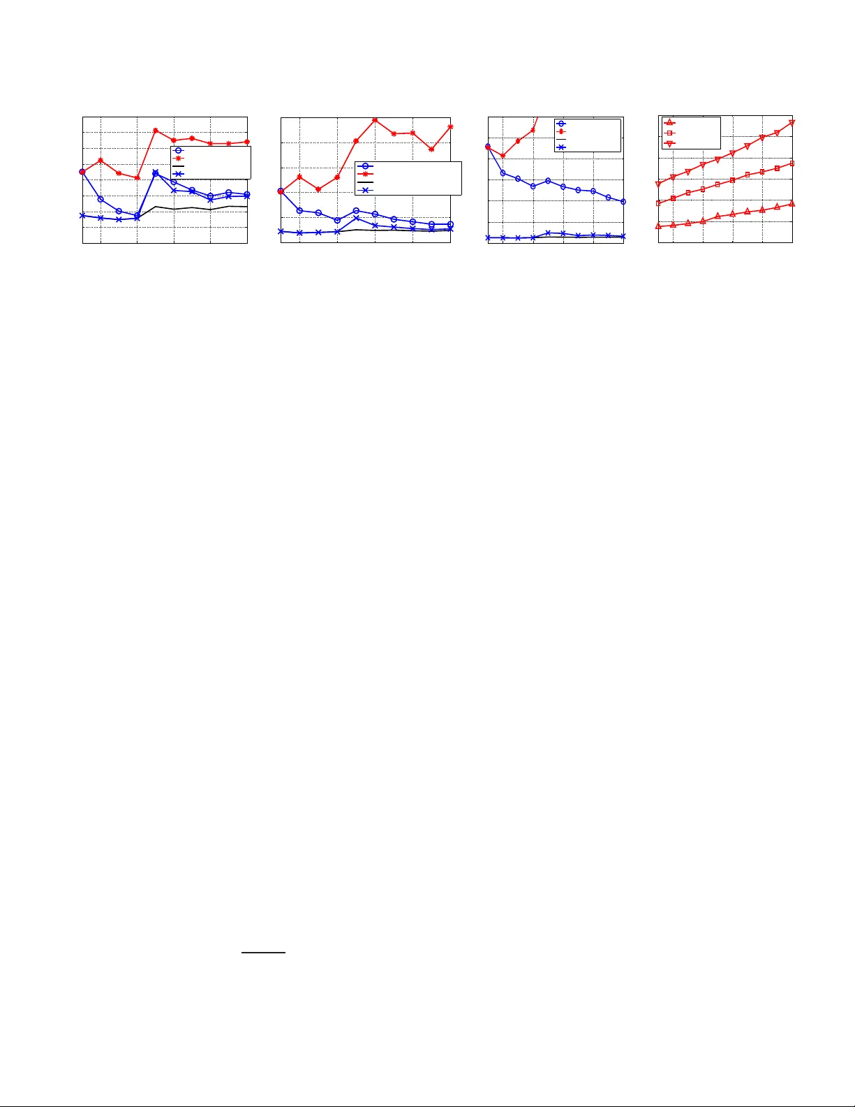
KALMAN FIL TERED COMPRESSED SENS ING Namrata V aswani Dept. of Electrical and Computer Engineering, Io wa State Uni ver sity , Ames, IA, namrata@iastate.edu ABSTRA C T W e consider the problem of reconstructing time sequences of spa- tially sparse signals (wit h unkno wn and time-varying sparsity pat- terns) from a limited numb er of linear “i ncoher ent” measurements, in r eal-time . The signals are sparse in some tr ansform domain re- ferred to as the sparsity basis. For a single spatial signal, the solu- tion is provided by Compressed Sensing (CS ). The question that we address is, for a sequence of sparse signals, can we do better than CS, if (a) the sparsity pattern of the signal’ s transform coefficients’ vector changes slowly ov er ti me, and (b) a simple prior model on the temporal dynamics of its current non-zero elements is a v ailable. The ov erall idea of our solution is to use C S to estimate the sup- port set of the initial signal’ s transform vec tor . At future times, run a reduced order Kalman filter with the currently esti mated support and estimate new additions to the support set by applyin g CS to the Kalman inno vations or filtering err or (whene ver it is “lar ge”) . Index T erms/K eywords: compressed sensing, Kalman filter- ing, compressi ve sampling, sequential MMSE estimation 1. INTRODUCTION W e consider the problem of reconstructing time sequences of spa- tially sparse signals (wit h unkno wn and time-varying sparsity pat- terns) from a limited numb er of linear “i ncoher ent” measurements, in r eal-time . The signals are sparse in some tr ansform domain re- ferred to as t he “sparsity basis” [ 1]. A common example of such a problem is dynamic MRI or CT to image deforming human organs such as the be ating heart or to image brain neural acti v ation patterns (in resp onse to stimuli) usin g fMRI. The ability to perfo rm real-time MRI capture and rec onstruction can mak e interven tional MR practi- cal [2]. Human orga n images are usually piece wise smoo th and thus the wa velet transform i s a v alid sparsity basis [1, 3]. Due to strong temporal dependencies, the sparsity pattern usually changes slowly ov er time. MRI captures a small (sub-Nyquist) number of Fourier transform coef ficients of the image, which are known to be “inco- herent” with respect to the w av elet transform [1, 3]. Other examples include sequentially estimating optical flo w of a single deforming object (sparse in Fourier d omain) from a set of randomly sp aced op- tical flo w measurements (e.g. those at h igh intensity v ariation po ints [4]), or real-time vide o recon struction using single-pix el camera [5]. The solution to the static version of the above problem is pro- vided by Compressed S ensing (CS ) [1, 6, 7]. The noise-free ob- serv ations case [1] is exact with high proba bility (w .h.p.) while the noisy case [7] ha s a small error w .h.p.. But e xisting solutions for the dynamic p roblem [5, 8] t reat the entire time se quence as a single spa- tiotemporal signal and perform CS to reconstruct it. This is a batch solution (need to wait to get the entire observ ati on sequ ence) an d has very high complexity . An alternativ e would be to apply CS at each time separately , which is online an d lo w-complex ity , but will requ ire many more measurements to achiev e low error ( see Fig. 1). The question that we address is: can we do better than performing C S at each time separately , if (a) the sparsity pattern (support set) of the transform coefficien ts’ vector chan ges slowly , i.e. e very time, none or only a few e lements of the suppo rt chang e, and (b) a simple prior model on t he temporal dynamics of it s curr ent non-zer o elements is available (but d o not know which coor dinates are no n-zer o). Our solution is motiv ated by r eformulating the above problem as causal minimum mean squared error (MMSE) estimation with a slo w time-varying set of dominant basis directions (or equiv alently the support of the transform vector). If the support is kno wn, the MMSE solution is give n by the Kalman fi lter ( KF) [9] for this sup- port. But what h appens if the support is unkno wn and time-varying? The initial supp ort can be estimated using CS [7]. I f at a gi ven time, there is an addition to the support set, but we run the KF for the old model, there will be a model mismatch and the innov ation (and fil- tering) error will i ncrease. W hene ver it does , the c hang e in support can be estimated by running CS on the innov ation or the filtering err or , follo wed by t hresholding. A Kalman update step is run using the new support set. If some coefficients become and remain nearly zero (or nearly constant), they can be remo ved from the support set. If, for a moment, we assume that CS [7] giv es the correct esti- mate of the support at all times, then the abov e approach will give the MMSE estimate of the si gnal at all times. The reason it is v ery likely that CS [7] gives the correct estimate i s because we use it to fit a very sparse “model change” signal to the filtering error . Also note that a full Kalman filter [9], that does not use the fact that the signal is sp arse, is meaningless here, because the number of observa- tions av ailable is smaller than the signal dimension, and thus many elements of t he signal transform will be unobserv able. Unless all unobserv able modes are stable, the error w ill blow up. Other re- cent work that also attempts to use prior kno wledge with CS , but to reconstruct only a single signal is [10, 11, 12]. 2. THE MODEL AND PROBLEM FORMULA TION Let ( z t ) m × 1 denote the spatial signal of interest at time t and ( y t ) n × 1 , wi th n < m , denote its observ ation ve ctor at t . The signal, z t , i s sparse in a giv en sparsity basis (e.g. wav elet) wit h orthonormal basis matrix, Φ m × m , i.e. x t , Φ ′ z t is a sparse vec- tor (only S t << m elements of x t are non-zero). Here ′ denotes transpose. The o bserv ations are “incoherent” w .r .t. t he sparsity b asis of the si gnal, i.e. y t = H z t + w t = H Φ x t + w t , where H n × m is such that the correlation between the columns of A , H Φ is small enou gh to ensu re that any S t -column sub-ma trix of A is “ap- proximately orthonormal” (its nonzero singular va lues are between √ 1 − δ to √ 1 + δ for δ < 1 ). w t is the measurement noise. Thus the measurement model is: y t = Ax t + w t , A , H Φ , w t ∼ N (0 , σ 2 obs I ) (1) with w t being temporally i.i.d.. W e refer to x t as the state at t . Our goal is to get the “best” cau sal estimate of x t (or equ i v alently of z t = Φ x t ) at each t . Let T t denote the t he support set of x t , i.e. the set of its non- zero coordinates and let S t = siz e ( T t ) . In other word s, T t = [ i 1 , i 2 , . . . i S t ] where i k are the non-zero coordinates of x t . For any set T , let ( v ) T denote the siz e ( T ) length sub-vector containing t he elements of v corresponding to the indices i n the set T . For another set, γ , we also use the notation T γ which treats T as a vector and selects the elements of T corresponding to t he indices in the set γ . For a matrix A , A T denotes the sub-matrix obtained by extracting the columns of A corresponding to t he indices in T . W e use the no- tation ( Q ) T 1 ,T 2 to denote t he sub-matrix of Q containing rows and columns correspo nding to the entries in T 1 and T 2 respecti vely . T he set operations ∪ , ∩ , and \ have the usual meanings (note T 1 \ T 2 denotes elements of T 1 not in T 2 ). W e use ′ to denote transpose. T c denotes the complement of T w .r .t. [1 : m ] , i.e. T c , [1 : m ] \ T . Also || v || p is the l p norm of the vector v , i.e. || v || p , ( P i | v i | p ) 1 /p . Assumption 1. W e assume sl o w changes in sparsity patterns, i.e. the maximum size of the change in the support set at any time is smaller (usually much smaller) than S t at any t , i.e. S dif f,max , max t [ siz e ( T t \ T t − 1 ) + s iz e ( T t − 1 \ T t )] < min t S t . This, as we shall see later, ensures that performing CS in Gaussian noise to only estimate the additions to the support set results i n smaller error w .h.p. than doing CS to estimate the entire T t again. Assumption 2. W e also assume that A satisfies the Uniform Uncertainty Principle (UUP) ( equation 1.6 of [7 ]) at a sp arsity le v el, S max , max t S t . At first thou ght, it may appear that having A satisfy UUP at the smaller level S dif f,max is suf ficient, b ut, it is not. This is because if S t > S dif f,max for some t , ev en though A T t is a tall matrix, there is no guarantee that at l east S t of its columns are linearly i ndepende nt, i. e. it may happen that r ank ( A T t ) < S t . I n this case, the system no longer r emains observ able for some elements of x t . If any of these elements follo w an unstable prior dy namic model, the KF error will increase unbou ndedly wit h t . System Model for x t . For the currently non -zero coefficients of x t , we assume a spatially i.i.d. Gaussian random walk model, with noise v ariance σ 2 sy s . At the first time instant at which ( x t ) i becomes non-zero, i t is assumed to be generated from a zero mean Gaussian with v ariance σ 2 init . Thus, we hav e the model: x 0 = 0 , ( x t ) i = ( x t − 1 ) i + ( ν t ) i , ( ν t ) i ∼ N (0 , σ 2 sy s ) , if i ∈ T t , i ∈ T t − 1 ( x t ) i = ( x t − 1 ) i + ( ν t ) i , ( ν t ) i ∼ N (0 , σ 2 init ) if i ∈ T t , i / ∈ T t − 1 ( x t ) i = ( x t − 1 ) i if i / ∈ T t (2) The abo ve model can be compa ctly written as: x 0 = 0 , x t = x t − 1 + ν t , ν t ∼ N (0 , Q t ) , ( Q t ) T t ∩ T t − 1 ,T t ∩ T t − 1 = σ 2 sy s I ( Q t ) T t \ T t − 1 ,T t \ T t − 1 = σ 2 init I ( Q t ) T c t ,T c t = 0 (3) where t he set T t is unknown ∀ t . If T t were known at each t , i.e. the system model was completely defined, the MMSE estimate of x t from y 1 , y 2 , . . . y t would be gi ve n by a reduc ed order KF d efined for ( x t ) T t . But, as explained in Sec. 1, i n most practical problems, T t is i n fact unkno wn and time-vary ing. Often, it may be possible to get a rough prior estimate of T 1 by thresholding the eigen values of the co v ariance of x 1 (possible to do if multiple realizations of x 1 are av ailable t o estimate its cova riance). But without multiple i.i.d. realizations of the entire { x t } , which are impossible to obtain in most cases, it i s not possible to get a-priori esti mates of T t for all t . But note that, it i s possible to estimate σ 2 sy s , σ 2 init for the model of (3) using just one “training” realization of { x t } (which is usually easy to get) by setting the near-zero elements to zero in each x t and using the rest to obtain an ML estimate. Assuming kno wn values of σ 2 sy s , σ 2 init , our goal here is to get the best estimates of T t and x t at each t using y 1 , . . . y t . Specifically , 1. At each time, t , get the best estimate of the support set, T t , i.e. get an estimate ˆ T t with smallest p ossible [ siz e ( ˆ T t \ T t ) + siz e ( ˆ T t \ T t )] using y 1 , y 2 . . . y t . 2. Assuming the estimates of T 1 , . . . T t are perfect (have zero error), get the MMSE estimate of x t using y 1 , y 2 . . . y t . 3. KALM AN FIL TERED COMPRESSED SENSING (KF-CS) W e e xplain the proposed KF-CS algorithm belo w . Running the KF . Assume, for no w , that the support set at t he first t ime instan t, T 1 , is known . Consider the situation where t he first change i n the support occurs at a t = t a , i.e. for t < t a , T t = T 1 , and that the change is an addition to the support. This means that for t < t a , we need to just run a regular KF , which assumes the follo wing reduced order measurement and system models: y t = A T ( x t ) T + w t , ( x t ) T = ( x t − 1 ) T + ( ν t ) T , wit h T = T 1 . The KF prediction step for this model is [9]: ˆ x t | t − 1 = ˆ x t − 1 ( P t | t − 1 ) T ,T = ( P t − 1 ) T ,T + σ 2 sy s I (4) with initialization ˆ x 0 = 0 , P 0 = 0 . The update step is [9]: K , ( P t | t − 1 ) T ,T A ′ T Σ − 1 ie , Σ ie , A T ( P t | t − 1 ) T ,T A ′ T + σ 2 obs I ( ˆ x t ) T = ( ˆ x t | t − 1 ) T + K [ y t − A ˆ x t | t − 1 ] ( ˆ x t ) T c = ( ˆ x t | t − 1 ) T c = ( ˆ x t − 1 ) T c ( P t ) T ,T = [ I − K A T ]( P t | t − 1 ) T ,T (5) Note the update step for the elements of T c . Detecting If Addition to Support Set Occurr ed. The Kalman innov ation error is ˜ y t , y t − A ˆ x t | t − 1 . For t < t a , ˜ y t = A ( x t − ˆ x t | t − 1 ) + w t ∼ N (0 , Σ ie ) [9]. At t = t a , a ne w set, ∆ , gets added to t he su pport of x t , i.e. y t = A T ( x t ) T + A ∆ ( x t ) ∆ + w t , where the set ∆ is unkn o wn. Since the old model is used f or t he KF prediction, ˜ y t at t = t a will hav e non-zero mean, A ∆ ( x t ) ∆ , i.e. at t = t a , ˜ y t = A ∆ ( x t ) ∆ + ˜ w t , ˜ w t , [ A T ( x t − ˆ x t | t − 1 ) T + w t ] ∼ N (0 , Σ ie ) (6) Thus, the problem o f detecting if a new set has been added or not gets transformed into the problem of detecting if the Gaussian distributed ˜ y t has non-zero or zero mean. W e use the well-known generalized Likelihood Ratio T est for this problem, which detects i f the weighted innov ation error norm, I E N , ˜ y ′ t Σ − 1 ie ˜ y t ≷ thresh old. One can replace I E N by the weighted norm of the filtering error, defined belo w , which will make the detection more sensiti ve. Estimating the Additions (using CS). If the I E N (or F E N ) is “high” ( abov e the detection threshold), there is a need to estimate ∆ . At t = t a , the inno v ation error , ˜ y t , can also be written as: ˜ y t = A T c ( x t ) T c + ˜ w t , ˜ w t ∼ N (0 , Σ ie ) (7) while the filtering error , ˜ y t,f , y t − A ˆ x t , can be written as: ˜ y t,f = A T c ( x t ) T c + A T ( x t − ˆ x t ) T + w t = [ I − A T K ] A T c ( x t ) T c + ˜ w t,f , ˜ w t,f , [ I − A T K ] ˜ w t ˜ w t,f ∼ N (0 , Σ f e ) , Σ f e , [ I − A T K ]Σ ie [ I − A T K ] ′ (8) Algorithm 1 Kalman Filtered Compressi ve Sensing (KF-CS) Initialization: Set ˆ x 0 = 0 , P 0 = 0 , T 0 = empty (if unkno wn) or equal to the known/partially kno wn support. For t > 0 , do, 1. Set T ← T t − 1 . 2. KF prediction. Run (4 ) using the current T . 3. KF update. Run (5) using the current T . 4. Addition (using CS). Compute I E N = ˜ y ′ t Σ − 1 ie ˜ y t where ˜ y t , y t − A ˆ x t | t − 1 (or compute F E N = ˜ y ′ t,f Σ − 1 f e ˜ y t,f where ˜ y t,f , y t − A ˆ x t ), and check if it is greater than its threshold. If it is, (a) Run CS on the filtering err or , ˜ y t,f , y t − A ˆ x t , i.e. compute the Dantzig selector using (9). (b) Compute the support set of x new by thresholding, i. e. compute nz = { i : | ( x new ) i | > α } . Then the addition to the support set of x t is ∆ = ( T c ) nz . The new suppo rt set for x t is T new = T ∪ ∆ . (c) Set ( P t | t − 1 ) ∆ , ∆ = σ 2 init I . Set T ← T new . (d) Run the KF update gi ven in (5) for the curren t T . Performance can be improv ed by iterating the abov e four steps until siz e (∆) = 0 or F E N less than its threshold. 5. Deletion. Compute the set ∆ D = { i ∈ T : P t τ = t − k +1 ( ˆ x τ ) 2 i < k α 2 } . T he ne w support set is T new = T \ ∆ D . (a) Set ( P t | t − 1 ) ∆ D , [1: m ] = 0 , ( P t | t − 1 ) [1: m ] , ∆ D = 0 . Set T ← T new . 6. KF update. Run (5) for the current T . 7. Assign T t ← T . Output T t , ˆ x t and the signal estimate, ˆ z t = Φ ˆ x t . Increment t and go to step 1. with ( x t ) T c being a sparse vector with support, nz , s.t. ∆ = ( T c ) nz . Note t hat Σ f e < Σ ie . The problem of estimating ( x t ) T c from either ˜ y t or ˜ y t,f is the p roblem of compresse d sen sing i n Gaussian noise studied i n [ 7], excep t that the noise no w is spatially colored. It is not immediately clear whether to use ˜ y t or ˜ y t,f . In ˜ y t,f , the “noise”, ˜ w t,f , is smaller (the chan ge ( x t − x t − 1 ) T has been estimated and subtracted out), but the new component, A T c ( x t ) T c , is also partially suppressed. But the sup pression is small because A T K A T c ( x t ) T c = A T ( P − 1 t | t − 1 σ 2 obs + A ′ T A T ) − 1 A ′ T A T c ( x t ) T c (follows by re writing K using matrix inv ersion lemma [9]) and A ′ T A T c ( x t ) T c = A ′ T A ∆ ( x t ) ∆ is small (since A satisfies UUP at lev el S max and S t a = siz e ( T ∪ ∆) ≤ S max ). Thus, we use ˜ y t,f . The Dantzig selector [7] can be applied to ˜ y t,f to estimate ( x t ) T c , followed by using thresholding to compute its support, nz , and thus get ∆ . Since ˜ w t,f is colored, one way to modify the Dantzig selector to apply it to (8) is to compute: x new =arg min β || β || 1 , s.t. || A ′ T c Λ − 1 / 2 U ′ [ ˜ y t,f − A T c β ] || ∞ ≤ λ m (9) where Σ f e = U Λ U ′ is the eigen value decomposition of Σ f e and λ m , √ 2 log m trace (Σ f e ) /n . The set nz is estimated as nz = { i : | ( x new ) i | > α } for some zeroing threshold α and the set ∆ is ∆ = ( T c ) nz . T hus the new support set i s T new = T ∪ ∆ . W e initialize the prediction cov ariance along ∆ : ( P t | t − 1 ) ∆ , ∆ = σ 2 init I . KF Update. W e run the KF update gi ven in (5) with T = T new . This can be interpreted as a Bayesian v ersion of Gauss-Dantzig [7]. Iterating CS and KF -update . Oft en, it may happen that not all the elements of the true ∆ get estimated i n one run of the CS step, because of t he error i n CS. T o address t his, the abov e steps (CS and KF update) can be iterated until F E N goes belo w a threshold or un- til t he estimated set ∆ is empty or for a fixed number of it erations. A similar idea forms the basis of iterati v e CS recon struction techniques such as stage wi se Orthogonal Matching Pursuit[13]. Deleting N ear-Zer o Coefficients. Over time, some coefficients may become zero (or nearly-zero) and remain zero. Alt ernativ ely , some coefficients may wrongly get added, due t o C S error . In both cases, the coefficients need to be r emov ed from the support set T t . A simple w ay to do this wo uld be to check if | ( ˆ x t ) i | < α ( α is a zeroing threshold) for a few time instants. When a coefficient is remov ed, the correspon ding row and column in P t | t − 1 is set to zero. Deleting Constant Coefficients. If a coefficient, i , becomes nearly-constant ( this may happen in certain applications), one can keep improving the estimate of its constant value by changing the prediction step for it to ( P t | t − 1 ) i,i = ( P t − 1 ) i,i . Either o ne can keep doing this forev er (the error in its estimate will go to zero with t ) or one can assume t hat the esti mation error has become negligibly small after a finite time and then remov e the coef ficient i ndex from T t . The bias-variance tradeoff needs to be ev aluated before select- ing either scheme. If the latter is done, then for future t imes, one needs to replace y t by y t − A i ( ˆ x ) i and set ( P t | t − 1 ) i, [1: m ] = 0 , ( P t | t − 1 ) [1: m ] ,i = 0 . This will be part of future work. Initialization. Initially , the support set, T 1 may be roughly kno wn (estimated by thresholding t he eigen v alues of the cov ariance of x 1 , which is computable if its multiple realizations are ava ilable) or unkno wn. W e initi alize KF-CS by setting ˆ x 0 = 0 , P 0 = 0 and T 0 = rou ghly kno wn support or T 0 = empty (if support is completely unkno wn). In the latter case, automatically at t = 1 , the I E N (or F E N ) will be large, and thus CS will run to estimate T 1 . The entire KF-CS algorithm is summarized in Algorithm 1. 3.1. Discussion The key difference between KF -CS and regular CS at each t is that KF-CS performs C S on the filtering err or , ˜ y t,f , to only detect new additions while regular CS performs CS on the observation, y t , t o detect the entire vector x t (without using knowledge of the previ- ous support set). From [7, Theorem 1.1] (the result should hold di- rectly or with slight modification for CS in colored noise, but we hav e not checked it yet), t he C S error is directl y proportional to the sparsity size of the vector being estimated and to the noise v ariance. But t he dependen ce on sparsity size is much stronger (highly non- linear) while that on the noise variance is l inear . Note that “CS on filtering error” needs to estimate at most S dif f, max coef ficients and S dif f, max < S t , ∀ t (Assumption 1). Thus, i f the “noises” in both 2 4 6 8 10 0 0.05 0.1 0.15 0.2 0.25 0.3 0.35 0.4 Time MSE S max = 8 CS−KF−T1−Unknown Regular CS Genie−aided KF CS−KF−T1−Known 2 4 6 8 10 0 1 2 3 4 5 Time MSE S max = 16 CS−KF−T1−Unknown Regular CS Genie−aided KF CS−KF−T1−Known 2 4 6 8 10 0 5 10 15 20 25 30 Time MSE S max = 25 CS−KF−T1−Unknown Regular CS Genie−aided KF CS−KF−T1−Known 2 4 6 8 10 0 50 100 150 200 250 300 Time MSE MSE of Full KF Full KF, S=8 Full KF, S=16 Full KF, S=25 Fig. 1 . MSE plots of KF -CS (labeled CS-KF i n the plots), T 1 unkno wn and kno wn cases, compared against regular CS in the first 3 fi gures and against the Full 256-dim K F in t he last figure (its MSE i s so large that we cannot plot it in the same scale as the others). The benchmark (MMSE estimate with kno wn T 1 , T 5 ) is the genie-aided KF . The simulated signal’ s energ y at t is E [ || x t || 2 2 ] = S 1 σ 2 init + ( P t τ =2 S τ ) σ 2 sy s ) . cases were the same, then the err or in “CS on filtering error” would be much smaller than that in CS. But the “noise” in y t is only w t , while the “noise” in ˜ y t,f is w t plus A T ( x t − ˆ x t ) T . If we can show stability of KF- CS err or , and if the temporal prior is strong enough, the cov ariance of this extra “noise” wi ll be small enough. Thus, it should be possible to sho w that the error in KF-CS is smaller than that in re gular CS, if the spa rsity pattern chang es slowly e nough and the temporal prior is strong enough . A rigorous comparison of KF -CS with CS and an analy sis of KF-CS error stability wi ll be part of future work. W e provide here a qualitativ e discussion of the sources of error in KF-CS . The error can be du e t o two reasons - either the CS step misses some non- zero coef ficients (or the deletion step wrongly deletes a non-zero coef ficient) or the CS step estimates some extra coefficients (or the deletion step misses remov ing some coef ficients). Occasionally , an element, i , of t he tr ue ∆ may get missed, due to nonzero CS error (or the thresholding error). The extra error due to an ( x t ) i getting missed cannot be larger than the C S error at the current ti me ( which itself is upper bounded by a small v alue w .h.p. [7]) plus α (due to thresholding). Also, ev entually , when the mag- nitude of ( x t ) i increases at a future time, it will result in a “high” I E N and F E N , and the CS step at t hat time will estimate it w . h.p.. W e can pre ve nt t oo many extra coordinates from getting wrongly estimated b y ha ving a ro ugh idea of the maximum sp arsity o f x t and using thresholding to only select t hat many , or a few more, highest magnitude non-zero elements. The deletion threshold also needs to be selected appropriately . Also, if, because of CS thresholding or deletion, some true element gets missed because its value was too small, it will, w .h.p., get detected b y CS at a future time when I E N increases. Also, as long as r ank ( A T ) > siz e ( T ) for the currently estimated T (which may contain some extra coordinates), the esti- mation error wi ll increase beyond MMSE, but will not blow up, i.e. it will still con verge, b ut to a higher constant v alue. 4. SIMULA TION RESUL TS W e simulated a time sequence of sparse m =256 length signals, x t , with maximum sparsity S max . T hree sets of simulations were run with S max = 8, 16 and 25. The A matri x was simulated as i n [7] by generating n × m i.i .d. Gaussian entries (with n = 72 ) and normal- izing each column of the resulting matri x. Such a matrix has been sho wn to satisfy the UUP at a lev el C log m [7]. The observ ation noise varian ce, σ 2 obs = ((1 / 3) p S max /n ) 2 (this is t aken from [7]). The prior model on x t was (3) with σ 2 init = 9 and σ 2 sy s = 1 . T 1 (support set of x 1 ) was obtained by generating S max − 2 unique in- dices uniformly randomly fr om [1 : m ] . W e simulated an increase in the support at t = 5 , i.e. T t = T 1 , ∀ t < 5 , while at t = 5 , we added two more elements to the support set. T hus, T t = T 5 , ∀ t ≥ 5 had size S max . Only addition to the support was simulated. W e used the proposed KF-CS algorithm (Algorithm 1) to com- pute the causal estimate ˆ x t of x t at each t . The resulting mean squared error (MSE) at each t , E x,y [ || x t − ˆ x t || 2 2 ] , was computed by av eraging o v er 100 Monte Carlo simulations of the abov e model. The same matrix, A , w as used in all the simulations, b ut we averaged ov er the joint p df of x, y , i.e. we generated T 1 , T 5 , ( ν t ) T t , , w t , t = 1 , . . . 10 randomly in each simulation. Our simulation results are sho wn i n Fi g. 1 (KF-CS is labeled as CS-KF in plots by mistake) . Our b enchmark was the g enie-aided KF , i.e. an S max -order KF with kno wn T 1 and T 5 , which generates the MMSE estimate of x t . W e simulated two t ypes of KF-C S methods, one with kno wn T 1 , b ut un - kno wn T 5 and the other with unknown T 1 and T 5 . Both performed almost e qually well for S max = 8 , but as S max was i ncreased mu ch beyo nd the UU P level of A , the performance of the unknown T 1 case degrad ed more (the CS assumption did not hold). W e also show comparison with r egular CS at each t , which does not use the fact that T t changes slo wly (and does not assum e kno wn T 1 either). This had much higher MSE than KF -CS. The MSE beco me worse for larger S max . W e also implemented the full KF for the 256 -dim state vector . This used (3) wi th Q t = σ 2 sy s I 256 × 25 6 , i.e. it assumed no kno wl edge of the sparsity . Since we had only a 72-length obser- v ation vector , the full system i s not observ able. Si nce all non-zero modes are unstable, its error blo ws up. 5. CONCLUSIONS AND FUTURE DIRECTIONS T o the best of our kno wledge, this is the first work on extending the C S i dea to causally estimate a time sequence of spatially sparse signals. W e do this by using CS to estimate the signal support at t he initial t ime instant, followed by running a KF for the reduced order model, until the inno v ation or filtering erro r increases. When it does, we estimate t he “change i n support” by running CS on t he filtering error . This has much lo wer error since the “change ” i s much sparser than the actual signal. Open questions to be addressed in future are (a) the analysis of t he stability of KF-C S, (b) comparison of KF-CS error wit h that of regular CS, (c) studying ho w and when to delete constant coefficients, (d) KF -CS for compressible signal sequences, and (e) its exten sions to large-dimensiona l particle fi ltering [14]. 6. REFERENCES [1] E. Candes, J. Romberg , and T . T ao, “Robust uncertainty princi- ples: Exact signal reconstruction from highly incomplete fre- quenc y information, ” IEEE T rans. Info. Th. , vol. 52(2), pp. 489–50 9, February 2006. [2] A. J. Martin, O. M. W eber , D. Saloner , R. Higashida, M. Wil- son, M. Saeed, and C.B. Higgins, “ Application of mr tech- nology to endo v ascular interventions in an xmr suite, ” Medica Mundi , vo l. 46, December 2002. [3] M. Lustig, D. D onoho, and J. M. Pauly , “S parse mri: The ap- plication of compressed sensing for rapid mr imaging, ” Mag- netic Resonance i n Medicine , vol. 58(6), pp. 1182–1195 , De- cember 2007. [4] Jianbo Shi and Carlo T omasi, “Good features to track, ” in IEEE Conf. on Comp. V is. and P at. Recog. (CV PR) , 1994, pp. 593–60 0. [5] M. W akin, J. Laska, M. Duarte, D. Baron, S . Sarv otham, D. T akhar , K. Kelly , and R. Baraniuk, “ An architecture for compressi v e i maging, ” in I EEE Intl. Conf. on Imag e P r ocess- ing , 2006 . [6] D. Donoho, “Compressed sensing, ” IEEE T rans. on Informa- tion Theory , vol. 5 2(4), pp. 1289–1 306, April 2006. [7] E. Candes and T . T ao, “The dantzig selector: statistical esti- mation w hen p is much larger than n, ” Annals of Statistics , 2006. [8] U. Gamper , P . Boesiger , and S. Koze rke, “Compressed sensing in d ynamic mri, ” Magnetic Resona nce in Med icine , vo l. 59(2), pp. 365–37 3, January 2008. [9] T . Kailath, A.H. S ayed, and B. Hassibi, Linear Estimati on , Prentice Hall, 2000. [10] J. Garcia-Fri as and I. Esnaola, “Exploiting prior knowledge in the recovery of signals from noisy random projections, ” in Data Compr ession C onfer ence , 2007. [11] K. Egiazarian, A. Foi, and V . Katko vnik, “Compressed sensing image recon struction via recursi ve spatially adapti ve filtering, ” in IEEE Intl. Conf. on Ima ge Pr ocessing , 2007. [12] S . Ji, Y . Xue, and L. Cari n, “Bayesian compressi ve sensing, ” IEEE T rans. Sig. Pr oc. , to appear . [13] D. L. Donoho, Y . T saig, I. Drori, and J-L. Starck, “Sparse solu- tion of underdetermined linear equations by stage wise orthog- onal matching pursuit, ” IEEE T ra ns. on Information Theory , (Submitted) 2007 . [14] N. V asw ani, “Particle filters for infinite (or l arge) dimensional state spaces-part 2, ” in IEEE Intl. Con f. Acoustics, S peec h, Sig . Pr oc. (ICASSP) , 20 06.