On the Relationship between Transmission Power and Capacity of an Underwater Acoustic Communication Channel

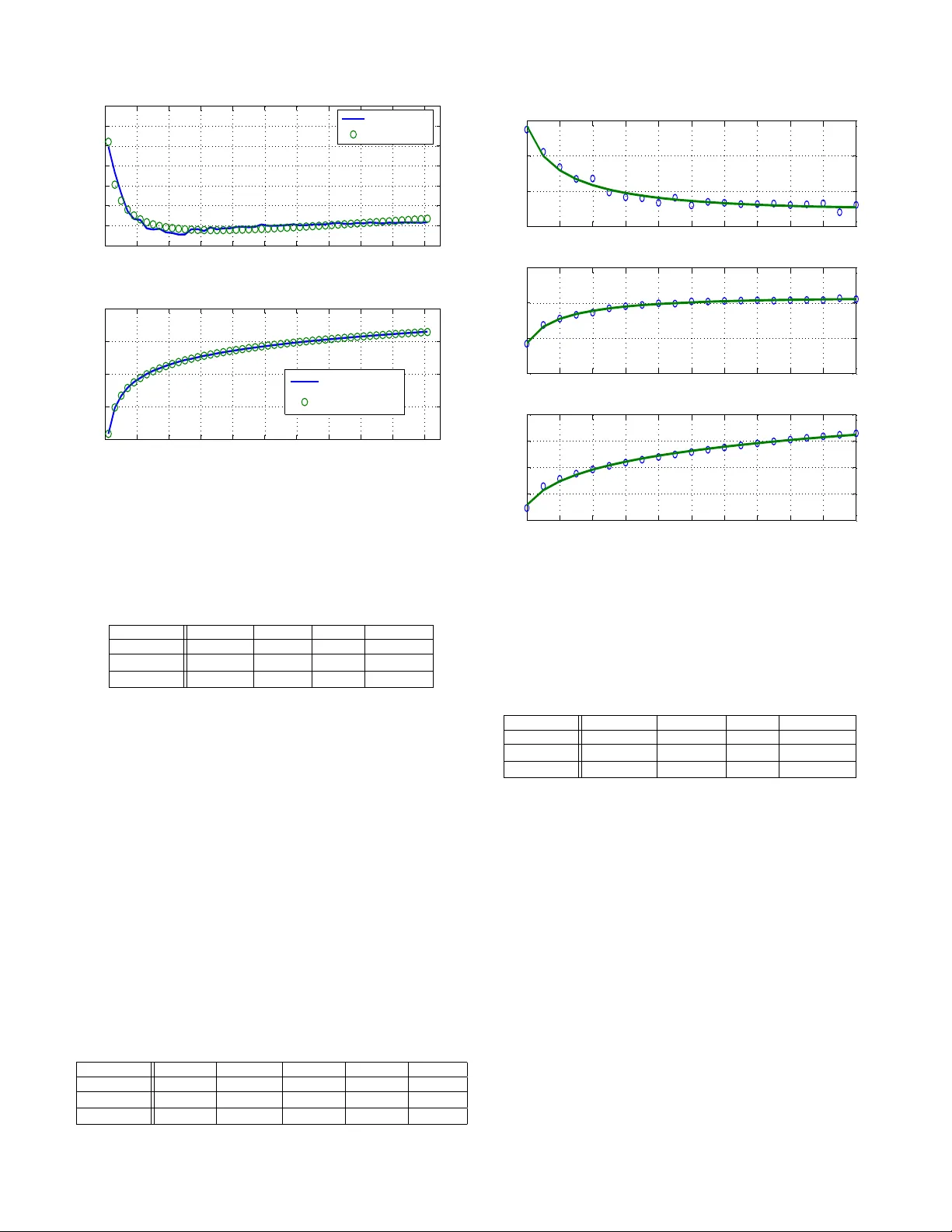
On the Relationship between T ransmission Po wer and Capacity of an Underwater Acoustic Communication Channel Daniel E. Lucani LIDS, MIT Cambridge, Massachusetts, 02139 Email: dlucani@mit.edu Milica Stojanovic MIT Cambridge, Massachusetts, 02139 Email: millitsa@mit.edu Muriel M ´ edard LIDS, MIT Cambridge, Massachusetts, 02139 Email: medard@mit.edu Abstract — The underwater acoustic channel is characterized by a path loss that depends not only on the transmission distance, but also on the signal frequency . As a consequence, transmission bandwidth depends on the transmission distance, a feature that distinguishes an underwater acoustic system from a terrestrial radio system. The exact relationship between po wer , transmission band, distance and capacity for the Gaussian noise scenario is a complicated one. This work provides a closed-form approximate model for 1) power consumption, 2) band-edge frequency and 3) bandwidth as functions of distance and capacity required for a data link. This approximate model is obtained by numerical evaluation of analytical results which takes into account physical models of acoustic propagation loss and ambient noise. The closed-form approximations may become useful tools in the design and analysis of underwater acoustic networks. I . I N T R O D U C T I O N W ith the advances in acoustic communication technology , the interest in study and experimental deployment of under - water networks has been growing [1]. Ho wev er , underwater acoustic channels impose man y constraints that af fect the design of wireless networks. They are characterized by a path loss that depends on both the transmission distance and the signal frequency , a feature that distinguishes an underwater acoustic system from a terrestrial radio system. Thus, not only the po wer consumption, b ut also the useful bandwidth depend on the transmission distance [2]. From an information theoretic perspective, both the distance between two nodes and the required capacity determine the power consumption for that link and the optimal transmission band. It is thus of interest to have a simple, closed-form expression that relates the transmission power to the desired capacity . This would enable an efficient design of both point to point links and underwater networks, ev entually leading to a minimum cost overall network optimization. Thus, these expressions may be useful from both a theoretic and an engineering standpoint. In this paper , simple closed-form approximations for the power consumption and operating frequency band as functions of distance and capacity are presented. This approximate model stems from an information theoretic analysis that takes into account a physical model of acoustic propagation loss, and colored Gaussian ambient noise. It was shown in [2] that the transmission power as a function of the distance could be well approximated by P ( l ) = pl γ . A similar relationship was shown to exist for the operating bandwidth. The coef ficients in this model were determined as functions of the required signal to noise ratio. The present work extends this idea of modeling the power and bandwidth as functions of distance, but the problem is cast into a slightly dif ferent frame work. Namely , instead of using the SNR as a constraint, i.e. a fix ed design parameter , the desired link capacity is used as a figure of merit. In few words, this work proposes approximate models for the parameters as functions of the capacity . This resulting model is useful for a broad range of capacities and distances. The paper is organized as follows. In Section 2, a model of an underwater channel is outlined. In Section 3, a brief description of the numerical ev aluation procedure is described. In Section 4, closed-form expressions for the parameters of interest are presented. Section 5 gives numerical results for different ranges of distance and capacity . Conclusions are summarized in the last section. I I . C H A N N E L M O D E L An underwater acoustic channel is characterized by a path loss that depends on both distance l and signal frequency f as A ( l, f ) = l k a ( f ) l (1) where k is the spreading factor and a ( f ) is the absorption coefficient [2]. The spreading factor describes the geometry of propagation, e.g. k = 2 corresponds to spherical spreading, k = 1 to cylindrical spreading, and k = 1 . 5 to practical spreading. The absorption coef ficient can be expressed in dB/km using Thorp’ s empirical formula for f in kHz: 10 log a ( f ) = 0 . 11 f 2 1 + f 2 + 44 f 2 4100 + f 2 + 2 . 75 · 10 − 4 f 2 + 0 . 003 (2) A(l,f)N(f) f K (n) (l,C) K (n+1) (l,C) f o ε f (n) end f (n) ini () ˆ n B ^ ^ Fig. 1. Numerical procedure for computation of P ( l, C ) , ˆ f end ( l, C ) and ˆ B ( l, C ) , by incrementing K ( l, C ) at each step by  until a stopping condition is fulfilled for frequencies abov e a fe w hundred Hz. For lower frequen- cies, the model is: 10 log a ( f ) = 0 . 11 f 2 1 + f 2 + 0 . 011 f 2 + 0 . 002 (3) The noise in an acoustic channel can be modeled through four basic sources: turbulence, shipping, waves, and thermal noise[2]. The following formulas give the po wer spectral density (psd) of these noise components in dB re µ Pa per Hz as a function of frequency in kHz: log N t ( f ) = 1 . 7 − 3 log f (4) log N s ( f ) = 4 + 2( s − 1 2 ) + 2 . 6 log f − 6 log ( f + 0 . 03) (5) log N w ( f ) = 5 + 0 . 75 w 1 / 2 + 2 log f − 4 log( f + 0 . 4) (6) log N th ( f ) = − 1 . 5 + 2 log f (7) where the shipping activity s ranges from 0 to 1, for lo w and high activity , respectiv ely , and w corresponds to the wind speed measured in m/s. The overall psd of the ambient noise is giv en by N ( f ) = N t ( f ) + N s ( f ) + N w ( f ) + N th ( f ) (8) Let us assume that this is a Gaussian channel. Then, the capacity of this channel can be obtained using the waterfilling principle [2]. Also, assume that the power and band of operation can be adjusted to reach a certain capacity level. Thus, the capacity of a point-to-point link is C = Z B ( l,C ) log 2  K ( l , C ) A ( l, f ) N ( f )  d f (9) 0 0.2 0.4 0.6 0.8 1 1.2 1.4 1.6 1.8 2 2.46 2.47 2.48 2.49 2.5 2.51 Capacity [kbps] 0 0.2 0.4 0.6 0.8 1 1.2 1.4 1.6 1.8 2 50 55 60 65 70 75 80 Capacity [kbps] Parameter a 1 (C) Approximate a 1 (C) Parameter a 2 (C) Approximate a 2 (C) Fig. 2. Parameters a 1 and a 2 for P ( l , C ) and approximate model. l ∈ [0 , 10 km ] , C ∈ [0 , 2 kbps ] , k = 1 . 5 , s = 0 . 5 and w = 0 m/s where B ( l, C ) is the optimum band of operation. This band could be thought of as a union of non-overlapping intervals, B ( l, C ) = ∪ i [ f i ini ( l, C ) , f i end ( l, C )] , where each non-ov erlapping band i has the lower -end frequency f i ini ( l, C ) and the higher -end frequency f i end ( l, C ) associated to it. In its simplest form B ( l, C ) = [ f ini ( l, C ) , f end ( l, C )] . The power consumption associated with a particular choice of ( l, C ) is given by P ( l, C ) = Z B ( l,C ) S ( l , C, f ) d f (10) where S ( l , C, f ) = K ( l , C ) − A ( l, f ) N ( f ) , f ∈ B ( l, C ) . Evidently , these expressions are quite complicated to be used in a computational network analysis. Also, the y provide little insight into the relationship between power consumption, ˆ f ini and ˆ f end , in terms of the pair ( l , C ) . This motiv ates the need for an approximate model that will represent these relations for ranges of C and l that are of interest to acous- tic communication systems. The model should also provide flexibility to changing other parameters, such as the spreading factor k , wind speed w and shipping activity s . The dependence on the spreading factor k is quite simple. Let us assume that a model for P ( l , C ) has been de veloped for a particular value of k = k i , i.e. P ( l , C, k i ) . T o determine P ( l, C , k j ) for k j 6 = k i , let us note that for a change in k , the product A ( l, f ) N ( f ) = l k a ( f ) l N ( f ) constitutes a constant scaling f actor with respect to f . Therefore, for a link of distance l the term B ( l, C ) will remain unchanged. Thus, if the same capacity C is required for k i and k j , equation (9) shows that the only other term that can vary is K ( l, C ) , 0 0.2 0.4 0.6 0.8 1 1.2 1.4 1.6 1.8 2 -0.48 -0.47 -0.46 -0.45 -0.44 -0.43 Capacity [kbps] 0 0.2 0.4 0.6 0.8 1 1.2 1.4 1.6 1.8 2 12.8 13 13.2 13.4 13.6 13.8 14 Capacity [kbps] Parameter a 1 (C) Approximate a 1 (C) Parameter a 2 (C) Approximate a 2 (C) Fig. 3. P arameters a 1 and a 2 for ˆ f end ( l, C ) and approximate model. l ∈ [0 , 10 km ] , C ∈ [0 , 2 kbps ] , k = 1 . 5 , s = 0 . 5 and w = 0 m/s i.e. K ( l, C, k ) . Then, K ( l , C, k j ) = l k j − k i K ( l , C, k i ) . Finally , let us use the equation (10) to determine the relationship between P ( l , C, k i ) and P ( l , C, k j ) . The dependence on the spreading factor k is quite simple. Let us assume that a model for P ( l, C ) has been dev eloped for a particular value of k = k i , i.e. P ( l, C, k i ) . T o determine P ( l, C, k j ) for k j 6 = k i . Note that for a change in k , the product A ( l, f ) N ( f ) = l k a ( f ) l N ( f ) constitutes a constant scaling factor with respect to f . Therefore, for a link of distance l the term B ( l , C ) will remain unchanged. Thus, if the same capacity C is required for k i and k j , equation (9), shows that the only other term that can v ary is K ( l, C ) , i.e. K ( l , C, k ) . Then, K ( l , C, k j ) = l k j − k i K ( l , C, k i ) . Finally , let us use equation (10) to deter- mine the relation between P ( l, C , k i ) and P ( l, C , k j ) . P ( l, C , k j ) = Z B ( l,C )  K ( l , C, k j ) − l k j a ( f ) l N ( f )  d f (11) = l k j − k i Z B ( l,C )  K ( l , C, k i ) − l k i a ( f ) l N ( f )  d f (12) = l k j − k i P ( l, C , k i ) (13) Thus, any model for the transmission generated for some parameter k has a simple extension. Also, note that the transmission bandwidth remains the same for any value of k . I I I . N U M E R I C A L E V A L U A T I O N P RO C E D U R E A numerical ev aluation procedure similar to that in [2] is used to compute the value of P ( l , C ) , ˆ f ini ( l, C ) and ˆ f end ( l, C ) , for a region of values of ( l , C ) . The procedure 0 0.2 0.4 0.6 0.8 1 1.2 1.4 1.6 1.8 2 -0.3085 -0.308 -0.3075 -0.307 -0.3065 -0.306 -0.3055 -0.305 Capacity [kbps] 0 0.2 0.4 0.6 0.8 1 1.2 1.4 1.6 1.8 2 2 4 6 8 10 12 Capacity [kbps] Parameter a 1 (C) Approximate a 1 (C) Parameter a 2 (C) Approximate a 2 (C) Fig. 4. Parameters a 1 and a 2 for ˆ B ( l, C ) and approximate model. l ∈ [0 , 10 km ] , C ∈ [0 , 2 kbps ] , k = 1 . 5 , s = 0 . 5 and w = 0 m/s starts by fixing a target v alue of the capacity C . Then, for each distance l , the initial v alue of K ( l, C ) is set to the minimum value of the product A ( l , f ) N ( f ) , i.e. K ( l , C ) = min f A ( l, f ) N ( f ) . The frequenc y at which this occurs, i.e. f 0 = arg min f A ( l, f ) N ( f ) , is called the optimal frequency . After this, K ( l , C ) is increased iterati v ely by a small amount (Figure 1), until the target capacity v alue C is met. Finally , this procedure is repeated for each value of C in a range of interest. At the n -th step of the procedure, when K ( n ) ( l, C ) is in- creased by a small amount, the band B ( n ) ( l, C ) is determined for that iteration. This band is defined as the range of fre- quencies for which the condition A ( l, f ) N ( f ) ≤ K ( n ) ( l, C ) . Then, the capacity C ( n ) is numerically determined for the current K ( n ) ( l, C ) and B ( n ) ( l, C ) , using the equation (9). If C ( n ) < C , a new iteration is performed. Otherwise, the procedure stops. I V . A P P R OX I M A T E M O D E L S By applying the above procedure for varying l and C , one arriv ed at the complete model for the po wer consumption P ( l, C ) = 10 a 1 ( C ) 10 l a 2 ( C ) (14) where a 1 ( C ) = β 3 + β 2 10 log 10 C + β 1 (10 log 10 ( C + 1)) 2 (15) a 2 ( C ) = α 3 + α 2 C + α 1 C 2 (16) Below , two ranges of operation were studied. The first one is for l ∈ [0 , 10] k m , C ∈ [0 , 2] k bps , and propagation factor 0 10 20 30 40 50 60 70 80 90 100 2.5 3 3.5 4 4.5 5 5.5 Capacity [kbps] 0 10 20 30 40 50 60 70 80 90 100 65 70 75 80 85 Capacity [kbps] Parameter a 1 (C) Approximate a 1 (C) Parameter a 2 (C) Approximate a 2 (C) Fig. 5. Parameters a 1 and a 2 for P ( l , C ) and approximate model. l ∈ [0 , 100 km ] , C ∈ [0 , 100 k bps ] , k = 1 . 5 , s = 0 . 5 and w = 0 m/s of k = 1 . 5 , which will be called case 1 from here on. The second one is for l ∈ [0 , 100] K ms , C ∈ [0 , 100] k bps , and propagation factor of k = 1 . 5 , which will be called case 2. For both regions and dif ferent ranges of s and w , the power consumption P ( l , C ) can be approximated by equations (14), (15) and (16). Similar model are found to provide a good fit for the high/end frequency ˆ f end ( l, C ) and for the bandwidth ˆ B ( l, C ) = ˆ f end ( l, C ) − ˆ f ini ( l, C ) . These models are giv en by ˆ f end ( l, C ) = 10 a 1 ( C ) 10 l a 2 ( C ) (17) where a 1 ( C ) = β 3 + β 2 10 log 10 C + β 1 (10 log 10 C ) 2 (18) a 2 ( C ) = α 3 + α 2 10 log 10 C + α 1 (10 log 10 C ) 2 (19) ˆ B ( l, C ) = 1 0 a 1 ( C ) 10 l a 2 ( C ) (20) where a 1 ( C ) = β 3 + β 2 10 log 10 C + β 1 (10 log 10 C ) 2 (21) a 2 ( C ) = α 4 + α 3 10 log 10 C + α 2 (10 log 10 C ) 2 + α 1 (10 log 10 C ) 3 (22) V . N U M E R I C A L R E S U LT S The transmission power , highest frequency and bandwidth of transmission band were computed for a variety of values of s , w and two ranges of interest of the pair ( l, C ) , i.e. l ∈ [0 , 10] K ms , C ∈ [0 , 2] k bps , and l ∈ [0 , 100] K ms , 0 10 20 30 40 50 60 70 80 90 100 -0.65 -0.6 -0.55 -0.5 -0.45 -0.4 -0.35 Capacity [kbps] 0 10 20 30 40 50 60 70 80 90 100 14.5 15 15.5 16 16.5 17 Capacity [kbps] Parameter a 1 (C) Approximate a 1 (C) Parameter a 2 (C) Approximate a 2 (C) Fig. 6. P arameters a 1 and a 2 for ˆ f end ( l, C ) and approximate model. l ∈ [0 , 100 km ] , C ∈ [0 , 100 k bps ] , k = 1 . 5 , s = 0 . 5 and w = 0 m/s T ABLE I a 1 A P PR OX I MATI O N PAR A M E TE R V A L UE S F O R P ( l, C ) , ˆ f end ( l, C ) A N D ˆ B ( l, C ) , W I T H l ∈ [0 , 10 km ] , C ∈ [0 , 2 k bps ] , k = 1 . 5 , s = 0 . 5 A N D w = 0 m/s α 1 α 2 α 3 α 4 MSE P ( l, C ) 0 -0.00432 0.02873 2.46560 2.532e-7 ˆ f end ( l, C ) 0 4.795e-5 0.00246 -0.44149 3.930e-9 ˆ B ( l, C ) -5.958e-7 -2.563e-5 -0.000305 -0.30694 6.599e-9 C ∈ [0 , 100] k bps . The models proposed fitted these cases quite well. Results are presented for the case of k = 1 . 5 , w = 0 and s = 0 . 5 , for both cases. Also for case 1, it will be seen that the α and β parameters show almost no dependence on the shipping activity factor s , especially if the wind speed is w > 0 . Thus, the approximate model for this case could be simplified to only consider w as part of the model, instead of the pair ( s, w ) . Figures 2, 3 and 4 sho w parameters a 1 and a 2 for P ( l, C ) , ˆ f end ( l, C ) , and ˆ B ( l, C ) , respectiv ely . This approxi- mation was carried out for the first case with a propagation factor of k = 1 . 5 , a shipping activity of s = 0 . 5 and a wind speed of w = 0 m/s . The values of α ’ s and β ’ s are shown in T able I and II, for parameters a 1 and a 2 , respecti v ely . These tables also sho w the mean square error (MSE) of the approximation with respect to the actual parameters. In Figure 4, there is a considerable v ariation in the values of parameter a 1 ( C ) . Howe ver , note that the y-axis of the plot sho ws very little variation. Figures 5, 6 and 7 sho w parameters a 1 and a 2 for P ( l, C ) , ˆ f end ( l, C ) , and ˆ B ( l, C ) , respectiv ely . This approxi- 0 10 20 30 40 50 60 70 80 90 100 -0.39 -0.385 -0.38 -0.375 -0.37 -0.365 -0.36 -0.355 Capacity [kbps] 0 10 20 30 40 50 60 70 80 90 100 10 12 14 16 18 Capacity [kbps] Parameter a 1 (C) Approximate a 1 (C) Parameter a 2 (C) Approximate a 2 (C) Fig. 7. Parameters a 1 and a 2 for ˆ B ( l, C ) and approximate model. l ∈ [0 , 100 km ] , C ∈ [0 , 100 k bps ] , k = 1 . 5 , s = 0 . 5 and w = 0 m/s T ABLE II a 2 A P PR OX I MATI O N PAR A M E TE R V A L UE S F O R P ( l, C ) , ˆ f end ( l, C ) A N D ˆ B ( l, C ) , W I T H l ∈ [0 , 10 km ] , C ∈ [0 , 2 k bps ] , k = 1 . 5 , s = 0 . 5 A N D w = 0 m/s β 1 β 2 β 3 MSE P ( l, C ) 0.01166 1.0117 72.043 5.8979e-5 ˆ f end ( l, C ) 0.00171 0.07153 13.738 3.4706e-5 ˆ B ( l, C ) -5.163e-6 0.33427 9.6752 2.9233e-7 mation was carried out for the second case with a propagation factor of k = 1 . 5 , a shipping activity of s = 0 . 5 and a wind speed of w = 0 . The values of α ’ s and β ’ s are shown in T able III and IV, for parameters a 1 and a 2 , respecti vely . These tables also sho w the mean square error (MSE) of the approximation with respect to the actual parameters. For both ranges, the proposed models gi ve a very good approximation to the actual numerical values. Also note that for the a 2 ( C ) parameter of P ( l, C ) , it is possible to use a linear approximation, instead of a quadratic model. Let us analyze the lo w range low rate for different v alues of s and w . T able V sho ws the v alues for α and β parameters T ABLE III a 1 A P PR OX I MATI O N PAR A M E TE R V A L UE S F O R P ( l, C ) , ˆ f end ( l, C ) A N D ˆ B ( l, C ) , W I T H l ∈ [0 , 100 km ] , C ∈ [0 , 100 k bps ] , k = 1 . 5 , s = 0 . 5 A N D w = 0 m/s α 1 α 2 α 3 α 4 MSE P ( l, C ) 0 -5.617e-5 0.02855 2.9305 0.00011 ˆ f end ( l, C ) 0 -0.00019 0.01186 -0.55076 1.32e-7 ˆ B ( l, C ) 1.696e-6 4.252e-5 -0.00249 -0.36397 7.29e-7 0 2 4 6 8 10 12 14 16 18 20 -6 -5.5 -5 -4.5 x 10 -3 α 1 0 2 4 6 8 10 12 14 16 18 20 0.025 0.03 0.035 0.04 α 2 0 2 4 6 8 10 12 14 16 18 20 2.5 2.6 2.7 2.8 α 3 Wind Speed (m/s) Fig. 8. V alues of α as function of w . l ∈ [0 , 10 km ] , C ∈ [0 , 2 kbps ] , k = 1 . 5 , s = 0 . 5 T ABLE IV a 2 A P PR OX I MATI O N PAR A M E TE R V A L UE S F O R P ( l, C ) , ˆ f end ( l, C ) A N D ˆ B ( l, C ) , W I T H l ∈ [0 , 100 km ] , C ∈ [0 , 100 k bps ] , k = 1 . 5 , s = 0 . 5 A N D w = 0 m/s β 1 β 2 β 3 MSE P ( l, C ) -0.032936 1.4104 67.946 0.04493 ˆ f end ( l, C ) 0.0065157 -0.032693 14.739 7.3024e-5 ˆ B ( l, C ) -0.0018252 0.34788 10.328 0.00019414 in the approximate P ( l, C ) model for v ariations of s and w . It is interesting that the parameters change very little with respect to the shipping activity s while they show greater dependency on the wind speed factor . This is not unexpected. For low data rates and lo w ranges, the transmission band is at a high frequency (between 5 and 40 KHz) and from the noise equations of the model the shipping activity depends on the frequency as O ( f − 3 . 4 ) while the wind speed f actor has a dependency as O ( f − 2 ) . Thus, w should ha ve much more effect upon the parameters. Therefore, a further approximation is to discard s an consider parameters α and β to be functions of w only . Figure 9 sho ws these relations when computed for this region a k = 1 . 5 and s = 0 . 5 , which hav e a very simple approximation. For example, the model in equation 23 gives a good approximation. 0 2 4 6 8 10 12 14 16 18 20 0.01 0.011 0.012 0.013 0.014 β 1 0 2 4 6 8 10 12 14 16 18 20 1.01 1.011 1.012 1.013 β 2 0 2 4 6 8 10 12 14 16 18 20 70 80 90 100 110 Wind Speed (m/s) β 3 Fig. 9. V alues of β as function of w . l ∈ [0 , 10 km ] , C ∈ [0 , 2 kbps ] , k = 1 . 5 , s = 0 . 5 ψ i ( w ) = γ 3 + γ 2 10 log 10 ( w + 1) + γ 1 (10 log 10 ( w + 1)) 2 (23) where ψ i ( w ) = β i , ∀ i and ψ i ( w ) = α i , ∀ i . T able VI shows γ parameters for the different alpha ’ s and β ’ s. V I . C O N C L U S I O N This paper offers an insight into the dependence of the transmission power , bandwidth, and the band-edge frequency of an underwater acoustic link on the capacity and distance. It pro vides closed-form approximate models for the time- in variant acoustic channel, taking into account a physical model of acoustic path loss and the ambient noise, assuming that the channel is Gaussian. These approximate models where shown to provide a good fit to the actual empirical values by numerical ev aluation for dif ferent ranges of distance l and capacity C , as well as noise profiles corresponding to different shipping activity factor and wind speed. The band-edge frequency ˆ f end ( l, C ) and the bandwidth ˆ B ( l, C ) were also sho wn to be in variant to the spreading factor k , while the power scales as P ( l, C , k 0 ) = l k 0 − k P ( l, C , k ) . For a certain range of v alues (l,C), the approximate model of P ( l, C ) was shown to be almost independent of the shipping activity factor s while having a marked dependency on the wind speed w . This dependence, howe ver , is quite smooth and could be approximated by a simple model, thus resulting in a T ABLE V D E PE N D E NC Y O N s A N D w O F α A N D β P A R AM E T E RS , W I T H l ∈ [0 , 10 km ] , C ∈ [0 , 2 k bps ] , k = 1 . 5 w s α 1 α 2 α 3 β 1 β 2 β 3 0 -0.0050 0.0299 2.444 0.01237 1.0118 72.182 0 0.5 -0.0046 0.0292 2.447 0.01239 1.0118 72.190 1 -0.0049 0.0304 2.469 0.01236 1.0119 72.271 0 -0.0053 0.0328 2.5572 0.01117 1.0109 81.960 2 0.5 -0.0052 0.0327 2.5574 0.01120 1.0109 81.961 1 -0.0056 0.0336 2.5594 0.01133 1.0108 81.966 0 -0.0056 0.0342 2.6065 0.01083 1.0106 87.777 5 0.5 -0.0055 0.0342 2.6066 0.01085 1.0106 87.777 1 -0.0053 0.0339 2.6071 0.01088 1.0105 87.778 0 -0.0057 0.0351 2.6588 0.01061 1.0103 94.360 10 0.5 -0.0057 0.0352 2.6588 0.01061 1.0104 94.360 1 -0.0056 0.0351 2.6589 0.01059 1.0104 94.360 0 -0.0083 0.0420 2.7245 0.01079 1.0094 103.69 20 0.5 -0.0057 0.0355 2.7295 0.01047 1.0102 103.70 1 -0.0057 0.0355 2.7294 0.01046 1.0102 103.70 T ABLE VI A P PR OX I MATI O N PAR A M E TE R S O F α A N D β F O R P ( l, C ) , W I T H l ∈ [0 , 10 km ] , C ∈ [0 , 2 k bp ] , k = 1 . 5 , s = 0 . 5 γ 1 γ 2 γ 3 α 1 5.2669e-6 -0.000157 -0.004575 α 2 -2.971e-5 0.000865 0.029306 α 3 0.000152 0.01809 2.4586 β 1 9.924e-6 -0.00027 0.012288 β 2 7.799e-6 -0.000219 1.0118 β 3 0.068091 1.3659 73.144 complete model for the P ( l, C ) for a range of values (l,C) that is of interest to a typical underwater communciation system. Hence, these models can be used in network optimization problems to determine the optimal power consumption for some required data rate. Future work will focus on studying con vexity properties of the P ( l, C ) model and using it in network optimization problems. A C K N O W L E D G M E N T This work was supported in part by the NSF grants # 0520075 and ONR MURI Grant # N00014-07-1-0738, and D ARP A BAE Systems National Security Solution, Inc. sub- contract # 060786. R E F E R E N C E S [1] Partan, J., Kurose, J., Levine, B. N., ”A Survey of Practical Issues in Underwater Networks”, In Proc. WUWnet ’06, pp. 17-24, Los Angeles, Sept. 2006 [2] Stojanovic, M., ”On the Relationship Between Capacity and Distance in an Underwater Acoustic Communication Channel”, in Proc. WUWnet ’06, pp. 41-47, Los Angeles, Sept. 2006