Linear-Programming Decoding of Nonbinary Linear Codes

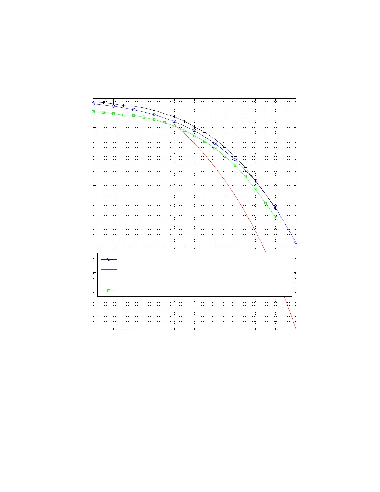
1 Linear -Programming Decoding of Nonbinary Linear Cod es Mark F . Flanagan, Member , IEEE, V italy Skachek, Member , IEEE, Eimear Byrne, and Marcus Greferath Abstract A framework for linear-program ming (LP) decoding of n onbina ry linear code s over rin gs is de- veloped. This f ramework f acilitates linear-progra mming based reception for coded mo dulation systems which use direct mo dulation mapping of coded symbols. It is pr oved that the resultin g L P decod er has the ‘maximu m-likelihood certificate’ property . It is a lso shown that the decoder output is th e lo west cost pseudoco dew ord. Equiv ale nce between pseu docod ew ords of the lin ear pro gram and p seudoco dew ords of graph covers is proved. It is also proved that if th e m odulator-chann el com bination satisfies a particu lar symmetry conditio n, the codeword err or rate per forman ce is in depend ent o f the transmitted c odeword. T wo alternative p olytopes for use with lin ear-programmin g decoding are studied, a nd it is shown th at for many classes of codes these poly topes yield a c omplexity advantage for de coding. Th ese p olytope representatio ns lead to polyno mial-time decoders for a wide variety of classical non binary linear c odes. LP decoding perfor mance is illustrated for the [11 , 6] ter nary Golay co de with ternary PSK modulatio n over A WGN, and in this case it is shown that the perfo rmance o f the LP deco der is comparab le to codeword-error-rate-optim um hard-d ecision based decoding . LP decoding is also simulated for mediu m- length te rnary and quater nary LDPC co des with corre sponding PSK mo dulations over A WGN. Keywords: Linear-pro gramming d ecoding , L DPC cod es, pseudo codewords, coded m odulation . This work was supported in part by the Cl aude Shannon Institute for Discrete Mathematics, Coding and Cr yptography (Science Founda tion Ireland Grant 06/MI/006). The material in this paper wa s presented in part at the 7-th International ITG Conference on Source and Channel Coding (SCC), Ulm, Germany , January 2008, and in part at the IEE E International Symposium on Information Theory (ISIT), T oronto , Canada, July 2008. M. F . Flanagan is with the S chool of Electrical, Electronic and Mechanical Engineering, Univ ersit y College Dublin, Belfield, Dublin 4, Ireland (e-mail:mark.flanagan@ieee.or g). V . Skachek, E. Byrne and M. Greferath are w ith the Claude Shannon Institute and the School of Mathematical S ciences, Univ ersity College Dublin, Belfield, Dublin 4, Ireland (e-mail: { vitaly .skachek, ebyrne, marcus.greferath } @ucd.ie). Nov ember 10, 2021 DRAFT I . I N T R O D U C T I O N Low-density parity-chec k (LDPC) codes [1] ha ve become very popular in recent years du e t o their excellent performance under sum-pr odu ct (SP) decoding (or message-passing decoding). The p rimary research focus in this area to date has been on binary LDPC codes. Fini te-length analysis of such LDPC codes under SP decoding is a d iffi cult task. An approach to such an analysis was prop osed in [2] based on t he consid eration of s o-called pseudo codewor ds and their pseudoweights , defined with respect to a structure called the computatio n tr ee . By replacing thi s set of pseudocodewords with another set defined with respect to cover graphs of the T anner graph (here called graph-cover pseudocodewor ds ), the analys is was found to be significantly more tractable while still yielding accurate experimental results [3], [4], [5]. In [6] and [7], the decoding of binary LDPC codes using li near-pr ogramming (LP) decoding was propo sed, and many im portant connectio ns b etween linear-programming decoding and clas- sical message-passin g decoding were establi shed. In particular , i t was shown th at t he LP d ecoder is inhibited by a set o f p seudocodew ords corresponding to points in the LP relaxation polyto pe with rational coordinates (here called linear-pr ogramming pseudo codewor ds ), and that the set of these ps eudocodew ords is equ iv alent to the set of graph-cover pseudocodewords. This represents a m ajor result as it i ndicates that essentially the same phenomenon determi nes performance of LDPC codes under both LP and SP decoding . For high-data-rate comm unication system s, bandwidth-efficient si gnalling schemes are re- quired which necessitate the use of higher-order (nonb inary) modulation. Of course, wit hin such a frame work it is d esirable to use state-of-the-a rt error- correcting codes. Regarding the combi nation of LDPC coding and h igher-order m odulation, bit-int erlea ved coded modu lation (BICM) [8] is a high-performance m ethod which cascades the operations of binary coding, int erlea ving and higher-order constellation mappin g. Here howe ver the problem of system analy sis is exacerbated by the compl ication of joint design of binary code, interleav er and constellatio n mapping; this becomes e ven mo re diffic ult when feedback is in cluded from the decoder to the demodulator [9]. Alternative ly , hi gher -order m odulation may be achieved in conjun ction wit h cod ing by the use o f non binary codes whose symbols m ap d irectly to modul ation signals. A s tudy of such codes over rings, for use wit h PSK modul ation, was performed i n [10], w ith particular focus on the ring of integers modul o 8 . Nonbinary LDPC codes ov er fields ha ve been in vestigated with 2 direct mapping to b inary [11] and nonbinary [12], [13], [14], [15] modulati on si gnals; in all o f this work, SP decoding (with respect to the nonb inary alphabet) was assumed. Rece ntly , some progress has been made on the topic of analysis of such codes; in particular , pseudocodewords of nonbinary codes were defined and some b ounds on the pseudoweights were d eri ved [16]. In this work, w e extend th e approach i n [7] towards coded m odulation, in particul ar to codes over rings mapped to nonbinary m odulation signals. As was don e i n [7 ], we show that the problem of decoding may be form ulated as an LP problem for the nonbi nary case. W e als o show that an appropriate relaxation of the LP leads to a s olution which has the ‘maximum- likelihood (ML) certificate’ property , i.e. if the L P ou tputs a codew ord, then it must be the M L code word. Moreover , we show that if the LP output i s integral, then it must correspond to the ML code word. W e define the graph-cover pseudocodewor ds of the code, and the lin ear- pr ogramming pseudocodewor ds of t he code, and prove t he equiv alence of these two concepts. This shows that the li nks between LP decoding on the relaxation pol ytope and message-passing decoding on t he T anner graph generalize to the n onbinary case. Of course, while we use the term ‘nonbinary’ throughout this paper , our framew ork includes the binary framework as a special case. For coded mod ulation system s usin g maximum -likelihood (ML ) decoding, the concept of geometric uniformit y [17] was introduced as a condit ion which, if satisfied, guarantees codew ord error rate (WER) p erformance i ndependent of t he transm itted codew ord (this condition was used for desi gn of t he coded modu lation systems in [10]). An analogous symmetry condit ion was defined in [18] for binary codes ov er GF (2) with SP decoding; t his was later extended to nonbinary codes over GF ( q ) by i n voking the concept of coset LDPC codes [13], [14]. W e show that for the present frame work, there exists a symmetry condition under which the code word error rate performance is independent of the transm itted code word. This provides a condi tion some what akin to geometric uniform ity for the present framework. It i s notew orthy that th e same symmetry condition has recently been shown to yield codew ord-independent decoder performance in the context of SP decoding [19] and also in the con text of ML decoding [20]. In particular , thi s identifies a ‘natu ral’ mapp ing for n onbinary codes mapped to PSK modulation , w here LP , SP or ML decoding is used with d irect modulation mapping of coded symbols. For the binary framew ork, alternativ e polytope representations were studied which gave a complexity advantage in certain scenarios [6], [7], [21], [22], [23]. Analogous to these works, we define two alternati ve polytope representations, which of fer a smaller n umber of variables 3 and con straints for many classes of non binary codes. W e com pare these representations with the o riginal pol ytope, and show that both o f them have equal error-correcting performance to the original LP relaxatio n. Both of t hese representations lead to polynomial-time decoders for a wide variety of classical nonbinary linear codes. T o dem onstrate performance, LP decoding is simulated for the ternary Golay code m apped to ternary PSK ov er A WGN, and the LP decoder is seen to perform approximately as well as code word-error -rate optim um hard-decision decoding, and approxi mately 1 . 5 dB from t he unio n bound for code word-error -rate optim um soft-decision decoding. The paper is or ganized as follows. Section II introduces general settings and notation. The nonbinary decoding problem is form ulated as a l inear- programming problem in Section III, and basic properties of the d ecoding polytope are studied in Section IV. A suffic ient condit ion for codew ord-independence performance of t he decoder is presented in Section V. Linear- pr ogramming pseudocodewor ds are defined in Section VI , and th eir prop erties are discussed. Their equiv alence to th e graph-cover pseud ocodewor ds i s shown in Section VII . T wo alternativ e polytope representations are presented in Sections VIII and IX, bot h of which hav e equivalent performance to the original b ut may provide l ower -complexity decoding. Simulation results are presented in Section X for some example coded modu lation systems. Finally , some directions for future research are proposed in Section XI. I I . G E N E R A L S E T T I N G S W e consider codes over finite rings (thi s includes codes ove r finite fields, b ut may be more general). Denote by R a ring wi th q elements, by 0 its additive identi ty , and let R − = R \{ 0 } . Let C be a code of length n over t he ring R , defined b y C = { c ∈ R n : c H T = 0 } (1) where H is an m × n m atrix (with ent ries from R ) called the pa rity-chec k ma trix of the code C . Obviously , th e cod e C may admit more than one parity-check matrix ; howe ver we will consider that the parity-check matrix H is fixed i n this paper . Linearity of the code C fol lows di rectly from (1). Also, the rate of the code C is defined as R ( C ) = log q ( |C | ) /n and i s equal to the number of information symbol s per coded symbol. The code C may then be referr ed to as an [ n, log q ( |C | )] linear code ov er R . 4 Denote the set of column ind ices and the set of row indices of H by I = { 1 , 2 , · · · , n } and J = { 1 , 2 , · · · , m } , respectively . W e use notation H j for the j -th row of H , where j ∈ J . Denote by supp ( c ) the support of a vector c . F or each j ∈ J , let I j = supp ( H j ) and d j = |I j | , and let d = max j ∈J { d j } . Giv en any c ∈ R n , we say that parit y-check j ∈ J is satis fied by c if and only if c H T j = X i ∈I j c i · H j,i = 0 . (2) For j ∈ J , define t he single p arity-check code C j over R by C j = { ( b i ) i ∈I j : X i ∈I j b i · H j,i = 0 } Note that while th e symbols of the codewords in C are indexed by I , the sym bols o f the code words i n C j are index ed by I j . W e define the projection mappi ng for parit y-check j ∈ J by x j ( c ) = ( c i ) i ∈I j Then, give n any c ∈ R n , we may say that parity-check j ∈ J is satisfied by c if and only if x j ( c ) ∈ C j , (3) since (2) and (3) are equiv alent. Al so, it i s easil y seen t hat c ∈ C if and only if all parity -checks j ∈ J are satisfied by c . In t his case we say that c is a codewor d of C . W e shall take an example which shall be used to illustrate concepts throughout this paper . Consider the [4 , 2] linear code ov er R = Z 3 with parity-check matrix H =   1 2 2 1 2 0 1 2   (4) Here I 1 = { 1 , 2 , 3 , 4 } , I 2 = { 1 , 3 , 4 } , and the two s ingle parity-check codes C 1 and C 2 , of length d 1 = 4 and d 2 = 3 respectiv ely , are g iv en by C 1 = { ( b 1 b 2 b 3 b 4 ) : b 1 + 2 b 2 + 2 b 3 + b 4 = 0 } and C 2 = { ( b 1 b 3 b 4 ) : 2 b 1 + b 3 + 2 b 4 = 0 } . 5 I I I . D E C O D I N G A S A L I N E A R - P RO G R A M M I N G P RO B L E M Assume that the codew ord ¯ c = ( ¯ c 1 , ¯ c 2 , · · · , ¯ c n ) ∈ C has been transmitted over a q -ary input memoryless channel, and a corrupted word y = ( y 1 , y 2 , · · · , y n ) ∈ Σ n has been recei ved. Here Σ denotes the s et of channel output sym bols; we assume th at th is set eit her has finite cardinali ty , or is equal to R l or C l for some integer l ≥ 1 . In practice, this channel m ay represent the combination of modulato r and physi cal channel. W e assum e hereafter t hat all information words are equally probable, and so all code words are transmitt ed with equal probabil ity . It was s uggested in [6] to represent each sym bol as a bi nary vector of length | R − | , wh ere the entries in the vector are ind icators of a sym bol taking on a particular value. Below , we show how this representation may l ead to a generalization of the framework of [7] to the case of nonbinary coding. This generalization is nontrivial sin ce, while su ch a representation con verts the nonbinary code into a bi nary code, this binary code is not l inear and therefore the analysis in [6], [7] is not directly app licable. For use in the following deriv ation, we s hall define the mapping ξ : R − → { 0 , 1 } q − 1 ⊂ R q − 1 , by ξ ( α ) = x = ( x ( γ ) ) γ ∈ R − , such that, for each γ ∈ R − , x ( γ ) =    1 if γ = α 0 otherwise. W e note that the m apping ξ is one-to-one, and its im age i s the set of binary vectors of lengt h q − 1 wi th Hamming weight 0 o r 1. Building on this, we also d efine Ξ : R n − → { 0 , 1 } ( q − 1) n ⊂ R ( q − 1) n , according to Ξ ( c ) = ( ξ ( c 1 ) | ξ ( c 2 ) | · · · | ξ ( c n )) . W e note that Ξ is also one-to-one. Now , for vectors f ∈ R ( q − 1) n , we adopt the notation f = ( f 1 | f 2 | · · · | f n ) , 6 where ∀ i ∈ I , f i = ( f ( α ) i ) α ∈ R − . Also, we may use this notation to write the inv erse of Ξ as Ξ − 1 ( f ) = ( ξ − 1 ( f 1 ) , ξ − 1 ( f 2 ) , · · · , ξ − 1 ( f n )) . W e also define a function λ : Σ − → ( R ∪ {±∞} ) q − 1 by λ = ( λ ( α ) ) α ∈ R − , where, for each y ∈ Σ , α ∈ R − , λ ( α ) ( y ) = log  p ( y | 0) p ( y | α )  , and p ( y | c ) denotes the channel output probability (density) conditioned on the channel input . W e extend t his to a m ap on Σ n by defining Λ ( y ) = ( λ ( y 1 ) | λ ( y 2 ) | . . . | λ ( y n )) . The codew ord-error -rate-optimum recei ver operates according to t he maximum a pos teriori (MAP) decision rule: ˆ c = arg max c ∈C p ( c | y ) = arg max c ∈C p ( y | c ) p ( c ) p ( y ) . Here p ( · ) denotes p robability i f Σ has finite cardinality , and probabilit y dens ity if Σ has i nfinite cardinality . By assumption , th e a priori probabi lity p ( c ) i s uniform over codewords, and p ( y ) i s indepen- dent of c . Therefore, the d ecision rule reduces to maximum-li kelihood (ML) decoding: ˆ c = arg max c ∈C p ( y | c ) = arg max c ∈C n Y i =1 p ( y i | c i ) = arg max c ∈C n X i =1 log( p ( y i | c i )) = arg min c ∈C n X i =1 log  p ( y i | 0) p ( y i | c i )  = arg min c ∈C n X i =1 λ ( y i ) ξ ( c i ) T = arg min c ∈C Λ ( y ) Ξ ( c ) T , 7 where we have made use of th e mem oryless prop erty of the channel, and of t he fact that i f c i = α ∈ R − , then λ ( y i ) ξ ( c i ) T = λ ( α ) ( y i ) . This is then equi va lent t o ˆ c = Ξ − 1 ( ˆ f ) where ˆ f = arg min f ∈K ( C ) Λ ( y ) f T , (5) and K ( C ) represents the con vex hu ll of all p oints f ∈ R ( q − 1) n which correspond to code words, i.e. K ( C ) = H con v  Ξ ( c ) : c ∈ C  . Therefore it i s seen that th e M L decoding prob lem reduces to the mi nimization o f a li near objective function (or cost functio n) over a polyto pe in R ( q − 1) n . The number of variables and constraints for this linear program is exponential in n , and it is therefore too complex for practical implementati on. T o circumvent this problem, we formulate a relaxed LP problem, as shown next. The solution we s eek for f (i. e. the desired LP output) is f = Ξ ( ¯ c ) = ( ξ ( ¯ c 1 ) | ξ ( ¯ c 2 ) | . . . | ξ ( ¯ c n )) . (6) Note t hat (6) implies that the solut ion we seek for each f i ( i ∈ I ) is an indicator function which “points” to the i -th transmitted symbol ¯ c i , i.e. ∀ i ∈ I : f ( α ) i =    1 if α = ¯ c i 0 otherwise. W e now introduce auxili ary va riables whose const raints, along wi th t hose of t he elements of f , will form the relaxed LP problem. W e denote these auxiliary variables by w j, b for j ∈ J , b ∈ C j , and we denote the vector containing these variables as w =  w j  j ∈J where w j =  w j, b  b ∈C j ∀ j ∈ J . The solution we seek for these variables is ∀ j ∈ J : w j, b =    1 if b = x j ( ¯ c ) 0 otherwise. (7) 8 Note that th e soluti on we seek for each w j ( j ∈ J ) is an indi cator function which “point s” to the j -th transmitted l ocal code word x j ( ¯ c ) . Based on (7), we impose the con straints ∀ j ∈ J , ∀ b ∈ C j , w j, b ≥ 0 , (8) and ∀ j ∈ J , X b ∈C j w j, b = 1 . (9) Finally , we note that t he solution we seek (giv en by the combination of (6) and (7)) satisfies the further constraints ∀ j ∈ J , ∀ i ∈ I j , ∀ α ∈ R − , f ( α ) i = P b ∈C j , b i = α w j, b . (10) It is interesting to note that from (8) and (9), each vector w j (for j ∈ J ) may be i nterpreted as a probability distribution for the local codew o rd b ∈ C j , in which case each f i (for i ∈ I ) has a natural interpretation (via (10)) as the correspond ing probabi lity distri bution for the i -th coded symbol c i ∈ R . The following example illustrates th e connection (10) between f and w . Example 3.1: Consider the example [4 , 2] code over Z 3 defined by th e parity-check ma- trix (4). The second row H 2 of the p arity-check matrix corresponds to the parit y-check equation 2 b 1 + b 3 + 2 b 4 = 0 over Z 3 . H ere b = ( b 1 b 3 b 4 ) ∈ C 2 . Assum e that the values o f w 2 , b for b ∈ C 2 are as giv en in the following table. b 1 b 3 b 4 w 2 , b b 1 b 3 b 4 w 2 , b b 1 b 3 b 4 w 2 , b 000 0 . 01 102 0 . 05 201 0 . 15 011 0 . 04 110 0 . 07 212 0 . 32 022 0 . 05 121 0 . 08 220 0 . 23 Then, some of the v alues of f ( α ) i are as follows: f (2) 1 = 0 . 15 + 0 . 32 + 0 . 2 3 = 0 . 7 ; f (1) 2 = 0 . 04 + 0 . 07 + 0 . 3 2 = 0 . 43 ; f (2) 3 = 0 . 05 + 0 . 05 + 0 . 3 2 = 0 . 42 . 9 Constraints (8)-(10) may be interpreted as the statement that for all j ∈ J , the vector ˆ f j = ( f i ) i ∈I j lies in the con vex hull K ( C j ) . Cons traints (8)-(10) form a polyto pe which we denote by Q . The m inimization of th e obj ectiv e function (5) ove r Q forms the relaxed LP decoding problem. This LP is defined by O ( q n + q d m ) v ariables and O ( q n + q d m ) constraints, and therefore, the number of va riables and of cons traints scales as approximately q d . W e note that the further constraints ∀ j ∈ J , ∀ b ∈ C j , w j, b ≤ 1 , (11) ∀ i ∈ I , ∀ α ∈ R − , 0 ≤ f ( α ) i ≤ 1 . (12) and ∀ i ∈ I , X α ∈ R − f ( α ) i ≤ 1 . (13) follow from the constraints (8)-(10), for any ( f , w ) ∈ Q . Now we may define the decoding algorithm, which works as foll ows. The decoder solves the LP problem of minimizi ng the objective function (5) subj ect to t he constraints (8)-(10). If f ∈ { 0 , 1 } ( q − 1) n , the o utput is the codeword Ξ − 1 ( f ) (we shall p rove i n the n ext section that this ou tput i s i ndeed a codeword). This code word may then be the correct one (we call this ‘correct decoding’) or an i ncorrect one (we call t his ‘in correct decoding’). If f / ∈ { 0 , 1 } ( q − 1) n , the decoder reports a ‘decoding failure’. Note t hat in this paper , we say that the decoder makes a cod ewor d err or when t he decoder output is no t equal to the transmitt ed codeword (th is coul d correspond to a ‘decoding f ailure’, or to an ‘incorrect decoding’). The tim e complexity of an LP so lver depends on the n umber of v ariables and constraints in the LP problem. The s implex met hod is a popul ar and practically effic ient algorithm for so lving LP problems. Howe ver , its worst-case time complexity has been shown to be exponential in the number of variables. There are other kno wn LP solvers, such as solvers that are based on interior-point method s [24, Chapter 11], which ha ve tim e complexity poly nomial in the number of variables and constraints. For more detail the reader may also refer to [25]. W e note, howe ver , that the standard iterative decoding algorith ms (such as the m in-sum or sum -product algorithms) hav e time complexity which is linear i n th e block length of the code, and therefore significantly outperform the LP decoder in t erms of ef ficiency . 10 I V . P O L Y T O P E P R O P E R T I E S The analysis in this sectio n is a direct generalization of the results in [7]. Definition 4.1: An int e gral po int in a polyto pe is a poin t wit h all inte ger coordinates. Pr opos ition 4.1: 1) Let ( f , w ) ∈ Q , and f ( α ) i ∈ { 0 , 1 } for e very i ∈ I , α ∈ R − . Then Ξ − 1 ( f ) ∈ C . 2) Con versely , for every codeword c ∈ C , there e xists w such that ( f , w ) is an integral p oint in Q with f = Ξ ( c ) . Pr oof : 1) Suppose ( f , w ) ∈ Q , and f ( α ) i ∈ { 0 , 1 } for e very i ∈ I , α ∈ R − . Let c = Ξ − 1 ( f ) ; by (13), this is well defined. Now , fix some j ∈ J and define t = x j ( c ) . Note that from these definitions it follows that for any i ∈ I , α ∈ R − , f ( α ) i = 1 if and only if t i = α . Now let r ∈ C j , r 6 = t . Sin ce r and t are distinct, there must exist α ∈ R − and l ∈ I j such that either r l = α and t l 6 = α , or t l = α and r l 6 = α . W e exa mine these two cases separately . • If r l = α and t l 6 = α , then by (10) f ( α ) l = 0 = X b ∈C j , b l = α w j, b . Therefore w j, b = 0 for all b ∈ C j with b l = α , and in particular w j, r = 0 . • If t l = α and r l 6 = α , then by (9) and (10) 0 = 1 − f ( α ) l = X b ∈C j w j, b − X b ∈C j , b l = α w j, b = X b ∈C j , b l 6 = α w j, b . Therefore w j, b = 0 for all b ∈ C j with b l 6 = α , and in particular w j, r = 0 . It follows t hat w j, r = 0 for all r ∈ C j , r 6 = t . But b y (9) thi s implies that t ∈ C j (and that w j, t = 1 ). Applying this ar gument for e very j ∈ J i mplies c ∈ C . 2) For c ∈ C , we l et f = Ξ ( c ) . For each parity-check j ∈ J , we let t = x j ( c ) ∈ C j and then set ∀ j ∈ J : w j, b =    1 if b = t 0 otherwise. 11 It is easily checked that the resulti ng point ( f , w ) is integral and satisfies const raints (8)- (10). The follo wing proposition assures the so -called ML certificate property . Pr opos ition 4.2: Suppose that the decoder output s a codew ord c ∈ C . Then, c is t he maximum-li kelihood codeword. The proof of thi s proposition is straigh tforward. Th e reader can refer to a simil ar proof for the binary case in [7]. V . C O D E WO R D - I N D E P E N D E N T D E C O D E R P E R F O R M A N C E In t his section, we state and prov e a theorem on decoder performance, namely , that under a certain symm etry condition , the probability of code word error is in dependent of t he transmi tted code word. The proof generalizes the corresponding proo f for the binary case which may be found in [6], [7]. Symmetry Condition. For each β ∈ R , there exists a bijection τ β : Σ − → Σ , such that the channel output probability (density) conditioned on t he channel input satisfies p ( y | α ) = p ( τ β ( y ) | α − β ) , (14) ∀ y ∈ Σ , α ∈ R . When Σ i s equal to R l or C l for l ≥ 1 , the mapping τ β is assum ed to be isometric with respect to Euclidean d istance in Σ , for e very β ∈ R . Note that the sym metry condi tion above is very similar to that introduced in [20] which guarantees code word-independent performance under ML decodi ng. Theor em 5. 1: Under the stated symmet ry condi tion, the probability of codew ord error is independent of the transmitted cod e word. Pr oof : W e shall p rove t he theorem for th e case where Σ has infinit e cardinality; the case of discrete Σ may be handled similarly . Fix some codew ord c ∈ C , c 6 = 0 . W e wi sh to p rove that Pr ( Err | c ) = Pr ( Err | 0 ) , 12 where Pr ( Err | c ) denot es the probabi lity of codeword error g iv en th at the codeword c was transmitted. Now Pr ( Err | c ) = Pr ( y ∈ B ( c ) | c ) , where B ( c ) = { y ∈ Σ n : ∃ ( f , w ) ∈ Q , f 6 = Ξ ( c ) with Λ ( y ) f T ≤ Λ ( y ) Ξ ( c ) T } . Here B ( c ) is the set of all receive d words which may cause code word error , given th at c was transmitted. Recall that the elements of Λ ( y ) are given by λ ( α ) ( y i ) = log  p ( y i | 0) p ( y i | α )  , (15) for i ∈ I , α ∈ R − . Also Pr ( Err | 0 ) = Pr ( y ∈ B ( 0 ) | 0 ) where B ( 0 ) = { ˜ y ∈ Σ n : ∃ ( ˜ f , ˜ w ) ∈ Q , ˜ f 6 = Ξ ( 0 ) with Λ ( ˜ y ) ˜ f T ≤ Λ ( ˜ y ) Ξ ( 0 ) T } . So we write Pr ( Err | c ) = Z y ∈ B ( c ) p ( y | c ) d y (16) and Pr ( Err | 0 ) = Z ˜ y ∈ B ( 0 ) p ( ˜ y | 0 ) d ˜ y . (17) Now , setting α = β in the symmetry condition (14) yields p ( y | β ) = p ( τ β ( y ) | 0) (18) for any y ∈ Σ , β ∈ R . W e now define G : Σ n − → Σ n and ˜ y as follows. ˜ y = G ( y ) s.t. ∀ i ∈ I : ˜ y i = τ β ( y i ) where β = c i . W e note that G is a bijection from the s et Σ n to itself, and that if y , z ∈ Σ n and β = c i then k y i − z i k 2 = k τ β ( y i ) − τ β ( z i ) k 2 13 and so k G ( y ) − G ( z ) k 2 = k y − z k 2 i.e. G is isometric with respect to Eu clidean distance in Σ n . W e prove that the integral (16) may be transformed to (17) vi a the substi tution ˜ y = G ( y ) . First, we hav e p ( y | c ) = Y i ∈I p ( y i | c i ) = Y β ∈ R Y i ∈I ,c i = β p ( y i | β ) = Y β ∈ R Y i ∈I ,c i = β p ( τ β ( y i ) | 0) = Y β ∈ R Y i ∈I ,c i = β p ( ˜ y i | 0) = Y i ∈I p ( ˜ y i | 0) = p ( ˜ y | 0 ) . Since G is i sometric with respect to Eu clidean distance i n Σ n , it foll ows that the Jacobian determinant o f the trans formation i s equal to unity . Therefore, to complete the proof, we need only show that y ∈ B ( c ) if and only if ˜ y ∈ B ( 0 ) . W e begin by relatin g the elements of Λ ( y ) to th e elements of Λ ( ˜ y ) . Let i ∈ I , α ∈ R − . Suppose c i = β ∈ R . W e then hav e λ ( α ) ( y i ) = log  p ( y i | 0) p ( y i | α )  = log  p ( τ β ( y i ) | − β ) p ( τ β ( y i ) | α − β )  = log  p ( ˜ y i | − β ) p ( ˜ y i | α − β )  . This yields λ ( α ) ( y i ) =          λ ( α ) ( ˜ y i ) if β = 0 − λ ( − α ) ( ˜ y i ) if α = β λ ( α − β ) ( ˜ y i ) − λ ( − β ) ( ˜ y i ) otherwise. 14 Next, for any po int ( f , w ) ∈ Q we define a new poi nt ( ˜ f , ˜ w ) as follo ws. For β = c i and all i ∈ I , α ∈ R − , ˜ f ( α ) i =    1 − P γ ∈ R − f ( γ ) i if α = − β f ( α + β ) i otherwise. (19) For all j ∈ J , r ∈ C j we define ˜ w j, r = w j, b where b = r + x j ( c ) . Next we prove that for every ( f , w ) ∈ Q , the new point ( ˜ f , ˜ w ) lies in Q and thus is a feasible solutio n for th e L P . Const raints (8) and (9) obviousl y hold from the definition of ˜ w . T o verify (10), we let j ∈ J , i ∈ I j and α ∈ R − . W e also let β = c i . W e now check two cases: • If α = − β , ˜ f ( α ) i = 1 − X γ ∈ R − f ( γ ) i = X b ∈C j w j, b − X γ ∈ R − X b ∈C j , b i = γ w j, b = X b ∈C j , b i =0 w j, b = X r ∈C j , r i = α ˜ w j, r . • If α 6 = − β , ˜ f ( α ) i = f ( α + β ) i = X b ∈C j , b i = α + β w j, b = X r ∈C j , r i = α ˜ w j, r . Therefore ( ˜ f , ˜ w ) ∈ Q , i.e. ( ˜ f , ˜ w ) is a feasible solution for the LP . W e wri te ( ˜ f , ˜ w ) = L ( f , w ) . W e als o note t hat the m apping L is a bijectio n from Q t o itself; thi s is easily shown by verifying the in verse f ( α ) i =    1 − P γ ∈ R − ˜ f ( γ ) i if α = β ˜ f ( α − β ) i otherwise (20) 15 for all i ∈ I , α ∈ R − , and w j, b = ˜ w j, r where r = b − x j ( c ) for all j ∈ J , b ∈ C j . W e now prove that for ev ery ( f , w ) ∈ Q , ( ˜ f , ˜ w ) = L ( f , w ) s atisfies Λ ( y ) f T − Λ ( y ) Ξ ( c ) T = Λ ( ˜ y ) ˜ f T − Λ ( ˜ y ) Ξ ( 0 ) T . (21) W e achiev e th is by proving λ ( y i ) f T i − λ ( y i ) ξ ( c i ) T = λ ( ˜ y i ) ˜ f T i − λ ( ˜ y i ) ξ (0) T (22) for ever y i ∈ I . W e may th en obtain (21) by sum ming (22) over i ∈ I . Let β = c i . W e consider two cases: • If β = 0 , (22) becomes λ ( y i ) f T i = λ ( ˜ y i ) ˜ f T i which holds since λ ( α ) ( ˜ y i ) = λ ( α ) ( y i ) and ˜ f ( α ) i = f ( α ) i for all α ∈ R − in this case. • If β 6 = 0 , λ ( y i ) f T i − λ ( y i ) ξ ( c i ) T = X γ ∈ R − λ ( γ ) ( y i ) f ( γ ) i − λ ( β ) ( y i ) = X γ ∈ R − γ 6 = β  λ ( γ − β ) ( ˜ y i ) − λ ( − β ) ( ˜ y i )  f ( γ ) i − λ ( − β ) ( ˜ y i ) f ( β ) i + λ ( − β ) ( ˜ y i ) = X α ∈ R − α 6 = − β λ ( α ) ( ˜ y i ) f ( α + β ) i + λ ( − β ) ( ˜ y i )   1 − X γ ∈ R − f ( γ ) i   = X α ∈ R − λ ( α ) ( ˜ y i ) ˜ f ( α ) i = λ ( ˜ y i ) ˜ f T i − λ ( ˜ y i ) ξ (0) T where we have made use of the substitutio n α = γ − β i n the thi rd line. Therefore (22) holds, proving (21). 16 Finally , we note that i t i s easy to show , using (19) and (20), that f = Ξ ( c ) if and only if ˜ f = Ξ ( 0 ) . Putt ing toget her these results, we may make the following statement. Suppose we are given y , ˜ y ∈ Σ n with ˜ y = G ( y ) . Then the point ( f , w ) ∈ Q satisfies f 6 = Ξ ( c ) and Λ ( y ) f T ≤ Λ ( y ) Ξ ( c ) T if and only if t he point ( ˜ f , ˜ w ) = L ( f , w ) ∈ Q s atisfies ˜ f 6 = Ξ ( 0 ) and Λ ( ˜ y ) ˜ f T ≤ Λ ( ˜ y ) Ξ ( 0 ) T . Th is statement, along wi th the fact that both G and L are bijective, proves th at y ∈ B ( c ) if and only if ˜ y ∈ B ( 0 ) . W e next provide, with details, some examples of modulator-channel com binations for which the symmetry conditions hold. Example 5.1: Discr ete memoryless q -ary symmetri c channel. Here we denote the ring el- ements by R = { a 0 , a 1 , · · · , a q − 1 } . Also Σ = { s 0 , s 1 , · · · , s q − 1 } , where t he channel o utput probability conditioned on the channel i nput satisfies, for each t, k ∈ { 0 , 1 , · · · , q − 1 } , p ( s t | a k ) =    (1 − p ) if t = k p/ ( q − 1) otherwise , where p represents the probabil ity of transmission error . Here we may define the mapping τ β for each β ∈ R according to τ β ( s t ) = s ℓ where a ℓ = a t − β for all t ∈ { 0 , 1 , · · · q − 1 } . It i s easy to check that t hese mappings are bijectiv e and satis fy the symmetry condition. Example 5.2: Orthogonal mo dulation over A WGN. Here Σ = R q , and denoting the ring elements by R = { a 0 , a 1 , · · · , a q − 1 } , the m odulation m apping may be written withou t loss of generality as M : R − → R q , such that, for each k = 0 , 1 , · · · , q − 1 , M ( a k ) = x = ( x (0) , x (1) , · · · , x ( q − 1) ) , where x ( t ) =    1 if t = k 0 otherwise. 17 Here we may defi ne the mapping τ β for e ach β ∈ R according to (where y = ( y (0) , y (1) , · · · , y ( q − 1) ) ∈ R q , z = ( z (0) , z (1) , · · · , z ( q − 1) ) ∈ R q ) τ β ( y ) = z such that for each l ∈ { 0 , 1 , · · · , q − 1 } , z ( ℓ ) = y ( k ) where a k = a l + β . It is easily checked that these mappi ngs are bij ectiv e and isometric, and sati sfy the symm etry condition. Example 5.3: q -ary P SK modulation over A WGN. Here Σ = C , and again denoting the rin g elements by R = { a 0 , a 1 , · · · , a q − 1 } , the m odulation mapping may be written without l oss of generality as M : R 7→ C such that M ( a k ) = exp  ı 2 π k q  (23) for k = 0 , 1 , · · · , q − 1 (here ı = √ − 1 ). Here (18), together wi th th e rotational symmetry of the q -ary PSK constell ation, motiv ates us to define, for ev ery β = a k ∈ R , τ β ( x ) = exp  − ı 2 π k q  · x ∀ x ∈ C (24) Next, we also imp ose t he conditi on t hat R under addition is a cyclic g roup. T o s ee why we impose this condition, let α = a k ∈ R and β = a l ∈ R . By t he symmetry condition we must hav e p ( y i | α + β ) = p ( τ α + β ( y i ) | 0) and also p ( y i | α + β ) = p ( τ β ( y i ) | α ) = p ( τ α ( τ β ( y i )) | 0) . In order to equate these two expressions, we impose th e condition τ α + β ( x ) = τ α ( τ β ( x )) for all x ∈ C , α, β ∈ R . Letting α + β = a p ∈ R , and using (24) yields exp  − ı 2 π k q  · exp  − ı 2 π l q  = exp  − ı 2 π p q  18 and thus p ≡ ( k + l ) mod q . Therefore, we must ha ve a k + a l = a ( k + l ) mod q (25) for all a k , a l ∈ R . This implies that R , under addition, i s a cyclic group. It is easy to check that the condition that R u nder addition is cyclic, encapsulated by (25), along with the modulati on mapping (23), satisfies the symm etry condi tion, w here the appropriate mappings τ β are give n by (24). This means t hat code word-independent pe rformance is guaranteed for such systems using nonbi nary cod es with PSK m odulation. This appl ies to A WGN, flat fading wireless channels, and OFDM systems transm itting over frequency selective channels with suffi ciently long cyclic prefix. V I . L I N E A R P RO G R A M M I N G P S E U D O C O D E W O R D S Definition 6.1: A linear-pr ogramming pseudocodewor d (LP pseudocod e word) of the code C , with parity-check matrix H , is a pair ( h , z ) where h ∈ R ( q − 1) n and z =  z j, b  j ∈J , b ∈C j , where z j, b is a nonnegati ve integer for all j ∈ J , b ∈ C j , such that th e following con straints are satisfied: ∀ j ∈ J , ∀ i ∈ I j , ∀ α ∈ R − , h ( α ) i = P b ∈C j , b i = α z j, b , (26) and ∀ j ∈ J , X b ∈C j z j, b = M , (27) where M is a nonnegativ e integer i ndependent of j . It follows from (26) that h ( α ) i is a nonnegati ve i nteger for all i ∈ I , α ∈ R − . W e note that t he further constraints ∀ j ∈ J , ∀ b ∈ C j , z j, b ≤ M , (28) ∀ i ∈ I , ∀ α ∈ R − , 0 ≤ h ( α ) i ≤ M , (29) 19 and ∀ i ∈ I , X α ∈ R − h ( α ) i ≤ M , (30) follow from the constraints (26) and (27). For each i ∈ I , we also define h (0) i = M − X α ∈ R − h ( α ) i . (31) By (30), h (0) i is a nonnegativ e integer for all i ∈ I . Now , for any j ∈ J , i ∈ I j we ha ve h (0) i = M − X α ∈ R − h ( α ) i = X b ∈C j z j, b − X α ∈ R − X b ∈C j ,b i = α z j, b = X b ∈C j ,b i =0 z j, b where we ha ve u sed (26) and (27). Corresponding to the LP pseudocodeword ( h , z ) defined above, we define the n ormalized LP pseudocodewor d as the vector obtained by scaling of ( h , z ) by a factor 1 / M . W e also define the n × q LP pseud ocodewor d matrix H =  h ( α ) i  i ∈I ; α ∈ R . The normalized LP pseudocodewor d matrix is defined as (1 / M ) · H . Note that if we interpret { z j, b / M } (for each j ∈ J ) as a probability distri bution for the local code word b ∈ C j , then th e i -th row of the normali zed LP pseudocodeword matrix (for i ∈ I ) can be in terpreted as the corresponding probabil ity distribution for the i -th coded symbol c i ∈ R . This i dea of interpretating pseudocodewords as probability distributions was used in [3] for the binary case. Example 6.1: As an illustratio n, we provide an LP pseudocodew ord for the example [4 , 2] code over Z 3 defined by the parity-check matrix (4). The reader may check that ( h (1) 1 , h (1) 2 , h (1) 3 , h (1) 4 ) = (2 2 2 2) (32) and ( h (2) 1 , h (2) 2 , h (2) 3 , h (2) 4 ) = (2 2 0 0) (33) 20 together with z 1 , b =          2 if b = (2 1 1 0) 2 if b = (1 2 0 1) 0 otherwise, (34) and z 2 , b =          2 if b = (2 0 1) 2 if b = (1 1 0) 0 otherwise, (35) satisfy (26) and (27), where M = 4 in (27). W e also obtain from (31) ( h (0) 1 , h (0) 2 , h (0) 3 , h (0) 4 ) = (0 0 2 2) . Therefore (32)-(35) define an LP pseudocode word, with pseudocodeword matrix H =        0 2 2 0 2 2 2 2 0 2 2 0        . (36) The corresponding normalized LP pseudocodew ord matrix is then given by 1 4 · H =        0 1 2 1 2 0 1 2 1 2 1 2 1 2 0 1 2 1 2 0        . (37) Here the prob abilistic interpretation of t his no rmalized LP pseudocode word matrix corresponds to an equiprobable dist ribution of sym bols from { 1 , 2 } for the first two symbol s in the codeword, and an equiprobable distrib ution of sym bols fr om { 0 , 1 } for the last two symbols in the code word. Theor em 6. 1: Assume that the all-zero code word was transmitt ed. 1) If t he LP decoder m akes a code word error , then there exists some LP pseud ocodew o rd ( h , z ) , h 6 = 0 , such that Λ ( y ) h T ≤ 0 . 2) If there exists som e LP pseudocodew ord ( h , z ) , h 6 = 0 , such that Λ ( y ) h T < 0 , then the LP decoder makes a codeword error . Pr oof : Th e proof follo ws th e lines of its counterpart in [7]. 21 1) Let ( f , w ) b e the p oint in Q which minimizes Λ ( y ) f T . Suppose there is a codew ord error; then f 6 = 0 , and we must hav e Λ ( y ) f T ≤ 0 . Next, we construct the LP pseudocodeword ( h , z ) as follows. Sin ce the LP has ration al coef ficients, all elements of the vectors f and w must be rational. Let M denote their lowest common denomin ator; si nce f 6 = 0 we may have M > 0 . Now set h ( α ) i = M · f ( α ) i for all i ∈ I , α ∈ R − and set z j, b = M · w j, b for all j ∈ J and b ∈ C j . By (8)-(10), ( h , z ) is an LP pseudocodew ord and h 6 = 0 since f 6 = 0 . Also Λ ( y ) f T ≤ 0 implies Λ ( y ) h T ≤ 0 . 2) Now , supp ose that an LP ps eudocodew ord ( h , z ) with h 6 = 0 satis fies Λ ( y ) h T < 0 . Since h 6 = 0 we have M > 0 in (27). No w , set f ( α ) i = h ( α ) i / M for all i ∈ I , α ∈ R − , and set w j, b = z j, b / M for all j ∈ J and b ∈ C j . It i s straightforward to check t hat ( f , w ) satisfies all the constraints of the polyt ope Q . Al so, h 6 = 0 impl ies f 6 = 0 . Fin ally , Λ ( y ) h T < 0 implies Λ ( y ) f T < 0 . Therefore, the LP decoder will make a codeword error . V I I . E Q U I V A L E N C E B E T W E E N P S E U D O C O D E W O R D C O N C E P T S A. T anner Graphs and Graph-Co ver Ps eudocodewor ds The T anner graph o f a linear cod e C over R is an equiv al ent character ization o f the code’ s parity-check matrix H . The T anner graph G = ( V , E ) has verte x set V = { u 1 , u 2 , · · · , u n } ∪ { v 1 , v 2 , · · · , v m } , and there is an edge betw een u i and v j if and only if H j,i 6 = 0 . This edge is labelled with the v alue H j,i . W e denote by N ( v ) the set of neighbors of a vertex v ∈ V . For any word c = ( c 1 , c 2 , · · · , c n ) ∈ R n , t he T anner graph allows an equiv alent graphical statement of the condi tion c ∈ C j for each j ∈ J , as follows. The variable vertex u i is labelled with t he value c i for each i ∈ I . Equation (2) (or (3)) is then equiv alent to the conditio n that for vertex v j , the sum, over all vertices in N ( v j ) , of the vertex labels multipl ied by the corresponding edge labels is zero. This graphical m eans of checking whether a parity-check i s satisfied by c ∈ R n will be u seful when defining graph-cove r p seudocodew ords later in th is section. T o illustrate this concept, Figure 1 s hows the T anner graph for the codeword c = (1 0 2 1) of the example [4 , 2] code over Z 3 defined by the parity-check matrix (4). In Figure 1, edge labels are s hown in square brackets, and vertex labels in round brackets. The reader m ay check that for 22 u 1 (1) u 2 (0) u 3 (2) u 4 (1) v 1 v 2 [1] [2] [2] [1] [2] [1] [2] Fig. 1. T anner grap h for the example [4 , 2] code o ver Z 3 . Edge labels are sho wn in square brackets, and v ertex l abels in round bracke ts. For each parity-check j , t he sum, ove r all vertices in N ( v j ) , of the v ertex l abels multiplied by the corresponding edge labels is zero; t herefore all parity-checks are satisfied. each parity-check j = 1 , 2 , the su m, ov er all vertices in N ( v j ) , of the verte x labels multi plied by the corresponding edge labels is zero. W e next d efine what is meant by a finit e cov er o f a T anner graph. Definition 7.1: ([4]) A graph ˜ G = ( ˜ V , ˜ E ) is a finite cover of the T anner graph G = ( V , E ) if there exists a m apping Π : ˜ V − → V which i s a graph homom orphism ( Π takes adjacent vertices of ˜ G to adjacent vertices of G ), such that for e very vertex v ∈ G and every ˜ v ∈ Π − 1 ( v ) , the neighborhood N ( ˜ v ) o f ˜ v (including edge labels) is mapped b ijective ly t o N ( v ) . Definition 7.2: ([4]) A cover of the graph G is said to hav e degree M , where M is a positive integer , i f | Π − 1 ( v ) | = M for ev ery vertex v ∈ V . W e refer t o such a cover graph as an M -cover of G . Fix som e positive i nteger M . Let ˜ G = ( ˜ V , ˜ E ) be an M -cov er o f the T anner graph G = ( V , E ) representing the code C wi th parity-check matrix H . The vertices in the s et Π − 1 ( u i ) are called copies of u i and are denoted { u i, 1 , u i, 2 , · · · , u i,M } , where i ∈ I . Similarly , the vertices in the set Π − 1 ( v j ) are called copies o f v j and are denoted { v j, 1 , v j, 2 , · · · , v j,M } , where j ∈ J . Less formally , given a cod e C with parity -check matrix H and corresponding T anner graph G , an M -cover of G is a graph who se vertex s et con sists of M copies of u i and M copies of v j , such that for each j ∈ J , i ∈ I j , the M copies of u i and the M copies of v j are connected in an arbitrary one-to-one fashion, wit h edges labell ed by the v alue H j,i . For any M ≥ 1 , a graph-cover pseudocodewor d is a labelling of vertices of th e M -cover 23 graph with values from R such that all p arity-checks are satisfied. W e denote the label o f u i,l by p i,l for each i ∈ I , ℓ = 1 , 2 , · · · , M , and we may then writ e the graph-cov er ps eudocodew ord in vector form as p = ( p 1 , 1 , p 1 , 2 , · · · , p 1 ,M , p 2 , 1 , p 2 , 2 , · · · , p 2 ,M , · · · , p n, 1 , p n, 2 , · · · , p n,M ) . It is easily seen that p belongs to a li near code ˜ C of length M n over R , defined by an M m × M n parity-check matrix ˜ H . T o construct ˜ H , for 1 ≤ i ∗ , j ∗ ≤ M and i ∈ I , j ∈ J , we let i ′ = ( i − 1) M + i ∗ , j ′ = ( j − 1 ) M + j ∗ , and so ˜ H j ′ ,i ′ =    H j,i if u i,i ∗ ∈ N ( v j,j ∗ ) 0 otherwise . It may be seen that ˜ G is the T anner graph of the code ˜ C correspond ing to the parity-check matrix ˜ H . W e also define the n × q graph-cover pseudocodewor d matrix P =  m ( α ) i  i ∈I ; α ∈ R , where m ( α ) i = |{ ℓ ∈ { 1 , 2 , · · · , M } : p i,ℓ = α }| ≥ 0 , for i ∈ I , α ∈ R , i.e. m ( α ) i is equal to the number of copies of u i which are labelled with α , for each i ∈ I , α ∈ R . The norma lized graph-cover pseudocodewor d matrix is defined as (1 / M ) · P . This matrix representatio n is sim ilar t o th at defined in [16]. Note that the i -th row of the normali zed graph-cov er pseudocodeword m atrix (for i ∈ I ) can be v iewe d as a probability distribution for the i -th coded symbol c i ∈ R , in a simi lar manner to the case of the normali zed LP pseudocodew ord matrix. Another representation, which we shall us e in Section IX, is the graph-cover pseudocodewor d vector m = ( m i ) i ∈I where m i = ( m ( α ) i ) α ∈ R − for each i ∈ I . Correspondin gly , the norma lized graph-cover pseudocodewor d vector is gi ven by (1 / M ) · m ∈ R ( q − 1) n . It is easily seen t hat for any c ∈ C , th e labell ing of u i,l by the value c i for all i ∈ I , ℓ = 1 , 2 , · · · , M trivially yields a pseudocodeword for all M -covers of G , M ≥ 1 . Howe ver , non-trivial pseudocodewords exist i n general. 24 Example 7.1: T o ill ustrate these concepts, a graph-cover pseudocodew ord in shown in Figure 2 for the example [4 , 2] code over Z 3 defined by the parity-check matrix (4). Here t he degree of th e cover graph i s M = 4 , and we ha ve p = (1 1 2 2 | 1 1 2 2 | 0 0 1 1 | 0 0 1 1) , and the parity-check matrix of the code ˜ C is gi ven by ˜ H =                    0 0 1 0 2 0 0 0 0 0 2 0 1 0 0 0 0 0 0 1 0 2 0 0 0 0 0 2 0 1 0 0 1 0 0 0 0 0 2 0 2 0 0 0 0 0 1 0 0 1 0 0 0 0 0 2 0 2 0 0 0 0 0 1 0 0 2 0 0 0 0 0 1 0 0 0 0 0 2 0 0 0 0 2 0 0 0 0 0 1 0 0 0 0 0 2 2 0 0 0 0 0 0 0 0 0 1 0 2 0 0 0 0 2 0 0 0 0 0 0 0 0 0 1 0 2 0 0                    Also, the graph-cover pseudocodew ord m atrix corresponding to p i s P =        0 2 2 0 2 2 2 2 0 2 2 0        , (38) and the normalized graph-cov er pseudocode word matrix is 1 4 · P . The graph-cove r pseudocode word vector corresponding to p is m = ( 2 2 | 2 2 | 2 0 | 2 0 ) , and the normalized graph-cov er pseudocode word vector i s 1 4 · m . 25 u 2 , 1 (1) u 2 , 3 (2) u 2 , 4 (2) u 1 , 1 (1) u 1 , 2 (1) u 1 , 4 (2) u 1 , 3 (2) u 2 , 2 (1) u 3 , 1 (0) u 3 , 2 (0) u 3 , 4 (1) u 3 , 3 (1) u 4 , 2 (0) u 4 , 3 (1) u 4 , 4 (1) u 4 , 1 (0) [1] [2] [2] [2] [2] [2] [1] [1] [1] [1] [1] [1] [2] [2] [2] [2] [2] [2] [2] [1] [1] [1] [1] [1] v 1 , 2 v 1 , 3 v 1 , 4 v 2 , 1 v 2 , 2 v 2 , 3 v 2 , 4 v 1 , 1 (2 1 1 0) (1 2 0 1) (1 2 0 1) (2 0 1) (2 0 1) (1 1 0) (1 1 0) [2] (2 1 1 0) [2] [2] [2] Fig. 2. Cover graph of degree 4 and corresponding graph-cove r pseudocode word for the example [4 , 2] code over Z 3 with parity-check matri x given by (4). E dge labels are sho wn in square brackets, and vertex labels in round brackets. T his graph-co ver pseudoco de word corresponds to the LP pseudoco de word described by (32)-(35) via the corresponden ce described in the proof of Theorem 7.1. B. Equ ivalence between LP Pseudocod ewor ds and Graph-Cover Pseudocodewor ds In this section, we sho w the equivalence between the set of LP pseudo code words and the set of graph-cove r pseudocode words. The result is summarized in the following theorem. Theor em 7. 1: Let C be a li near code over th e ring R wit h parity-check matrix H and corre- sponding T anner graph G . Then, t here exists an LP pseudocodeword ( h , z ) with pseudocodeword matrix H if and only i f there exists a graph-cover pseudocodew ord for some M -cover of G with the same pseudocodew ord m atrix. Pr oof : 1) Let ( h , z ) be an LP pseudocodew ord of C , and let G = ( V , E ) be t he T anner graph associated with the parity-check matrix H . W e construct an M -cov er ˜ G = ( ˜ V , ˜ E ) , where M = P b ∈C j z j, b , and corresponding graph-cov er ps eudocodew ord, as foll ows. W e begin with t he vertex set, which consists of M copies of u i , i ∈ I , and M copi es of v j , j ∈ J . 26 Then we proceed as follows: • L abel h ( α ) i copies of u i with the value α , for each i ∈ I , α ∈ R . By (31), all copi es of u i are labelled. • L abel z j, b copies of v j with the v alue b , for every j ∈ J , b ∈ C j . By (27 ), all copies of v j are labelled. • N ext, let T ( α ) i denote the set of copies of u i labelled wit h the value α , for i ∈ I , α ∈ R . Also, for all i ∈ I , j ∈ J , α ∈ R , let R ( α ) i,j denote the set of copies of v j whose label satisfies b i = α . Th e vertices in T ( α ) i and the vertices in R ( α ) i,j are then connected by edges in an arbitrary one-to-one fashion, for e very j ∈ J , i ∈ I j , α ∈ R . All of these edges are labelled wi th the va lue H j,i . First, we note that this is possible because | T ( α ) i | = h ( α ) i = X b ∈C j , b i = α z j, b = | R ( α ) i,j | for e very j ∈ J , i ∈ I j , α ∈ R . Here we hav e used (26)). Second, we note that all checks are satisfied by this labelling. For j ∈ J , consider any copy of v j with label b . By cons truction of t he graph, t he sum, over all vertices in N ( v j ) , of the verte x l abels multiplied b y the corresponding edge labels is X i ∈I j b i · H j,i , which is zero because b ∈ C j . Therefore, this vertex labelling yields a graph-cov er pseudocodew ord of the code C with parity-check matrix H . 2) Now s uppose that there e xists a graph-cov er pseudo codew o rd corresponding to some M - cove r of the T anner graph G of C . Then, • Step 1: for e very i ∈ I , and for ev ery α ∈ R − , w e define h ( α ) i to be the number of copies of u i labelled with the v alue α . • Step 2 : for every copy o f v j , j ∈ J , label the copy with the word b , wh ere b i is equal to the label on the neighbourin g copy of u i , i ∈ I j . Then, for every j ∈ J , b ∈ C j , we define z j, b to be the nu mber of copies of v j labelled with the word b . 27 Step 2 ensures that z j, b are nonnegati ve integers for all j ∈ J and b ∈ C j , and that (27) holds. Al so, to show that (26) hold s, we reason as follows. The right-hand side of (26 ) counts the number of copies o f v j whose labels b satisfy b i = α . By step 2, this is equal to the number of copies of u i labelled with α , which by step 1 is equal to the left-hand side of (26). Therefore, ( h , z ) is an LP pseudocodeword of the code C with parity-check matrix H . As an illustratio n of the correspondences described in this proof, consider the example [4 , 2] code over Z 3 defined by the parity-check m atrix (4). First, note that the LP pseudocodeword of (32)-(35) and the graph-cover pseudocodeword of Figure 2 have the same pseudocodeword matrix, via (36) and (38). Indeed, the reader m ay check that each pseudocodew ord may be deriv ed from the other using the correspondences described in the proof of Theorem 7.1. The next corollary follows im mediately from Theorem 7.1 . Cor ollar y 7 .2: Let C be a linear code over the ring R with parity -check matrix H and corresponding T anner graph G . Then, there exists a (normalized) LP ps eudocodew ord ( h , z ) if and only if there exists a graph-cover pseudocode word for some M -cover of G with (normalized) graph-cove r pseudocode word vector h . Note that this corollary contains two dif ferent equivalence s, one for n ormalized ob jects and the other for non-normalized ones. V I I I . A L T E R NA T I V E P O L Y T O P E R E P R E S E N T A T I O N In this section, we present an alternative polytope for use with linear-programming d ecoding. This polytope may be regarded as a generalizatio n of the “high-density pol ytope” defined in [7]. As we show in this section, the new pol ytope may under some circum stances yi eld a complexity adva ntage over the polytope of Section III. In the s equel, we will analyze the properties of this polytope. First, we introduce some conv enient notation and definitions. Recall that th e rin g R contains q − 1 no n-zero elements; correspondingly , for vectors k ∈ N q − 1 , we adopt the no tation k = ( k α ) α ∈ R − 28 Now , for any j ∈ J , we define t he mapping κ j : C j − → N q − 1 , b 7→ κ j ( b ) defined by ( κ j ( b )) α = |{ i ∈ I j : b i · H j,i = α }| for all α ∈ R − . W e may then characterize the image of κ j , which we denote by T j , as T j = ( k ∈ N q − 1 : X α ∈ R − α · k α = 0 and X α ∈ R − k α ≤ d j ) , for each j ∈ J , where, for any k ∈ N , α ∈ R , α · k =    0 if k = 0 α + · · · + α if k > 0 ( k terms in sum) Note that κ j is n ot a b ijection, in general. W e say th at a local codeword b ∈ C j is k -const rained over C j if κ j ( b ) = k . Next, for any index set Γ ⊆ I , we i ntroduce the fol lowing definitio ns. Let N = | Γ | . W e define the single-parity-check-code, over vectors ind exe d by Γ , by C Γ = ( a = ( a i ) i ∈ Γ ∈ R N : X i ∈ Γ a i = 0 ) . (39) Also define a mapping κ Γ : C Γ − → N q − 1 by ( κ Γ ( a )) α = |{ i ∈ Γ : a i = α }| , and define, for k ∈ T j , C ( k ) Γ = { a ∈ C Γ : κ Γ ( a ) = k } . Belo w , we define a ne w polytope for decoding. Recall that y = ( y 1 , y 2 , · · · , y n ) ∈ Σ n stands for the recei ved (corrupted) word. In the sequel, we m ake use of the foll owing var iables: • For all i ∈ I and all α ∈ R − , we ha ve a variable f ( α ) i . This v ariabl e i s an indicator of the e vent y i = α . • For all j ∈ J and k ∈ T j , we have a variable σ j, k . Similarly to its counterpart in [7], this var iable i ndicates th e contribution to parity-check j of k -constrained local code words ov er C j . 29 • For all j ∈ J , i ∈ I j , k ∈ T j , α ∈ R − , we ha ve a variable z ( α ) i,j, k . This v ariable indicates the portion of f ( α ) i assigned to k -constrained local codew ords over C j . Motiv ated by these variable definitions, for all j ∈ J we impose t he foll owing set of constraints: ∀ i ∈ I j , ∀ α ∈ R − , f ( α ) i = X k ∈T j z ( α ) i,j, k . (40) X k ∈T j σ j, k = 1 . (41) ∀ k ∈ T j , ∀ α ∈ R − , X i ∈I j , β ∈ R − , β H j,i = α z ( β ) i,j, k = k α · σ j, k . (42) ∀ i ∈ I j , ∀ k ∈ T j , ∀ α ∈ R − , z ( α ) i,j, k ≥ 0 . (43) ∀ i ∈ I j , ∀ k ∈ T j , X α ∈ R − X β ∈ R − , β H j,i = α z ( β ) i,j, k ≤ σ j, k . (44) W e note that the further constraints ∀ i ∈ I , ∀ α ∈ R − , 0 ≤ f ( α ) i ≤ 1 , (45) ∀ j ∈ J , ∀ k ∈ T j , 0 ≤ σ j, k ≤ 1 , (46) and ∀ j ∈ J , ∀ i ∈ I j , ∀ k ∈ T j , ∀ α ∈ R − , z ( α ) i,j, k ≤ σ j, k , (47) follow from const raints (40)-(44). W e denote by U the polytope form ed by const raints (40)-(44). Let T = max j ∈J |T j | . Then, u pper bounds on the number of variables and constraints in this LP are given by n ( q − 1) + m ( d ( q − 1) + 1) T and m ( d ( q − 1) + 1) + m (( d + 1)( q − 1) + d ) T , respectiv ely . Since T ≤  d + q − 1 d  , the number of variables and con straints are O ( mq · d q ) , which, for m any families of codes, is significantly lower than t he corresponding complexity for polyto pe Q . For notational sim plicity in proofs in this section, it is con venient to define a new set of var iables as follows: ∀ j ∈ J , ∀ i ∈ I j , ∀ k ∈ T j , ∀ α ∈ R − , τ ( α ) i,j, k = X β ∈ R − , β H j,i = α z ( β ) i,j, k . (48) 30 Then constraints (42) and (44) may be rewritten as ∀ j ∈ J , k ∈ T j , ∀ α ∈ R − , X i ∈I j τ ( α ) i,j, k = k α · σ j, k . (49) and ∀ j ∈ J , ∀ i ∈ I j , ∀ k ∈ T j , 0 ≤ X α ∈ R − τ ( α ) i,j, k ≤ σ j, k . (50) Note that th e var iables τ do not form part of t he LP descripti on, and therefore do n ot contribute to its complexity . Howe ver th ese v ariables will provide a con venient notatio nal s horthand for proving results in thi s section. W e will prove t hat opti mizing the cost function (5) over thi s new polytope i s equiv alent to optimizing ov er Q . First, we s tate the following p roposition, whi ch will be necessary to prove this result. Pr opos ition 8.1: Let M ∈ N and k ∈ N q − 1 . Als o let Γ ⊆ I . Assume that for each α ∈ R − , we have a set of n onnegati ve i ntegers X ( α ) = { x ( α ) i : i ∈ Γ } and that together t hese satisfy the constraints X i ∈ Γ x ( α ) i = k α M (51) for all α ∈ R − , and X α ∈ R − x ( α ) i ≤ M (52) for all i ∈ Γ . Then, there e xist nonnegativ e integers n w a : a ∈ C ( k ) Γ o such that 1) X a ∈C ( k ) Γ w a = M . (53) 2) For all α ∈ R − , i ∈ Γ , x ( α ) i = X a ∈C ( k ) Γ , a i = α w a . (54) The proof of this proposition appears in the App endix. W e now prove t he main result. Theor em 8. 2: The set ¯ U = { f : ∃ σ , z s.t. ( f , σ , z ) ∈ U } is equal to the set ¯ Q = { f : ∃ w s.t. ( f , w ) ∈ Q} . Therefore, op timizing the linear cost functi on (5) over U is equiv alent to optimizing over Q . 31 Pr oof : 1) Suppose, ( f , w ) ∈ Q . For all j ∈ J , k ∈ T j , we define σ j, k = X b ∈C j , κ j ( b )= k w j, b , and for all j ∈ J , i ∈ I j , k ∈ T j , α ∈ R − , we define z ( α ) i,j, k = X b ∈C j , κ j ( b )= k , b i = α w j, b , It is straightforward to check that constraints (43) and (44) are s atisfied by these definitions. For every j ∈ J , i ∈ I j , α ∈ R − , we ha ve by (10) f ( α ) i = X b ∈C j , b i = α w j, b = X k ∈T j X b ∈C j , κ j ( b )= k , b i = α w j, b = X k ∈T j z ( α ) i,j, k , and thus constraint (40) is satisfied. Next, for every j ∈ J , we ha ve by (9) 1 = X b ∈C j w j, b = X k ∈T j X b ∈C j , κ j ( b )= k w j, b = X k ∈T j σ j, k , and thus constraint (41) is satisfied. Finally , for every j ∈ J , k ∈ T j , α ∈ R − , X i ∈I j , β ∈ R − , β H j,i = α z ( β ) i,j, k = X i ∈I j , β ∈ R − , β H j,i = α X b ∈C j , κ j ( b )= k , b i = β w j, b = X b ∈C j , κ j ( b )= k X i ∈I j , b i H j,i = α w j, b = X b ∈C j , κ j ( b )= k k α · w j, b = k α · σ j, k . 32 Thus, constraint (42) is also satisfied. This completes the proof of the first part of the theorem. 2) Now assume ( f , σ , z ) is a vertex of the polytope U , and so all variables are rational, as are the variables τ . Next, fix som e j ∈ J , k ∈ T j , and consider the s ets X ( α ) 0 = ( τ ( α ) i,j, k σ j, k : i ∈ I j ) . for α ∈ R − . By constraint (50), for each α ∈ R − , all the values in the s et X ( α ) 0 are rational numbers bet ween 0 and 1. Let µ be the lowest com mon denomin ator of all the numbers in all the sets X ( α ) 0 , α ∈ R − . Let X ( α ) = ( µ · τ ( α ) i,j, k σ j, k : i ∈ I j ) , for each α ∈ R − . The sets X ( α ) consist of integers b etween 0 and µ . By constraint (49), we must have that for e very α ∈ R − , the sum of the elements in X ( α ) is equal to k α µ . By constraint (50), we ha ve X α ∈ R − µ · τ ( α ) i,j, k σ j, k ≤ µ for all i ∈ I j . W e now apply t he result of Propositio n 8.1 wit h Γ = I j , M = µ and with th e sets X ( α ) defined as above (here N = d j ). Set the variables { w a : a ∈ C ( k ) Γ } according to Proposition 8.1. Next, for k ∈ T j , we s how ho w to define t he variables { w ′ b : b ∈ C j , κ j ( b ) = k } . Initially , we set w ′ b = 0 for all b ∈ C j , κ j ( b ) = k . Observe that the values µ · z ( β ) i,j, k /σ j, k are nonnegativ e integers for every i ∈ I , j ∈ J , k ∈ T j , β ∈ R − . For e very a ∈ C ( k ) Γ , we define w a words b (1) , b (1) , · · · , b ( w a ) ∈ C j . Assu me some ordering on the elements β ∈ R − satisfying β H j,i = a i , n amely β 1 , β 2 , · · · , β ℓ 0 for some posi tiv e integer ℓ 0 . For i ∈ I j , b ( ℓ ) i ( ℓ = 1 , 2 , · · · , w a ) is defined as follows: b ( ℓ ) i is equal t o β 1 for the first µ · z ( β 1 ) i,j, k /σ j, k words b (1) , b (2) , · · · , b ( w a ) ; b ( ℓ ) i is equal to β 2 for the next µ · z ( β 2 ) i,j, k /σ j, k words, and s o on. For ever y b ∈ C j we define w ′ b =    n i ∈ { 1 , 2 , · · · , w a } : b ( i ) = b o    . 33 Finally , for every b ∈ C j , κ j ( b ) = k , we define w j, b = σ j, k µ · w ′ b . Using Proposition 8.1, X a ∈C ( k ) Γ , a i = α w a = µ · τ ( α ) i,j, k σ j, k = X β : β H j,i = α µ · z ( β ) i,j, k σ j, k , and so all b (1) , b (2) , · · · , b ( w a ) (for all a ∈ C ( k ) Γ ) are wel l-defined. It is also straightforward to see that b ( ℓ ) ∈ C j for ℓ = 1 , 2 , · · · , w a . Next, we check that the newly-defined w j, b satisfy (8)-(10) for ev ery j ∈ J , b ∈ C j . It is easy to see that w j, b ≥ 0 ; therefore (8) holds. By Proposition 8.1 we obtain σ j, k = X b ∈C j , κ j ( b )= k w j, b , for all j ∈ J , k ∈ T j , and τ ( α ) i,j, k = X b ∈C j , κ j ( b )= k , b i H j,i = α w j, b , for all j ∈ J , i ∈ I j , k ∈ T j , α ∈ R − . Let β H j,i = α . Since τ ( α ) i,j, k = X β : β H j,i = α z ( β ) i,j, k , by the definition of w j, b it follows t hat X b ∈C j , κ ( b )= k , b i = β w j, b = z ( β ) i,j, k τ ( α ) i,j, k · X b ∈C j , κ ( b )= k , b i H j,i = α w j, b = z ( β ) i,j, k , where the first equality is due to t he definition of the words b ( ℓ ) , ℓ = 1 , 2 , · · · , w a . By constraint (41) we ha ve, for all j ∈ J , 1 = X k ∈T j σ j, k = X k ∈T j X b ∈C j , κ j ( b )= k w j, b = X b ∈C j w j, b , 34 thus satisfying (9). Finally , b y constraint (40) we obtain, for all j ∈ J , i ∈ I j , β ∈ R − , f ( β ) i = X k ∈T j z ( β ) i,j, k = X k ∈T j X b ∈C j , κ j ( b )= k , b i = β w j, b = X b ∈C j , b i = β w j, b , thus satisfying (10). I X . C A S C A D E D P O L Y T O P E R E P R E S E N T A T I O N In th is section we show that the “cascaded polytope” representation described in [21], [22 ] and [23] can be extended to nonbin ary codes in a straightforward manner . Belo w , we elaborate on the details. For j ∈ J , consi der t he j -th row H j of the parity-check matrix H over R , and recall that C j =    ( b i ) i ∈I j : X i ∈I j b i · H j,i = 0    . Assume t hat I j = { i 1 , i 2 , · · · , i d j } and denote L j = { 1 , 2 , · · · , d j − 3 } . W e i ntroduce ne w var iables χ j = ( χ j i ) i ∈L j , and denote χ = ( χ j ) j ∈J . W e define a ne w linear code C ( χ ) j of length 2 d j − 3 by the ( d j − 2) × (2 d j − 3) parity-check matrix F j associated with the following set of parity-check equations ov er R : 1) b i 1 H j,i 1 + b i 2 H j,i 2 + χ j 1 = 0 . (55) 2) For e very ℓ = 1 , 2 , · · · , d j − 4 , − χ j ℓ + b i ℓ +2 H j,i ℓ +2 + χ j ℓ +1 = 0 . (56) 35 [1] [2] [1] b i 1 b i 5 b i 2 b i 3 b i 4 b i 6 [2] [1] [2] χ j 3 χ j 2 χ j 1 b i 3 b i 4 b i 5 b i 6 b i 1 [2] [2] [1] [1] b i 2 [2] [1] [1] [2] [1] [2] [2] [1] Fig. 3. Example of the T anner graph of a local code C j = { ( b i 1 b i 2 b i 3 b i 4 b i 5 b i 6 ) : b i 1 + 2 b i 2 + 2 b i 3 + b i 4 + b i 5 + 2 b i 6 = 0 } of length d j = 6 ove r R = Z 3 , and its t ransformation into the T anner graph of the corresponding code C ( χ ) j . Note that the degree of each parity-check verte x in the transformed graph is equal to 3 . 3) − χ j d j − 3 + b i d j − 1 H j,i d j − 1 + b i d j H j,i d j = 0 . (57) W e also define a lin ear code C ( χ ) of length n + P j ∈J ( d j − 3) defined by the ( P j ∈J ( d j − 2)) × ( n + P j ∈J ( d j − 3 )) parity-check matrix F associated with all the sets of parity-check equations (55)-(57) (for all j ∈ J ). W e adopt the notation ˜ b = ( b | χ j ) for codewords of C ( χ ) j , and ˜ c = ( c | χ ) for codewords of C ( χ ) . Example 9.1: Figure 3 presents an example o f the T anner graph of a local code C j = { ( b i 1 b i 2 b i 3 b i 4 b i 5 b i 6 ) : b i 1 + 2 b i 2 + 2 b i 3 + b i 4 + b i 5 + 2 b i 6 = 0 } of length d j = 6 over R = Z 3 , and t he T anner graph of the corresponding code C ( χ ) j of length 9 (three extra variables were added). The degree of every parity -check vertex in t he T anner graph of C ( χ ) j is at most 3 . The follo wing theorem relates th e codes C j and C ( χ ) j . Theor em 9. 1: The vector b = ( b i ) i ∈I j ∈ R d j is a codew ord of C j if and on ly i f there exists a vector χ j ∈ R d j − 3 such that ( b | χ j ) ∈ C ( χ ) j . 36 Pr oof : 1) Assum e b = ( b i ) i ∈I j ∈ C j . Define χ j ℓ =    − b i 1 H j,i 1 − b i 2 H j,i 2 if ℓ = 1 χ j ℓ − 1 − b i ℓ +1 H j,i ℓ +1 if 2 ≤ ℓ ≤ d j − 3 (58) Then, obviously , (55) holds, and (56 ) holds for a ll 1 ≤ ℓ ≤ d j − 4 . Fin ally , (57) follows from subtraction of (55) and (56) (for each 1 ≤ ℓ ≤ d j − 4 ) from the equation P i ∈I j b i · H j,i = 0 . Therefore, ( b | χ j ) ∈ C ( χ ) j , as required. 2) Now , assum e that b = ( b i ) i ∈I j is such that ( b | χ j ) ∈ C ( χ ) j for some χ j ∈ R d j − 3 , and thus (55)–(57) hold (in particular , (56) h olds for all 1 ≤ ℓ ≤ d j − 4 ). W e sum all the equalities in (55)–(57) and obtain that P i ∈I j b i · H j,i = 0 . Therefore, b ∈ C j . Note that from this theorem we may see that for ev ery b ∈ C j , there e xists a unique χ j = χ j ( b ) such that ˜ b = ( b | χ j ) ∈ C ( χ ) j , v ia (58); we may therefore use the notation ˜ b ( b ) = ( b | χ j ( b )) to denote this unique completion, where χ j ( b ) = ( χ j i ( b )) i ∈L j . It follows from Theorem 9 .1 that the set of parity-check equations (55 )–(57) for all j ∈ J equiv alentl y describes the code C . This description has at most n + m · ( d − 3) v ariables and m · ( d − 2) p arity-check equations. Howe ver , the number of variables participatin g in every parity-check equation is at most 3 . Therefore, t he total number of v ariables and of con straints in the correspond ing LP problem (defined by constraint s (8)-(10) applied to the parity -check matrix F ) is bound ed from above by ( n + m ( d − 3 ) )( q − 1) + m ( d − 2) · q 2 and m ( d − 2)( q 2 + 3 q − 2) , respectiv ely . In t he sequel, we m ake use of some ne w notation s, which we define next. First of all, w ith each parity-check equatio n p rescribed by the matrix F , we associate a pair of i ndices ( j, ℓ ) , j ∈ J , ℓ = 1 , 2 , · · · , d j − 2 , where j indicates the correspond ing parity-check equation i n H , and ℓ indicates the serial number of the parity -check equation in the set of equations (55)–(57) corresponding to the j -th ro w of H . Denote by I j,ℓ ⊆ I j and L j,ℓ ⊆ L j the sets of indices i of 37 var iables b i and χ j i , respectively , corresponding to the non-zero entries in row ( j, ℓ ) of F . Then, each row of F defines a single p arity-check code C ( χ ) j,ℓ . For any g ∈ C ( χ ) j,ℓ , we adopt the notation g = ( g b | g χ ) where g b = ( g b i ) i ∈I j,ℓ ; g χ = ( g χ i ) i ∈L j,ℓ . W e denote by S the polytope corresponding to the LP relaxation (8)-(10) for the code C ( χ ) with the parity-check matrix F . Recall that codew ords of C ( χ ) are denoted ˜ c = ( c | χ ) . It is natural to represent points in S as (( f , h ) , z ) , where f = ( f ( α ) i ) i ∈I , α ∈ R − and h = ( h ( α ) j,i ) j ∈J , i ∈L j , α ∈ R − are vectors o f i ndicators correspon ding t o the entries c i ( i ∈ I ) in c and χ j i ( j ∈ J , i ∈ L j ) in χ , respecti vely . Here z = ( z j,ℓ, g ) j ∈J , ℓ =1 , 2 , ··· ,d j − 2 , g ∈C ( χ ) j,ℓ is a vector of weights associated w ith each parity-check equation ( j, ℓ ) and each code word g ∈ C ( χ ) j,ℓ . Similarly , for ea ch j ∈ J we denote by S j the polytope corresponding to the LP relaxation (8)- (10) for the code C ( χ ) j , defined by t he parity-check matrix F j . Recall that codewords of C ( χ ) j are denoted ˜ b = ( b | χ j ) . Then, it is also natu ral to represent points in S j as (( ˆ f j , ˆ h j ) , ˆ z j ) , where ˆ f j = ( f ( α ) i ) i ∈I j , α ∈ R − and ˆ h j = ( h ( α ) j,i ) i ∈L j , α ∈ R − are vectors of indicators corresponding to the entries b i ( i ∈ I j ) in b and χ j i ( i ∈ L j ) in χ j , respectiv ely . Moreover , ˆ z j = ( z j,ℓ, g ) ℓ =1 , 2 , ··· ,d j − 2 , g ∈C ( χ ) j,ℓ is a vector of weights associated w ith each parity-check equation ( j, ℓ ) and each code word g ∈ C ( χ ) j,ℓ . For each j ∈ J , define t he m apping Ξ j analogously to the m apping Ξ with respect to the dimensionali ty of the code C ( χ ) j , namely Ξ j : R 2 d j − 3 − → { 0 , 1 } ( q − 1)(2 d j − 3) ⊂ R ( q − 1)(2 d j − 3) , such that for ˜ b = ( b | χ j ) ∈ C ( χ ) j , Ξ j ( ˜ b ) = ( ξ ( b i 1 ) | ξ ( b i 2 ) | · · · | ξ ( b i d j ) | ξ ( χ j 1 ) | ξ ( χ j 2 ) | · · · | ξ ( χ j d j − 3 )) . The next lemma is simi lar to one of the claims of Proposition 10 in [5]. 38 Lemma 9.2: Let C be a code of length n over R with parity-check matrix H , and let Q ( H ) be the corresponding polyt ope of the LP relaxation, i.e. the set of points ( f , w ) satisfying (8)- (10). Let ¯ Q ( H ) deno te the projection of Q o nto the f va riables, i.e. ¯ Q ( H ) = { f : ∃ w s.t. ( f , w ) ∈ Q} Denote by P th e set of normaliz ed graph-cover pseud ocodew ord vectors associated with H . Then, ¯ Q ( H ) = P , where P is the closure of P under the usual (Euclidean) metric in R ( q − 1) n . Pr oof : Generally , th e proof is simi lar to the proof of the relev ant parts of Proposition 10 in [5]. It is largely based on t he equiv alence betw een the set of graph-cov er pseud ocodew ords and the set of LP pseudocode words (Th eorem 7.1 and Corollary 7.2). W e avoid m any technical details, and mention only the main ideas. The proof cons ists of proving two main claims. 1) P ⊆ ¯ Q ( H ) . Giv en any no rmalized graph-cover pseudocodeword vector f ∈ P , by Corollary 7.2 th ere must exist w with ( f , w ) ∈ Q ( H ) . Therefore f ∈ ¯ Q ( H ) . 2) If a poi nt in ¯ Q ( H ) has all rational entries, then it must also be i n P . The proo f follows the lines of the proof of Lemma 56 in [5]. Let ( f , w ) ∈ Q ( H ) be a point such that all entries in f are rational. Then for all j ∈ J , the vector ˆ f j = ( f i ) i ∈I j lies in the con vex h ull K ( C j ) . For con venience in what fol lows, d enote the i ndex set Ψ = { 1 , 2 , · · · , ( q − 1) n + 1 } . Using Carath ´ eodory’ s Theorem [26, p. 10], for all j ∈ J we may wri te f = µ ( j ) P ( j ) where µ ( j ) = ( µ ( j ) i ) i ∈ Ψ is a row vector o f leng th | Ψ | whose elements sum t o unit y , and P ( j ) is a | Ψ | × ( | Ψ | − 1) matrix su ch that for each i ∈ Ψ , the i -th row of P ( j ) , denoted p ( j ) i , satisfies p ( j ) i = Ξ ( c ) for s ome c ∈ R n with x j ( c ) ∈ C j . Therefore, ( f 1) = µ ( j ) ( P ( j ) 1 ) , where 1 denotes a vector of length | Ψ | all of who se entries are equal to 1 , is a | Ψ | × | Ψ | system; t herefore by Cr ´ amer’ s rule the solut ion for µ ( j ) has all rational entries (thi s ar gument appli es for every j ∈ J ). Let M denote a comm on deno minator of all v ariables in vectors µ ( j ) , for j ∈ J . Define h ( α ) i = M f ( α ) i ∈ R for each i ∈ I , α ∈ R − (it i s easy to see that these variables m ust be nonnegati ve in tegers). Also d efine δ ( j ) i = M µ ( j ) i for each i ∈ Ψ , j ∈ J , and δ ( j ) = ( δ ( j ) i ) i ∈ Ψ . W e then ha ve h = δ ( j ) P ( j ) . (59) 39 Next define, for all j ∈ J , b ∈ C j , z j, b = X i ∈ Ψ : p ( j ) i = Ξ ( c ) , x j ( c )= b δ ( j ) i . By comparing appropriate entries in the vector equation (59), we obtain ∀ j ∈ J , ∀ i ∈ I j , ∀ α ∈ R − , h ( α ) i = P b ∈C j , b i = α z j, b , and so ( h , z ) is an LP pseudocodew ord (the preceding equati on yield s (26), and (27) follows from the fact th at the s um of the entries in δ ( j ) is equal to M for al l j ∈ J , t hese entries being nonnegati ve int egers). So t he constructi on of Theorem 7.1, part (1), yields a corresponding graph-cover pseudo code word with graph-cove r pseudocodew ord vec tor h . Therefore the corresponding normalized graph-cover ps eudocodew ord vector is f , and so we must ha ve f ∈ P . The claim of the l emma follows. The follo wing proposition is a count erpart of Lemma 28 in [5]. Pr opos ition 9.3: Let C be a code of length n ov er R wi th parity-check m atrix H . Assume that the T anner graph represented b y H is a tree. Then, the projected p olytope ¯ Q ( H ) of the corresponding LP relaxation problem is equal t o K ( C ) . Pr oof : Th e proof follows the lines of the proof of Lemma 28 in [5]. Let G be the labeled T anner graph of the code C correspondin g to H . Let ˜ G be an M -cover of G for so me posit iv e integer M . Since G is a tree, ˜ G is a col lection of M labeled trees which are copies of G . Let ˜ C be a code defined by the parit y-check matrix corresponding to this ˜ G . W e obtain that ˜ C = n x ∈ R M n : ( x 1 ,m , x 2 ,m , · · · , x n,m ) ∈ C for all m = 1 , 2 , · · · , M o . Then, it is easy to s ee t hat the set of no rmalized graph-cov er pseudocodeword vectors of H , P , is equal to K ( C ) ∩ Q ( q − 1) n . T o this end, we apply Lemma 9.2 to see t hat ¯ Q ( H ) = P = K ( C ) ∩ Q ( q − 1) n = K ( C ) , as required. 40 By taking C = C ( χ ) j and H = F j so that Q ( H ) = S j (for j ∈ J ), we i mmediately obtain the following corollary: Cor ollar y 9 .4: For j ∈ J , let ¯ S j = { ( ˆ f j , ˆ h j ) : ∃ ˆ z j s.t. (( ˆ f j , ˆ h j ) , ˆ z j ) ∈ S j } Then ¯ S j = K ( C ( χ ) j ) . The proof of the ne xt theorem requires the follo wing definition. Let b ∈ C j , and let g ∈ C ( χ ) j,ℓ . W e say t hat g coincides with b , writin g g ⊲ ⊳ b , if and only if g b i = b i for all i ∈ I j,ℓ and g χ i = χ j i ( b ) for all i ∈ L j,ℓ . Theor em 9. 5: The set ¯ S = { f : ∃ h , z s.t. (( f , h ) , z ) ∈ S } is equal t o the set ¯ Q = { f : ∃ w s.t. ( f , w ) ∈ Q} , and therefore, optimizing the linear cost function (5) ov er S is equiv alent to optimizing over Q . Pr oof : 1) Let f ∈ ¯ Q . Then, there exists w such that ( f , w ) ∈ Q . Th erefore, ∀ j ∈ J , ∀ i ∈ I j , ∀ α ∈ R − , f ( α ) i = X b ∈C j , b i = α w j, b . (60) In addition, the entries in w satisfy (8) and (9). W e set the values of the variables z j,ℓ, g as follows: ∀ j ∈ J , ∀ ℓ = 1 , 2 , · · · , d j − 2 , ∀ g ∈ C ( χ ) j,ℓ , z j,ℓ, g = X b ∈C j , g ⊲ ⊳ b w j, b . So we ha ve that ∀ j ∈ J , ∀ ℓ = 1 , 2 , · · · , d j − 2 , ∀ i ∈ I j,ℓ , ∀ α ∈ R − , X g ∈C ( χ ) j,ℓ , g b i = α z j,ℓ, g = X b ∈C j , b i = α w j, b = f ( α ) i , (61) using (60), si nce I j,ℓ ⊆ I j for all ℓ = 1 , 2 , · · · , d j − 2 . In addit ion, we define the variables h ( α ) j,i as follows. ∀ j ∈ J , ∀ i ∈ L j , ∀ α ∈ R − , h ( α ) j,i = X b ∈C j , χ j i ( b )= α w j, b . (62) 41 Note that all var iables h ( α ) j,i are well defined. It then follo ws that ∀ j ∈ J , ∀ ℓ = 1 , 2 , · · · , d j − 2 , ∀ i ∈ L j,ℓ , ∀ α ∈ R − , X g ∈C ( χ ) j,ℓ , g χ i = α z j,ℓ, g = X b ∈C j , χ j i ( b )= α w j, b = h ( α ) j,i , (63) using (60), since L j,ℓ ⊆ L j for all ℓ = 1 , 2 , · · · , d j − 2 . Next, we claim t hat (( f , h ) , z ) ∈ S . (64) In order to show t his, it is necessary to show (8)-(10) with respect to (( f , h ) , z ) and the code C ( χ ) . Howe ver (8) and (9) fol low easily from t he definition of the variables z j,ℓ, g and the p roperties of the variables w j, b . As to (10), it follows from the com bination of (61) and (63). Finally , (64 ) yields that f ∈ ¯ S , as required. 2) Now , assume that f ∈ ¯ S . This m eans t hat there exist h , z such t hat (( f , h ) , z ) ∈ S . T hen, for all j ∈ J , (( ˆ f j , ˆ h j ) , ˆ z j ) ∈ S j . By Corollary 9.4, ( ˆ f j , ˆ h j ) lies in K ( C ( χ ) j ) . Therefore, ( ˆ f j , ˆ h j ) = X ˜ b ∈C ( χ ) j β j, ˜ b · Ξ j ( ˜ b ) , (65) where P ˜ b ∈C ( χ ) j β j, ˜ b = 1 and β j, ˜ b ≥ 0 for all ˜ b ∈ C ( χ ) j . For all j ∈ J , b ∈ C j set the v alue of w j, b as w j, b = β j, ˜ b ( b ) , and thus X b ∈C j w j, b = 1 , (66) and w j, b ≥ 0 for all b ∈ C j . (67) Then, (65) becomes ( ˆ f j , ˆ h j ) = X b ∈C j w j, b · Ξ j ( ˜ b ( b )) . Comparing the first set of coordinates, we obtain th at ∀ i ∈ I j , ∀ α ∈ R − , f ( α ) i = X b ∈C j , b i = α w j, b . 42 This set of equations holds for all j ∈ J . T ogether with (66 ) and (67) this means that ( f , w ) ∈ Q . Therefore, f ∈ ¯ Q , as required. The polytope representation described in thi s section leads to a poly nomial-time d ecoder for a wide var iety of classical nonbinary codes (for example, generalized Reed-Solomon codes). X . S I M U L A T I O N S T U DY A. Compari son wit h ML Decoding In this section we compare performance of the linear-programming decoder with hard-decision and soft-decision based M L decoding. For such a comparison, a code and mod ulation s cheme are needed which possess sufficient symmetry properties to enabl e deriv ati on of analytical M L performance result s. W e consider encodi ng of 6 -symbol bl ocks according to the [11 , 6] ternary Golay code, and modulation of the resulting t ernary symbols wi th 3 -PSK mod ulation prior to transmissio n ov er the A WGN channel. Figu re 4 sh ows the symbol error rate (SER) and code word error rate (WER) p erformance of th is code un der LP d ecoding using t he polytope Q of Section III. Note that this is the same as its performance using the polytope U of Section VIII, and its performance using the p olytope S of Section IX. When t he decoder reports a decodi ng fa ilure, the SER and WER are both taken t o be 1 . T o quanti fy performance, we define the signal-to-no ise ratio (SNR) per in formation symbo l γ s = E s / N 0 as the ratio of the recei ved signal ener gy per information symbol to the noise power spectral densit y . Als o shown in the figure are two o ther performance curves for WER. The first i s th e exact result for ML hard-decision decoding of the ternary Golay code; since the Golay code is perfect, thi s is ob tained from WER ( γ s ) = 11 X ℓ =3  11 ℓ  ( p ( γ s )) ℓ (1 − p ( γ s )) 11 − ℓ , where p ( γ s ) represents the probabili ty of incorrect hard decision at the demo dulator and was e valuated for each value of γ s using n umerical integration. The second WER curve represents the union bound for ML soft-decisi on decoding. Using t he symmet ry o f the 3 -PSK constellat ion, this may be obtained from WER ( γ s ) < 1 2 X c ∈C erfc r 3 4 w H ( c ) R ( C ) γ s ! , 43 0 1 2 3 4 5 6 7 8 9 10 10 −8 10 −7 10 −6 10 −5 10 −4 10 −3 10 −2 10 −1 10 0 Es/No (dB) Codeword/Symbol Error Rate Hard−Decision−Based ML Decoding − Exact WER Soft−Decision−Based ML Decoding − Union Bound WER LP Decoding − WER LP Decoding − SER Fig. 4. Codew ord error r ate (WER) and symbol error rate (SER) for the [11 , 6] ternary Golay code with 3 -PS K modulation over the A W GN channel. The figure sho ws performance under LP decoding, as well as the exact result for hard-decision decoding and the union boun d for soft-decision decoding. 44 where R ( C ) = 6 / 11 denotes the code rate, and t he Hammin g weight of the codew ord c ∈ C , w H ( c ) , is distributed according to the weight enumerating polynomi al [27] W ( x ) = 1 + 132 x 5 + 132 x 6 + 330 x 8 + 110 x 9 + 24 x 11 . The performance of LP decoding is approxi mately the same as that of code word-error -rate optimum h ard-decision decoding . The performance lies 0 . 1 dB from the resu lt for ML hard- decision decoding and 1 . 53 dB from t he uni on bound for codeword-err or-ra te optimu m soft- decision decoding at a WER of 10 − 4 . These results are comparable to those of a simil ar s tudy conducted for the binary case in [7]. B. Low-Density Code P erfo rmance Figure 5 shows SER and WER si mulation performance results for two low-density parity- check (LDPC) codes. The first code C (1) , of lengt h n = 150 , is over the ring R = Z 3 , where nonbinary coded sym bols are mapped directly t o ternary PSK sig nals and transmitted over an A WGN channel, the m apping described in Ex ample 5.3 being u sed for modulation . The parity- check matrix H (1) consists of m = 60 rows and is equal to the right-circulant matrix H (1) j,i =          1 if i − j ∈ { 0 , 51 , 80 } 2 if i − j ∈ { 8 , 30 , 90 } 0 otherwise. The cod e rate is R ( C (1) ) = 0 . 6 . As expected, the performance of the low-density code C (1) is significantly better than that of the t ernary G olay code given i n Figure 4. The second code C (2) , of lengt h n = 80 , is over the ring R = Z 4 , where nonbinary coded symbols are mapped di rectly to quaternary p hase shift keying (QPSK) signals and transmitted over an A WGN channel, the mapping d escribed i n Ex ample 5.3 again being used for m odulation. The parity-check matrix H (2) consists of m = 32 rows and is equal to the right-circulant matrix H (2) j,i =          1 if i − j ∈ { 0 , 41 , 48 } 3 if i − j ∈ { 8 , 25 } 0 otherwise. This code also has rate R ( C (2) ) = 0 . 6 . The quaternary code has a higher SER and WER than t he ternary code for t he s ame E s / N 0 ; ho we ver it has a s maller block l ength and a hi gher s pectral 45 0 1 2 3 4 5 6 7 8 9 10 −5 10 −4 10 −3 10 −2 10 −1 10 0 Es/No (dB) Codeword/Symbol Error Rate (150,90) code − WER (150,90) code − SER (80,48) code − WER (80,48) code − SER Fig. 5. Code word error rate (WER) and symb ol error rate (SER) for the [150 , 90] ternary LDPC code C (1) under ternary PSK modulation, and for the [80 , 48] quaternary LDPC code C (2) under QPS K modulation. ef ficiency . In both systems, when the decoder reports a decoding failure the SER and WER are both taken to be 1 . X I . F U T U R E R E S E A R C H Sections VIII and IX presented two alternative polytope representations, w hich h a ve a smaller number of variables and constraint s than the respectiv e standard LP representatio n i n certain contexts. It would be i nteresting to further reduce t he complexity of the p olytope representation 46 in order to yield more ef ficient decoding alg orithms. Alternativ ely , o ne coul d try t o reduce complexity of the LP solver for the nonbin ary decodin g prob lem by exploitin g knowledge of the polytope structure. The notion of pseudodi stance for nonbinary codes was recently defined in [28], and lower bounds on the ps eudodistance of non binary codes under q -ar y PSK mod ulation over the A WGN channel were presented. It would b e interesting to obtain lower bounds on the pseudodis tance for other families of nonbi nary linear codes and for other mo dulation schemes. A P P E N D I X Pr oof of Pr o position 8 .1 Preliminary t o proving t his Propos ition we giv e some background m aterial on flow networks. Flow Networks: Let G = ( V , E ) be a directed graph, and let { s, t } ⊆ V , s 6 = t . A flow network ( G ( V , E ) , c ) is a graph G = ( V , E ) with a nonnegativ e capacity function c : E − → R ∪ { + ∞} defined for e very edge. For a subset V ′ ⊆ V let V ′′ = V \ V ′ . W e d efine a cut ( V ′ : V ′′ ) induced by V ′ as a set o f edges { ( u, v ) : u ∈ V ′ , v ∈ V ′′ } . The capacity of this cut, c ( V ′ : V ′′ ) , is defined as c ( V ′ : V ′′ ) = X u ∈ V ′ , v ∈ V ′′ c (( u, v )) . For the edge e = ( u, v ) we us e t he notation e ∈ in ( v ) and e ∈ out ( u ) . W e al so use the notation N ( v ) to denote the set of neighbors of v , namely N ( v ) = { u : ( u, v ) ∈ E } ∪ { u ′ : ( v , u ′ ) ∈ E } . For a set of vertices V 0 ⊆ V , deno te N ( V 0 ) = ∪ v ∈ V 0 N ( v ) \ V 0 . The flow in the graph (network) G with a source s and a sin k t is defined as a functi on f : E − → R ∪ { + ∞} that s atisfies 0 ≤ f ( e ) ≤ c ( e ) for all e ∈ E , and ∀ v ∈ V \{ s, t } , X e ∈ E , e ∈ in ( v ) f ( e ) = X e ∈ E , e ∈ out ( v ) f ( e ) . The value of the flo w f is defined as X e ∈ E , e ∈ in ( t ) f ( e ) = X e ∈ E , e ∈ out ( s ) f ( e ) . 47 The maxi mum flow in the network is defined as t he flow f th at attains the maxim um possible value. There are several known algorithms, for ins tance the Ford-F ulkerson algorit hm, for finding the maximum flo w i n a network, the reader can refer to [29, Section 26.2]. It is well kn own that the value of the maxi mum flow i n the network is equal to the capacity of the minim um cut induced by a verte x set V ′ such that s ∈ V ′ and t / ∈ V ′ (see [29]). Finally , we prove the Proposit ion. Pr oof : The proof will b e by in duction on M . W e set w a = 0 for all a ∈ C ( k ) Γ . W e s how that there exists a vector a = ( a i ) i ∈ Γ ∈ C ( k ) Γ such that (i) For e very i ∈ Γ and α ∈ R − , a i = α = ⇒ x ( α ) i > 0 . (ii) If for s ome i ∈ Γ , P α ∈ R − x ( α ) i = M , then a i = α for some α ∈ R − . Then, we ‘update’ the values o f x ( α ) i ’ s and M as follows. For e very i ∈ Γ and α ∈ R − with a i = α we set x ( α ) i ← x ( α ) i − 1 . In additio n, we set M ← M − 1 . W e also set w a ← w a + 1 . It is easy to see t hat the ‘updated’ v alues of x ( α ) i ’ s and M satisfy X i ∈ Γ x ( α ) i = k α M for all α ∈ R − , and P α ∈ R − x ( α ) i ≤ M for all i ∈ Γ . Therefore, the inductive step can be appl ied with respect to these ne w values. The induction ends when t he va lue of M is equal to zero. It is st raightforward to s ee that when the induction terminates, (53 ) and (54) hold with respect to the original v alues of the x ( α ) i and M . Pr oof of e xistence of a that satisfies (i): W e cons truct a flo w network G = ( V , E ) as fol lows: V = { s, t } ∪ U 1 ∪ U 2 , where U 1 = R − and U 2 = Γ . Also set E = { ( s, α ) } α ∈ R − ∪ { ( i, t ) } i ∈ Γ ∪ { ( α , i ) } x ( α ) i > 0 . 48 W e define an integer capacity function c : E − → N ∪ { + ∞} as follows: c ( e ) =          k α if e = ( s, α ) , α ∈ R − 1 if e = ( i, t ) , i ∈ Γ + ∞ if e = ( α, i ) , α ∈ R − , i ∈ Γ . (68) Next, apply the F ord-Fulkerson algorithm on the network ( G ( E , V ) , c ) to produce a maximal flo w f max . Sin ce all the values o f c ( e ) are int eger for all e ∈ E , so the values of f max ( e ) must all be integer for ev ery e ∈ E (see [29]). W e will show that th e m inimum cut in this graph has capacity c min = P α ∈ R − k α . First, consider the cut induced by the set V ′ = { s } . This cut h as capacity P α ∈ R − k α , and therefore c min ≤ P α ∈ R − k α . Assume that there is another cut, which has sm aller capacity . If this smaller cut is i nduced by the set V ′ = V \{ t } , i ts capacity must be N ≥ P α ∈ R − k α − i t is not smaller . Therefore, withou t loss of generality , assume that the m inimum cut i s induced by the set V ′ , where V ′ = { s } ∪ X ′ ∪ Y ′ , X ′ ⊆ U 1 and Y ′ ⊆ U 2 . Let X ′′ = U 1 \ X ′ and Y ′′ = U 2 \ Y ′ (and so V ′′ = { t } ∪ X ′′ ∪ Y ′′ ). Observe that there are no edges ( α , i ) ∈ E with α ∈ X ′ , i ∈ Y ′′ , because otherwise the capacity of the respecti ve cut would be infinitely lar g e (so it cannot be a minimum cut ). Thus, | Y ′ | ≥ | U 2 ∩ N ( X ′ ) | (69) Observe also that X i ∈ Γ X α ∈ X ′ x ( α ) i = X α ∈ X ′ k α M and X α ∈ X ′ x ( α ) i ≤ X α ∈ R − x ( α ) i ≤ M . Therefore, | U 2 ∩ N ( X ′ ) | ≥ X α ∈ X ′ k α . (70) W e obtain that c ( V ′ : V ′′ ) = X α ∈ X ′′ k α + | Y ′ | ≥ X α ∈ X ′′ k α + X α ∈ X ′ k α = X α ∈ R − k α , (71) where the inequality is due to (69) and (70). This leads to a contradictio n of the non-minim ality of c ( V ′ : V ′′ ) for V ′ = { s } . 49 If we appl y the Ford-Fulkerson algorithm (or a simi lar algorithm) on th e network ( G ( V , E ) , c ) , we obtain that th e integer flow f max in G has a v alue of P α ∈ R − k α . Observe that f max (( α, i )) ∈ { 0 , 1 } for all α ∈ R − and i ∈ Γ . Then, for all i ∈ Γ , we define a i =    α if f max (( α, i )) = 1 for some α ∈ U 1 0 otherwise . For t his selection of a = ( a 1 , a 2 , · · · , a N ) , we ha ve a ∈ C ( k ) Γ and a i = α only if x ( α ) i > 0 . Pr oof of existence of a t hat satisfies (i) and (ii) simult aneously: W e s tart with the following definition. Definition A.1: The vertex i ∈ U 2 is called a critical verte x, if X α ∈ R − x ( α ) i = M . In order to hav e (52) satisfied after the next inductive step, we have to decrease th e value of P α ∈ R − x ( α ) i by (exactly) 1 for eve ry crit ical vertex. Thi s i s equiv alent to having f max (( i, t )) = 1 . W e hav e ju st shown t hat t he maximum (integer) flow in G has value P α ∈ R − k α . Now , we aim to show that there exists a flow f ∗ of the same v alue, which has f ∗ (( i, t )) = 1 for e very critical verte x i . Suppose that there is no su ch flow . Then, consider the maximum flow f ′ , which has f ′ (( i, t )) = 1 for the m aximal p ossible number of the criti cal vertices i ∈ U 2 . In the sequel, we assume that there is a critical verte x i 0 ∈ U 2 , which has f ′ (( i 0 , t )) = 0 . W e wil l show th at the flo w f ′ can b e modified tow ards t he flo w f ′′ of the same value, such that for f ′′ the number of crit ical vertices i ∈ U 2 having f ′′ (( i, t )) = 1 is strictly larger than for f ′ . Indeed, if there exists vertex α 0 ∈ N ( i ) such that ( α 0 , i 1 ) ∈ E and f ′ (( α 0 , i 1 )) = 1 for some non-critical vertex i 1 , then f ′ (( α 0 , i 0 )) = 0 , f ′ (( i 0 , t )) = 0 and f ′ (( i 1 , t )) = 1 . W e define the flow f ′′ as f ′′ ( e ) =          1 if e ∈ { ( α 0 , i 0 ) , ( i 0 , t ) } 0 if e ∈ { ( α 0 , i 1 ) , ( i 1 , t ) } f ′ ( e ) for all other edges e ∈ E . It is easy to see that f ′′ is a l egal flow in ( G ( V , E ) , c ) . M oreover , it has the same value as f ′ , and the number of critical ver tices i ∈ U 2 satisfying f ′′ (( i, t )) = 1 is strictly lar ger than for f ′ . 50 In the general case (when there is n o vertex α 0 as above), we i terativ ely d efine a maximal set Z of vertices α ∈ U 1 satisfying the next two rules: 1) For any α ∈ U 1 : if ( α, i 0 ) ∈ E then α ∈ Z . 2) For any α ∈ U 1 and i ∈ U 2 : if ( α , i ) ∈ E , f ′ (( α, i )) = 0 , and there exists β ∈ Z such that ( β , i ) ∈ E , f ′ (( β , i )) = 1 and all i ′ ∈ U 2 with f ′ (( β , i ′ )) = 1 are critical, then α ∈ Z . Consider the set Z . There are two cases. Case 1: Every ver tex α in Z sati sfies ∀ i ∈ U 2 : ( α, i ) ∈ E and i is not critical = ⇒ f ′ (( α, i )) = 0 . Then, for e very α ∈ Z there are e x actly k α vertices i such that ( α, i ) ∈ E and f ′ (( α, i )) = 1 . Define T = { i ∈ U 2 is critical : ∃ α ∈ Z s .t. ( α, i ) ∈ E and f ′ (( α, i )) = 1 } . W e hav e | T | = X i ∈ T 1 = X α ∈ Z k α . (72) Note that i 0 / ∈ T and recall that ( β , i 0 ) ∈ E for some β ∈ Z . (73) Note also that if γ / ∈ Z and i ∈ T , then there is no edge bet ween γ and i (otherwis e, f ′ (( γ , i )) = 0 , and so γ shou ld be in Z ). Therefore, x ( γ ) i = 0 , and so X α ∈ Z X i ∈ T x ( α ) i = X α ∈ R − X i ∈ T x ( α ) i . (74) W e obtain X α ∈ Z k α M = X α ∈ Z X i ∈ Γ x ( α ) i > X α ∈ Z X i ∈ T x ( α ) i = X α ∈ R − X i ∈ T x ( α ) i = X i ∈ T X α ∈ R − x ( α ) i = X i ∈ T M = X α ∈ Z k α M . Here t he first equality is due t o (51), the strict inequality is due to (73) and t he second equality is due to (74). The third equalit y is obt ained by the change of the order of the 51 summation . T he fourth equality is true because all vertices in T are critical. Finally , the fifth equality is due t o (72). Therefore, this case y ields a contradiction. Case 2: There is a verte x α 0 in Z which satisfies ∃ j 0 ∈ U 2 , ( α 0 , j 0 ) ∈ E , j 0 is not critical and f ′ (( α 0 , j 0 )) = 1 . Howe ver , by the definit ion of Z , there i s an integer ℓ and a set of edges { ( α h , j h +1 ) } h =0 , 1 , ··· ,ℓ ⊆ E and { ( α h , j h ) } h =1 , 2 , ··· ,ℓ ⊆ E , such that j ℓ +1 = i 0 , α h ∈ Z for h = 0 , 1 , · · · , ℓ , j h ∈ U 2 for h = 1 , 2 , · · · , ℓ + 1 , and f ′ (( α h , j h +1 )) = 0 for h = 0 , 1 , · · · , ℓ , f ′ (( α h , j h ) = 1 for h = 1 , 2 , · · · , ℓ . W e define the flo w f ′′ as f ′′ ( e ) =          1 i f e ∈ { ( α h , j h +1 ) } h =0 , 1 , ··· ,ℓ ∪ { ( j ℓ +1 , t ) } 0 i f e ∈ { ( α h , j h ) } h =0 , 1 , ··· ,ℓ ∪ { ( j 0 , t ) } f ′ ( e ) for all other edges e . This f ′′ is a l egal flow in ( G ( V , E ) , c ) . Moreover , it has the same v alue as f ′ , and t he number of critical ve rtices i ∈ U 2 having f ′′ (( i, t )) = 1 is strict ly larger than for f ′ . W e conclude that t here exists an integer flow f ∗ in ( G ( V , E ) , c ) of value P α ∈ R − k α , such t hat for e very critical vertex i ∈ U 2 , f ∗ (( i, t )) = 1 . W e define a i =    α if f ∗ (( α, i )) = 1 for some α ∈ U 1 0 otherwise . and a = ( a i ) i ∈ Γ . For this s election of a , we have a ∈ C ( k ) Γ and the properties (i) and (ii) are satisfied. 52 A C K N OW L E D G E M E N T S The authors would l ike t o thank the anonymous revie wers, as well as the ass ociate editor I. Sason, for their comm ents which improved the presentation of th e paper . They would al so like to thank I. Duu rsma, J. Feldm an, R. K oett er and O. M ilenkovic for helpful discussions. R E F E R E N C E S [1] R. G. Gallager, “Low-density parity-check codes, ” IRE Tr ansactions on I nformation Theory , vol. IT - 8, pp. 21–28, Jan. 1962. [2] N. W iberg, Codes and Decoding on General Graphs. P h.D. Thesis, Link ¨ oping Uni versity , Sweden, 1996. [3] G. D. Forne y , R. K oetter , F . R. Ksc hischang, and A. R eznik, “On the ef fectiv e wei ghts of pseudo code words for codes defined on graphs with cycles, ” vol. 123 of Codes, Systems, and Graphical Models, IMA V ol. Math. Appl., ch. 5, pp. 101-112, Springer , 2001. [4] R. K oetter, W .-C. W . Li, P . O. V ontobel, and J. L. W alker , “Characterizations of pseu do-code words of LDPC codes, ” Arxiv report arXiv:cs.IT/0508049, Aug. 2005. [5] P . V ontobel and R. K oetter , “Graph-cov er decoding and finite-l ength analysis of message-passing iterative decoding of LDPC codes, ” to appear in IEEE T ransa ctions on Information Theory , Arxiv report arXiv:cs.IT/0512078, Dec. 2005. [6] J. Feldman, Decoding Error - Corr ecting C odes vi a Linear Pro gra mming. Ph.D. Thesis, Massachu setts Institute of T echnology , Sep. 2003 . [7] J. Feldman, M. J. W ainwright, and D. R. Karge r , “Using linear program ming to decode binary linear codes, ” I EEE T ransactions on Information Theory , vol. 51, no. 3, pp. 954–972 , March 2005. [8] G. Caire, G. T aricco, and E. Biglieri, “Bit-interleaved coded modulation, ” I EEE T ransaction s on Information Theory , vol. 44, no. 3, pp. 927–946, May 1998. [9] X. Li and J. A. Ritcey , “Bit- interleav ed coded modulation with i terativ e decoding, ” Pr oc. IEE E International Confer ence on Communications (ICC), vo l. 2, pp. 858–863, Sep. 1999. [10] D. Sridhara and T . E. Fuja, “LDPC codes ov er rings for PS K modulation, ” IEEE Tr ansactions on Information T heory , v ol. 51, no. 9, pp. 3209–3220 , Sep. 2005. [11] M. C. Dave y and D. J. C. MacKay , “Lo w density parity check codes ov er GF( q ) , ” IEEE Communications Letters, v ol. 2, no. 6, pp. 165–16 7, June 1998. [12] X. Li , M. R. Soleyman i, J. Lodge, and P . S. Guinand, “Good LDPC codes over GF( q ) for bandwidth efficient transmission , ” Pr oc. 4th IEEE W orkshop on Signal Processing Advances in W ireless Communications (SP A WC) , pp. 95–99, June 2003. [13] A. Bennatan and D. Burshtein, “On the application of LDPC codes to arbitrary discrete-memoryless chan nels, ” IEEE T ransactions on Information Theory , vol. 50, no. 3, pp. 417–438 , March 2004. [14] A. Bennatan and D. Burshtein, “Design and analysis of nonbinary LDPC codes for arbitrary discrete-memoryless channels, ” IEEE Tr ansactions on Information Theory , vol. 52, no. 2, pp. 549–583, Feb . 2006. [15] A. Bennatan, The A pplication of LDPC Codes to New Problems in Communications. Ph.D. Thesis, T el A viv Univ ersity , Jan. 2007 . [16] C. A. Kelley , D. Sridhara, and J. Rosenthal, “P seudocod ew ord weights for non-binary LDP C codes, ” P r oc. IEEE International Symposiu m on Information Theory (ISIT) , Seattle, USA, pp. 1379-13 83, July 2006. 53 [17] G. D. Forne y , Jr ., “Geometrically uniform codes, ” IEEE T ransac tions on Information T heory , vol. 37, issue 5, pp. 1241– 1260, Sep. 1991. [18] T . Richardson and R. E. Urbanke, “On the capacity of LDP C code s under message-passing decodin g, ” IEEE T ransactions on Information Theory , vo l. 51, no. 9, pp. 3209–32 20, Sep. 2005. [19] M. F . Flanagan, “Code word-ind ependent performance of nonbinary l inear code s under li near-pro gramming and sum-product decoding, ” P r oc. IEEE International Symposium on Information Theory (ISIT ) , T oronto, Canada, pp. 1503–1507, July 2008. [20] E. Hof, I. Sason, and S. Shamai (Shitz), “Performance bounds for nonbinary linear block codes ove r memoryless symmetric channels, ” IEEE T ransa ctions on Information Theory , vol. 55, no. 3, pp. 977–996, March 2009. [21] M. Chertkov and M. Stepanov , “Pseud o-code word landscape, ” Pro c. IEE E International Symposium on Information Theory (ISIT) , Nice, France, pp. 1546–1550 , June 2007. [22] K. Y ang, X. W ang, and J. F eldman, “Cascaded formulation of t he fundamental polytope of general linear block codes, ” Pr oc. IEEE International Symposium on Information Theory (ISIT) , Nice, France, pp. 1361–13 65, June 2007. [23] K. Y ang, X. W ang, and J. Feldman, “ A ne w linear programming approac h to decoding linear block codes, ” IEEE T ransactions on Information Theory , vol. 54, no. 3, pp. 1061–1072, March 2008 . [24] S. Boyd, L. V andenber ghe, Con vex Optimization, Cambridge: Cambridge Univ ersity Press, 2004. [25] A. Schrijver , Theory of Linear and Inte ger Pro gramming, New Y ork: John Wiley & Sons, 1998. [26] A. Barvinok, A Course in Con vexity , vol. 54 of Gra duate Studies in Mathematics. American Mathematical Society , Providence , RI, 2002. [27] F . J. MacW illiams and N. J. A. Sloane, The Theory of Erro r Correcting Codes. Amsterdam: North-Holland, 1977 . [28] V . Skachek, M. F . Flanagan, “Lowe r bounds on the minimum pseudodistance for linear codes with q -ary PSK modulation ov er A WGN, ” P r oc. 5-th International Sympo sium on T urbo Codes and Related T opics, Lausanne , Switzerland, September 2008. [29] T . H. Cormen, C. E. Leiserson, R. L. Riv est, and C. S tein, Intr oduction to Algorithms. S econd edition, MIT Press and McGraw-Hill, 2001. 54