Noncoherent Capacity of Underspread Fading Channels

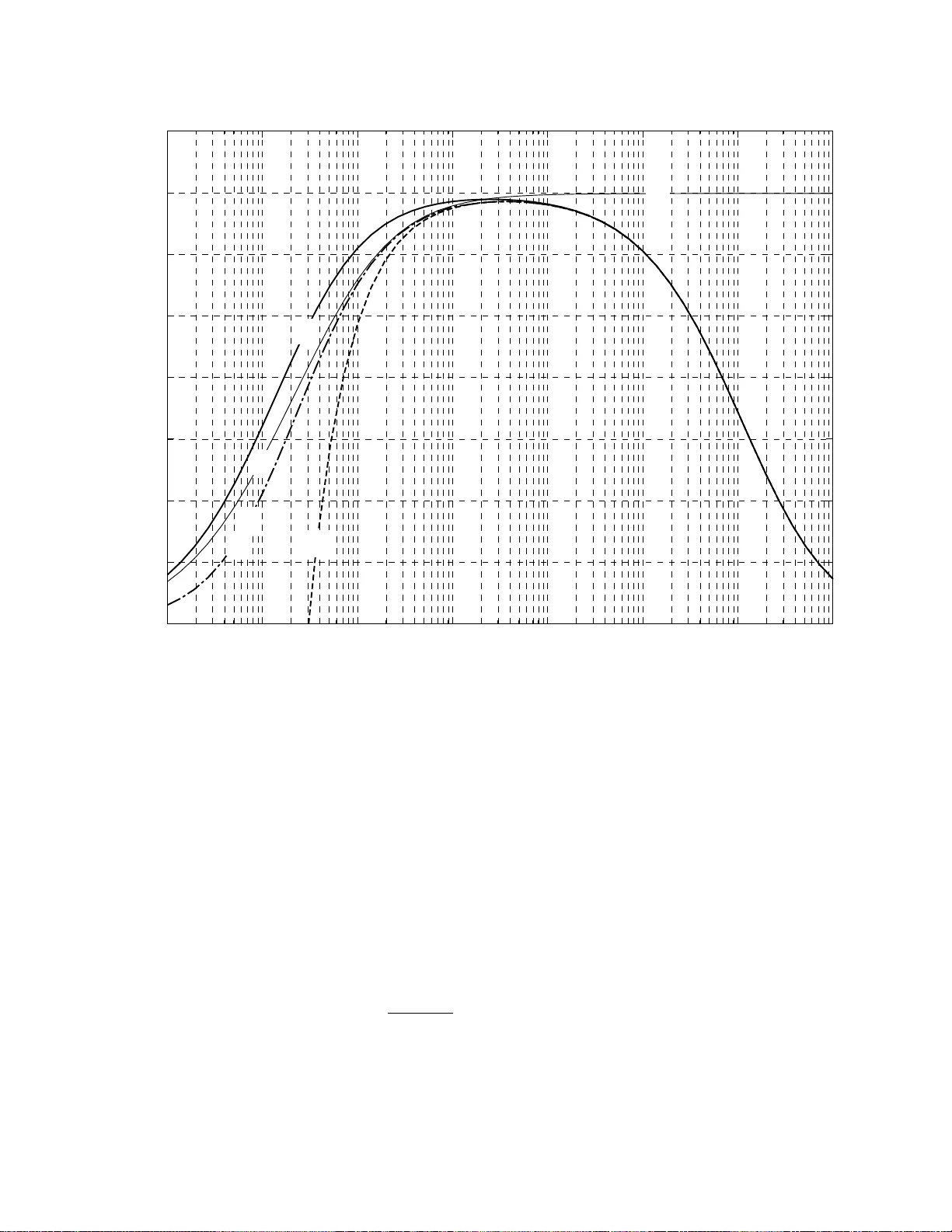
1 Noncoherent Capacity of Underspread F ading Channels Giuseppe Durisi, Member , IEEE, Ulrich G. Schuster , Student Member , IEEE, Helmut B ¨ olcskei, Senior Member , IEEE, Shlomo Shamai (Shitz), F ellow , IEEE Abstract W e deriv e bounds on the noncoherent capacity of wide-sense stationary uncorrelated scattering (WSSUS) channels that are selecti ve both in time and frequency , and are underspread, i.e., the product of the channel’ s delay spread and Doppler spread is small. F or input signals that are peak constrained in time and frequenc y , we obtain upper and lower bounds on capacity that are explicit in the channel’ s scattering function, are accurate for a large range of bandwidth and allow to coarsely identify the capacity-optimal bandwidth as a function of the peak power and the channel’ s scattering function. W e also obtain a closed-form expression for the ﬁrst-order T aylor series expansion of capacity in the limit of large bandwidth, and show that our bounds are tight in the wideband regime. For input signals that are peak constrained in time only (and, hence, allowed to be peaky in frequency), we provide upper and lo wer bounds on the inﬁnite-bandwidth capacity and ﬁnd cases when the bounds coincide and the inﬁnite-bandwidth capacity is characterized exactly . Our lower bound is closely related to a result by V iterbi (1967). The analysis in this paper is based on a discrete-time discrete-frequency approximation of WSSUS time- and frequency-selectiv e channels. This discretization explicitly takes into account the underspread property , which is satisﬁed by virtually all wireless communication channels. This work was supported in part by the Swiss Kommission f ¨ ur T echnologie und Innovation (KTI) under grant 6715.2 ENS-ES, and by the European Commission as part of the Integrated Project P U L S E R S Phase II under contract FP6-027142, and as part of the FP6 Network of Excellence NEWCOM. G. Durisi and H. B ¨ olcskei are with the Communication T echnology Laboratory , ETH Zurich, 8092 Zurich, Switzerland (e-mail: { gdurisi, boelcskei } @nari.ee.ethz.ch). U. G. Schuster was with the Communication T echnology Laboratory , ETH Zurich, and is no w with Celestrius A G, Zurich, Switzerland. S. Shamai (Shitz) is with T echnion, Israel Institute of T echnology , 32000 Haifa, Israel (e-mail: sshlomo@ee.technion.ac.il). This paper was presented in part at the IEEE International Symposium on Information Theory , Seattle, W A, U.S.A., July 2006, and at the IEEE International Symposium on Information Theory , Nice, France, June 2007. November 26, 2024 DRAFT 2 I . I N T R O D U C T I O N A N D O U T L I N E 1) Models for fading channels: Channel capacity is a benchmark for the design of an y communi- cation system. The techniques used to compute, or at least to bound, channel capacity often provide guidelines for the design of practical systems, e.g., ho w to best utilize the resources bandwidth and po wer , and how to design efﬁcient modulation and coding schemes [1, Sec. III.3]. Our goal in this paper is to analyze the capacity of wireless communication channels that are of direct practical importance. W e belie ve that an accurate stochastic model for such channels should take the follo wing aspects into account: • The channel is selecti ve in time and frequency , i.e., it exhibits memory in frequency and in time, respectiv ely . • Neither the transmitter nor the receiver kno ws the instantaneous realization of the channel. • The peak power of the input signal is limited. These aspects are important because they arise from practical limitations of real-world communica- tion systems: temporal variations of the en vironment and multipath propagation are responsible for channel selectivity in time and frequency , respectiv ely [2], [3]; perfect channel knowledge at the recei ver is impossible to obtain because channel state information needs to be extracted from the recei ved signal; ﬁnally , realizable transmitters are al ways limited in their peak output po wer [4]. The abov e aspects are also fundamental as they signiﬁcantly impact the behavior of channel capacity: for example, the capacity of a block-fading channel behav es differently from the capacity of a channel that is stationary in time [5]; channel capacity with perfect channel knowledge at the receiv er is always lar ger than the capacity without channel knowledge [6], and the signaling schemes necessary to achiev e capacity are also very different in the tw o cases [1]; ﬁnally , a peak constraint on the transmit signal can lead to vanishing capacity in the large-bandwidth limit [7]–[9], while without a peak constraint the inﬁnite-bandwidth A WGN capacity can be attained asymptotically [7], [10]–[15]. Small scale fading of wireless channels can be sensibly modeled as a stochastic Gaussian linear time-v arying (L TV) system [2]; in particular , we base our dev elopments on the widely used wide- sense stationary uncorrelated scattering (WSSUS) model for random L TV channels [16], [12]. Like most models for real-world channels, the WSSUS model is time continuous; howe ver , almost all tools for information-theoretic analysis of noisy channels require a discretized representation of the channel’ s input-output relation. Sev eral approaches to discretize random L TV channels are proposed November 26, 2024 DRAFT 3 in the literature, e.g., sampling [8], [16], [17] or basis expansion [18], [19]; all these discretized models incur an approximation error with respect to the continuous-time WSSUS model that is often dif ﬁcult to quantify . As virtually all wireless channels of practical interest are underspr ead , i.e., the product of maximum delay and maximum Doppler shift is small, we b uild our information-theoretic analysis upon a discretization of L TV channels, proposed by K ozek [20], that explicitly takes into account the underspread property to minimize the approximation error in the mean-square sense. 2) Capacity of noncoher ent WSSUS channels: Throughout the paper , we assume that both the transmitter and receiv er know the channel law 1 but both are ignorant of the channel realization, a setting often called noncoher ent . In the following, we refer to channel capacity in the noncoherent setting simply as “capacity”. In contrast, in the coherent setting the recei ver is also assumed to know the channel realization perfectly; the corresponding capacity is termed coherent capacity . A general closed-form expression for the capacity of Rayleigh-fading channels is not known, e ven if the channel is memoryless [22]. Howe v er , sev eral asymptotic results are av ailable. If only a constraint on the average transmitted power is imposed, the A WGN capacity can be achie ved in the inﬁnite-bandwidth limit also in the presence of fading. This result is quite robust, as it holds for a wide variety of channel models [7], [10]–[15]. V erd ´ u showed that ﬂash signaling , which implies unbounded peak power of the input signal, is necessary and sufﬁcient to achiev e the inﬁnite- bandwidth A WGN capacity on block-memoryless fading channels [14]; a form of ﬂash signaling is also inﬁnite-bandwidth optimal for the more general time- and frequency-selecti ve channel model used in the present paper [15]. In contrast, if the peakiness of the input signal is restricted, the inﬁnite-bandwidth capacity behavior of most fading channels changes drastically , and the limit depends on the type of peak constraint imposed [7]–[9], [13], [23]. In this paper , we shall distinguish between a peak constraint in time and a peak constraint in time and frequency . a) P eak constraint in time: No closed-form capacity expression, not ev en in the inﬁnite- bandwidth limit, seems to e xist to date for time- and frequency-selectiv e WSSUS channels. V iterbi’ s analysis [23] provides a result that can be interpr eted as a lower bound on the inﬁnite-bandwidth capacity of time- and frequency-selecti ve channels. This lower bound is in the form of the inﬁnite- bandwidth A WGN capacity minus a penalty term that depends on the channel’ s power -Doppler 1 This implies that the codebook and the decoding strategy can be optimized accordingly [21]. November 26, 2024 DRAFT 4 proﬁle [16]. For channels that are time selecti ve but frequency ﬂat, structurally similar expressions were found for the inﬁnite-bandwidth capacity [24], [25] and for the capacity per unit energy [26]. b) P eak constraint in time and fr equency: Although a closed-form capacity expression valid for all bandwidths is not av ailable, it is known that the inﬁnite-bandwidth capacity is zero for v arious channel models [7]–[9]. This asymptotic capacity behavior implies that signaling schemes that spread the transmit energy uniformly across time and frequency perform poorly in the large- bandwidth regime. Even more useful for performance assessment would be capacity bounds for ﬁnite bandwidth. For frequenc y-ﬂat time-selecti ve channels, such bounds can be found in [27], [28], while for the more general time- and frequency-selecti v e case treated in the present paper , upper bounds seem to exist only on the rates achiev able with particular signaling schemes, namely for orthogonal frequency-di vision multiplexing (OFDM) with constant-modulus symbols [29], and for multiple-input multiple-output (MIMO) OFDM with unitary space-frequency codes over frequency-selecti ve block-fading channels [30]. 3) Contributions: W e use the discrete-time discrete-frequenc y approximation of continuous-time underspread WSSUS channels proposed in [20], to obtain the following results: • W e deriv e upper and lower bounds on capacity under a constraint on the average po wer and under a peak constraint in both time and frequency . These bounds are valid for any bandwidth, are explicit in the channel’ s scattering function, and generalize the results on achiev able rates in [29]. In particular , our bounds allow to coarsely identify the capacity-optimal bandwidth for a giv en peak constraint and a giv en scattering function. • Under the same peak constraint in time and frequency , we ﬁnd the ﬁrst-order T aylor series expansion of channel capacity in the limit of inﬁnite bandwidth. This result e xtends the asymptotic capacity analysis for frequency-ﬂat time-selecti v e channels in [28] to channels that are selectiv e in both time and frequency . • In the inﬁnite-bandwidth limit and for transmit signals that are peak-constrained in time only , we recover V iterbi’ s capacity lower bound [23]. In addition, we derive an upper bound that is sho wn to coincide with the lower bound for a speciﬁc class of channels; hence, the inﬁnite- bandwidth capacity for this class of channels is established. The results in this paper rely on se veral ﬂav ors of Szeg ¨ o’ s theorem on the asymptotic eigen value distribution of T oeplitz matrices [31], [32]; in particular , we use v arious extensions of Sze g ¨ o’ s theorem to two-level T oeplitz matrices, i.e., block-T oeplitz matrices that hav e T oeplitz blocks [33], November 26, 2024 DRAFT 5 [34]. Another key ingredient for several of our proofs is the relation between mutual information and minimum mean-square error (MMSE) discovered recently by Guo et al. [35]. Furthermore, we use a property of the information div ergence of orthogonal signaling schemes deriv ed by Butman and Klass [36]. 4) Notation: Uppercase boldface letters denote matrices and lowercase boldface letters designate vectors. The superscripts T , ∗ , and H stand for transposition, element-wise conjugation, and Hermitian transposition, respectiv ely . For two matrices A and B of appropriate dimensions, the Hadamard pr oduct is denoted as A  B . W e designate the identity matrix of dimension N × N as I N and the all-zero vector of appropriate dimension as 0 . W e let diag ( x ) denote a diagonal square matrix whose main diagonal contains the elements of the vector x . The determinant, trace, and rank of the matrix X are denoted as det( X ) , tr( X ) , and rank( X ) , respecti vely , and λ i ( X ) is the i th eigen value of a square matrix X . The function δ ( x ) is the Dirac distribution, and δ [ n ] is deﬁned as δ [0] = 1 and δ [ n ] = 0 for all n 6 = 0 . All logarithms are to the base e . The real part of the complex number z is denoted <{ z } . W e write A −B for the set difference between the sets A and B . For two functions f ( x ) and g ( x ) , the notation f ( x ) = o ( g ( x )) for x → 0 means that lim x → 0 f ( x ) /g ( x ) = 0 . W ith b x c we denote the largest integer smaller or equal to x ∈ R . A signal is an element of the Hilbert space L 2 of square integrable functions. The inner product between two signals f ( x ) and g ( x ) is denoted as h f , g i = R ∞ −∞ f ( x ) g ∗ ( x ) dx . For a random variable (R V) x with distribution Q x , we write x ∼ Q x . W e denote expectation by E [ · ] , and use the notation E x [ · ] to stress that the expectation is taken with respect to the R V x . W e write D ( Q x k Q y ) for the Kullback-Leibler (KL) div er gence between the two distributions Q x and Q y . Finally , C N ( m , R ) stands for the distribution of a jointly proper Gaussian (JPG) random vector with mean m and cov ariance matrix R . I I . C H A N N E L A N D S Y S T E M M O D E L A channel model needs to strike a balance between generality , accuracy , engineering relev ance, and mathematical tractability . In the following, we start from the classical WSSUS model for L TV channels [16], [12] because it is a fairly general, yet accurate and mathematically tractable model that is widely used. This model has a continuous-time input-output relation, which is dif ﬁcult to use as a basis for information-theoretic studies. Ho we ver , if the channel is underspr ead it is possible to closely approximate the original WSSUS input-output relation by a discretized input- output relation that is especially suited for the deri vation of capacity bounds. In particular , the bounds November 26, 2024 DRAFT 6 we deriv e in this paper can be directly related to the underlying continuous-time WSSUS channel as they are explicit in its scattering function. A. T ime- and F r equency-Selective Underspr ead F ading Channels 1) The channel operator: A wireless channel can be described as a linear operator H : L 2 → R H that maps an input signal x ( t ) into an output signal r ( t ) ∈ R H , where R H ⊂ L 2 denotes the range space of H [37]. The corresponding noise-free input-output relation is then r ( t ) = ( H x )( t ) . It is sensible to model wireless channels as random, for one because a deterministic description of the physical propagation en vironment is too complex in most cases of practical interest, and second because a stochastic description is much more robust, in the sense that systems designed on the basis of a stochastic channel model can be expected to work in a variety of dif ferent propagation en vironments [3]. Consequently , we assume that H is a random operator . 2) System functions: Because communication takes place over a ﬁnite bandwidth and a ﬁnite time duration, we can assume that each realization of H is a Hilbert-Schmidt operator [38], [39]. Hence, the noise-free input-output relation of the L TV channel can be written as 2 [38, p. 1083] r ( t ) =  H x  ( t ) = Z t 0 k H ( t, t 0 ) x ( t 0 ) dt 0 (1) where the kernel k H ( t, t 0 ) can be interpreted as the channel response at time t to a Dirac impulse at time t 0 . Instead of two variables that denote absolute time, it is common in the engineering literature to use absolute time t and delay τ . This leads to the time-varying impulse response h H ( t, τ ) = k H ( t, t − τ ) and the corresponding noise-free input-output relation [16] r ( t ) = Z τ h H ( t, τ ) x ( t − τ ) dτ . (2) T wo more system functions that will be important in the follo wing dev elopments are the time-varying transfer function 3 L H ( t, f ) = Z τ h H ( t, τ ) e − j 2 π f τ dτ (3) 2 All integrals are from −∞ to ∞ unless stated otherwise. 3 As H is of Hilbert-Schmidt type, the time-varying impulse response h H ( t, τ ) is square integrable, and the Fourier transforms in (3) and (4) are well deﬁned. November 26, 2024 DRAFT 7 and the spr eading function S H ( ν, τ ) = Z t h H ( t, τ ) e − j 2 π ν t dt = Z Z t f L H ( t, f ) e − j 2 π ( ν t − τ f ) dtd f . (4) In particular , if we rewrite the input-output relation (2) in terms of the spreading function S H ( ν, τ ) as r ( t ) = Z Z ν τ S H ( ν, τ ) x ( t − τ ) e j 2 π tν dτ dν (5) we obtain an intuitiv e physical interpretation: the output signal r ( t ) is a weighted superposition of copies of the input signal x ( t ) that are shifted in time by the delay τ and in frequency by the Doppler shift ν . 3) Stoc hastic characterization and WSSUS assumption: For mathematical tractability , we need to make additional assumptions on the system functions. First, we assume that L H ( t, f ) is a zero- mean JPG random process in t and f . Indeed, the Gaussian distribution is empirically supported for narrowband channels [2], and e ven ultrawideband (UWB) channels with bandwidth up to se veral gigahertz can be modeled as Gaussian distributed [40]. By virtue of the Gaussian assump- tion, L H ( t, f ) is completely characterized by its correlation function. Y et, this correlation function is four-dimensional in general and thus difﬁcult to work with. A further simpliﬁcation is possible if we assume that the channel process is wide-sense stationary in time t and uncorr elated in delay τ , the so-called WSSUS assumption [16]. As a consequence, L H ( t, f ) is wide-sense stationary both in time t and frequency f , or , equiv alently , S H ( ν, τ ) is uncorrelated in Doppler ν and delay τ [16]: E [ L H ( t, f ) L ∗ H ( t 0 , f 0 )] = R H ( t − t 0 , f − f 0 ) E [ S H ( ν, τ ) S ∗ H ( ν 0 , τ 0 )] = C H ( ν, τ ) δ ( ν − ν 0 ) δ ( τ − τ 0 ) . The function R H ( t, f ) is called the channel’ s (time-frequency) correlation function, and C H ( ν, τ ) is called the scattering function of the channel H . The two functions are related by a two-dimensional Fourier transform, C H ( ν, τ ) = Z Z t f R H ( t, f ) e − j 2 π ( ν t − τ f ) dtd f . (6) November 26, 2024 DRAFT 8 As R H ( t, f ) is stationary in t and f , C H ( ν, τ ) is nonnegati ve and real-valued for all ν and τ , and can be interpreted as the spectrum of the channel process. The power-delay pr oﬁle of H is deﬁned as p H ( τ ) = Z ν C H ( ν, τ ) dν and the power-Doppler pr oﬁle as q H ( ν ) = Z τ C H ( ν, τ ) dτ . The WSSUS assumption is widely used in wireless channel modeling [16], [12], [2], [1], [41], [42]. It is in good agreement with measurements of tropospheric scattering channels [12], and provides a reasonable model for many types of mobile radio channels [43]–[45], at least over a limited time duration and bandwidth [16]. Furthermore, the scattering function can be directly estimated from measured data [46], [47], so that capacity expressions and bounds that e xplicitly depend on the channel’ s scattering function can be ev aluated for many channels of practical interest. Formally , the WSSUS assumption is mathematically incompatible with the requirement that H is of Hilbert-Schmidt type, or , equiv alently , that the system functions are square integrable, because sta- tionarity in time t and frequenc y f of L H ( t, f ) implies that L H ( t, f ) cannot decay to zero for t → ∞ and f → ∞ . Similarly to the engineering model of white noise, this incompatibility is a mathematical artifact and not a problem of real-world wireless channels: in fact, ev ery communication system transmits ov er a ﬁnite time duration and ov er a ﬁnite bandwidth. 4 W e believ e that the simpliﬁcation the WSSUS assumption entails justiﬁes this mathematical inconsistency . B. The Underspr ead Assumption and its Consequences Because the velocity of the transmitter , of the recei ver , and of the objects in the propagation en vironment is limited, so is the maximum Doppler shift ν 0 experienced by the transmitted signal. W e also assume that the maximum delay is strictly smaller than 2 τ 0 . For simplicity and without loss of generality , throughout this paper , we consider scattering functions that are centered at τ = 0 and ν = 0 , i.e., we remove an y ov erall ﬁxed delay and Doppler shift. The assumptions of limited 4 A more detailed account on solutions to overcome the mathematical incompatibility between stationary and ﬁnite-energy models can be found in [48, Sec. 7.5]. November 26, 2024 DRAFT 9 Doppler shift and delay then imply that the scattering function is supported on a rectangle of spr ead ∆ H = 4 ν 0 τ 0 , C H ( ν, τ ) = 0 for ( ν , τ ) / ∈ [ − ν 0 , ν 0 ] × [ − τ 0 , τ 0 ] . (7) Condition (7) in turn implies that the spreading function S H ( ν, τ ) is also supported on the same rectangle with probability 1 ( w .p.1 ). If ∆ H < 1 , the channel is said to be underspr ead [16], [12], [20]. V irtually all channels in wireless communication are highly underspread, with ∆ H ≈ 10 − 3 for typical land-mobile channels and as lo w as 10 − 7 for some indoor channels with restricted mobility of the terminals [49]–[51]. The underspread property of typical wireless channels is very important, ﬁrst because only (deterministic) underspread channels can be completely identiﬁed from measurements [52], [53], and second because underspread channels hav e a well-structured set of approximate eigenfunctions that can be used to discretize the channel operator , as described next. 1) Appr oximate diagonalization of underspr ead channels: As H is a Hilbert-Schmidt operator , its kernel can be expressed in terms of its positi ve singular values { σ i } , its left singular functions { u i ( t ) } , and its right singular functions { v i ( t ) } [37, Th. 6.14.1], according to k H ( t, t 0 ) = ∞ X i = −∞ σ i u i ( t ) v ∗ i ( t 0 ) . (8) W e denote by N H the null space of H , i.e., the space of input signals that the channel maps onto 0 . The set { v i ( t ) } is an orthonormal basis for the linear span of L 2 − N H , and { u i ( t ) } is an orthonormal basis for the range space R H . Any input signal in N H is of no utility for communication purposes; the remaining input signals in the linear span of L 2 − N H , which we denote in the remainder of the paper as input space , can be completely characterized by their projections onto the set { v i ( t ) } . Similarly , the output signal r ( t ) = ( H x )( t ) is completely described by its projections onto the set { u i ( t ) } . These projections together with the kernel decomposition (8) yield a countable set of scalar input-output relations, which we refer to as the diagonalization of H . Because the right and left singular functions depend on the realization of H , diagonalization requires perfect channel knowledge. But this knowledge is not av ailable in the noncoherent setting. In contrast, if the singular functions of the random channel H did not depend on its particular realization, we could diagonalize H without knowledge of the channel realization. This is the case, for example, for random linear time-in variant (L TI) channels, where complex sinusoids are always eigenfunctions, independently of the realization of the channel’ s impulse response. Fortunately , the November 26, 2024 DRAFT 10 singular functions of underspread random L TV channels can be well approximated by deterministic functions. More precisely , an underspread channel H has the following properties [20]: 1) All realizations of the underspread channel H are approximately normal , so that the singular v alue decomposition (8) can be replaced by an eigen value decomposition. 2) Any deterministic unit-energy signal g ( t ) that is well localized 5 in time and frequency is an appr oximate eigenfunction of H in the mean-square sense, i.e., the mean-square error E [ kh H g , g i g − H g k 2 ] is small if H is underspread. This error can be further reduced by an appropriate choice of g ( t ) , where the choice depends on the scattering function C H ( ν, τ ) . 3) If g ( t ) is an approximate eigenfunction as deﬁned in the previous point, then so is g ( α,β ) ( t ) = g ( t − α ) e j 2 π β t for any time shift α ∈ R and any frequency shift β ∈ R . 4) For an y ( α, β ) , the time-v arying transfer function L H ( α, β ) is an appr oximate eigen value of H corresponding to the approximate eigenfunction g ( α,β ) ( t ) , in the sense that the mean-square error E    h H g ( α,β ) , g ( α,β ) i − L H ( α, β )   2  is small. W e use these properties of underspread operators to construct an approximation e H of the random channel H that has a well-structured set of deterministic eigenfunctions. The errors incurred by this approximation are discussed in detail in Appendix A. W e then diagonalize this approximating operator and exclusi vely consider the corresponding discretized input-output relation in the reminder of the paper . Property 1, the approximate normality of H , together with Property 2 implies that the kernel of the approximating operator e H can be synthesized as P ∞ i = −∞ λ i z i ( t ) z ∗ i ( t 0 ) , where, dif ferently from (8), the λ i are now random eigen values instead of random singular values, and the z i ( t ) constitute a set of deterministic orthonormal eigenfunctions instead of random singular functions. Property 2 means that we are at liberty to choose the approximate eigenfunctions z i ( t ) among all signals that are well localized in time and frequency . In particular , we would like the result- ing approximating kernel to be conv enient to work with and the approximate eigenfunctions z i ( t ) easy to implement, as discussed in Section II-B 3; therefore, we choose the set of approximate eigenfunctions to be highly structured. By Property 3, it is possible to use time- and frequency- shifted versions of a single well-localized prototype function g ( t ) as eigenfunctions. Furthermore, because the support of S H ( ν, τ ) is strictly limited in Doppler ν and delay τ , it follows from the 5 W e measure the joint time-frequency localization of a signal g ( t ) by the product between its effective duration and its effective bandwidth , deﬁned in (64). November 26, 2024 DRAFT 11 sampling theorem and the Fourier transform relation (4) that the samples L H ( k T , nF ) , taken on a rectangular grid with T ≤ 1 / (2 ν 0 ) and F ≤ 1 / (2 τ 0 ) , are sufﬁcient to characterize L H ( t, f ) exactly . Hence, we take as our set of approximate eigenfunctions the so-called W e yl-Heisenber g set { g k,n ( t ) } , where g k,n ( t ) = g ( t − k T ) e j 2 π nF t are orthonormal signals. The requirement that the g k,n ( t ) are orthonormal and at the same time well localized in time and frequency implies T F > 1 [54], as a consequence of the Balian-Low theorem [55, Ch. 8]. Large values of the product T F allo w for better time-frequency localization of g ( t ) , but result in a loss of dimensions in signal space compared with the critically sampled case T F = 1 . The Nyquist condition T ≤ 1 / (2 ν 0 ) and F ≤ 1 / (2 τ 0 ) can be readily satisﬁed for all underspread channels. The samples L H ( k T , nF ) are approximate eigen v alues of H by Property 4; hence, our choice of approximate eigenfunctions results in the following approximating eigen v alue decomposition for k H ( t, t 0 ) k H ( t, t 0 ) ≈ k e H ( t, t 0 ) = ∞ X k = −∞ ∞ X n = −∞ L H ( k T , nF ) g k,n ( t ) g ∗ k,n ( t 0 ) (9) where k e H ( t, t 0 ) denotes the kernel of the approximating operator e H . For T F > 1 , the W eyl- Heisenberg set { g k,n ( t ) } is not complete in L 2 [54, Th. 8.3.1]. Therefore, the null space of e H is nonempty . As k e H ( t, t 0 ) is only an approximation of k H ( t, t 0 ) , this null space might dif fer from N H . Similarly , the range space of e H might dif fer from R H . The characterization of the difference between these spaces is an important open problem. 2) Canonical characterization of signaling schemes: The approximating random channel opera- tor e H has a highly structured set of deterministic orthonormal eigenfunctions. W e can, therefore, diagonalize the input-output relation of the approximating channel without the need for channel kno wledge at both transmitter and recei ver . Any input signal x ( t ) that lies in the input space of the approximating operator is uniquely characterized by its projections onto the set { g k,n ( t ) } . All physically realizable transmit signals are effectively band limited . As the prototype function g ( t ) is well concentrated in frequency by construction, we can model the effecti ve band limitation of x ( t ) by using only a ﬁnite number of slots N in frequency . The resulting transmitted signal x ( t ) = ∞ X k = −∞ N − 1 X n =0 h x, g k,n i | {z } = x [ k,n ] g k,n ( t ) (10) then has effecti ve bandwidth W = N F . W e call the coefﬁcient x [ k , n ] the transmit symbol in the time-fr equency slot ( k , n ) . The received signal can be expanded in the same basis. T o compute the November 26, 2024 DRAFT 12 resulting projections, we substitute k e H ( t, t 0 ) and the canonical input signal (10) into the integral input-output relation (1), add white Gaussian noise w ( t ) , and project the resulting noisy receiv ed signal y ( t ) = ( e H x )( t ) + w ( t ) onto the functions { g k,n ( t ) } , i.e., y [ k , n ] = h y , g k,n i = h e H x, g k,n i + h w , g k,n i | {z } w [ k ,n ] = X k 0 ,n 0 x [ k 0 , n 0 ] h e H g k 0 ,n 0 , g k,n i + w [ k , n ] = L H ( k T , nF ) | {z } h [ k,n ] x [ k , n ] + w [ k , n ] (11) for all time-frequency slots ( k , n ) . The last step in (11) follo ws from the orthonormality of the set { g k,n ( t ) } . Orthonormality also implies that the discretized noise signal w [ k , n ] is JPG, indepen- dent and identically distributed (i.i.d.) ov er time k and frequency n ; for con venience, we normalize the noise variance so that w [ k , n ] ∼ C N (0 , 1) for all k and n . The diagonalized input-output relation (11) is completely generic, i.e., it is not limited to a speciﬁc signaling scheme. 3) OFDM interpr etation of the appr oximating channel model: The canonical signaling scheme (10) and the corresponding discretized input-output relation (11), are not just tools to analyze channel capacity , but also lead to a practical transmission system. The decomposition of the channel input signal (10) can be interpreted as pulse-shaped (PS) OFDM [56], where discrete data symbols x [ k , n ] are modulated onto a set of orthogonal signals, indexed by k and n . In addition, this perspectiv e leads to an operational interpretation of the error incurred when approximating k H ( t, t 0 ) as in (9). The time- and frequency-dispersi ve nature of L TV channels leads to intersymbol interference (ISI) and intercarrier interference (ICI) in the receiv ed PS-OFDM signal. This is apparent if we project r ( t ) onto the function g k,n ( t ) : h r , g k,n i = h H x, g k,n i = ∞ X k 0 = −∞ N − 1 X n 0 =0 x [ k 0 , n 0 ] h H g k 0 ,n 0 , g k,n i = h H g k,n , g k,n i x [ k , n ] + ∞ X k 0 = −∞ N − 1 X n 0 =0 ( k 0 ,n 0 ) 6 =( k,n ) x [ k 0 , n 0 ] h H g k 0 ,n 0 , g k,n i . (12) The second term on the right-hand side (RHS) of (12) corresponds to ISI and ICI, while the ﬁrst term is the desired signal; we can approximate the ﬁrst term as L H ( k T , nF ) x [ k , n ] by Property 4. Comparison of (11) and (12) then sho ws that the input-output relation (11), which results from the November 26, 2024 DRAFT 13 approximation (9), can be interpreted as PS-OFDM transmission over the original channel H if all ISI and ICI terms are neglected. W ith proper design of the prototype signal g ( t ) and choice of the grid parameters T and F , both ISI and ICI can be reduced [56]–[58]. The larger the product T F , the more ef fectiv e the reduction in ISI and ICI, as discussed in Appendix A. Heuristically , a good compromise between loss of dimensions in signal space and reduction of the interference terms seems to result for T F ' 1 . 2 [56], [58]. The cyclic preﬁx (CP) in a con ventional CP-OFDM system incurs a similar dimension loss. In (72) , we provide an upper bound on mean-square energy of the interference term in (12), and sho w ho w this upper bound can be minimized by a careful choice of the signal g ( t ) and of the grid parameters T and F [20], [17], [58]. For general scattering functions, the optimization of the triple { g ( t ) , T , F } needs to be performed numerically; a general guideline is to choose T and F such that (see Appendix A) T F = τ 0 ν 0 . (13) T o summarize, in this section we constructed an approximation e H of the random linear operator H on the basis of the underspread property . The kernel of the approximating operator is synthesized from the W eyl-Heisenber g set { g k,n ( t ) } as in (9) , so that { g k,n ( t ) } is an orthonormal basis for the input space and the range space of e H . The decomposition of the input signal (10) can be interpreted as PS-OFDM: this interpretation sheds light on one of the errors resulting from the approximation (9) . Finally , an important open problem is the characterization of the dif ference between the input spaces of H and e H , and between the range spaces of H and e H . C. Linear T ime-In variant and Linear F requency-In variant Channels The properties of L TV underspread channels we listed in Section II-B are similar to the properties of L TI and linear frequency-in variant (LFI) channels: both L TI and LFI channel operators are normal and ha ve a well-structured set of deterministic eigenfunctions (sinusoids parametrized by frequency for L TI channels, and Dirac functions parametrized by time for LFI channels), with corresponding eigen values equal to the samples of a channel system function (e.g., the transfer function in the L TI case). Intuitiv ely , L TI and LFI channels are limiting cases within the class of L TV channels analyzed in this section; in fact, an L TV channel reduces to an L TI channel when ν 0 = 0 , and to an LFI channel when τ 0 = 0 . Both L TI and LFI channels are then underspread, according to our November 26, 2024 DRAFT 14 deﬁnition. Y et, since L TI and LFI channel operators are not of Hilbert-Schmidt type [59, App. A], the kernel diagonalization presented in Section II-B does not apply to these two classes of channels; consequently , the capacity bounds we deri v e in Sections III and IV do not reduce to capacity bounds for the L TI or the LFI case when ν 0 = 0 or τ 0 = 0 , respectively . 6 Quasi-L TI channels, i.e., channels that are slowly time varying ( ν 0 small but positi ve), and quasi- LFI channels, i.e., channels that are slowly frequency v arying ( τ 0 small but positi ve), can instead be approximately diagonalized as described in Section II-B, as long as they are underspread. D. Discr ete-T ime Discrete-F r equency Input-Output Relation The discrete-time discrete-frequency channel coefﬁcients { h [ k , n ] } constitute a two-dimensional discrete-parameter stationary random process that is JPG with zero mean and correlation function R H [ k , n ] = E [ h [ k 0 + k , n 0 + n ] h ∗ [ k 0 , n 0 ]] = E  L H  ( k 0 + k ) T , ( n 0 + n ) F  L ∗ H ( k 0 T , n 0 F )  . (14) The two-dimensional power spectral density of { h [ k , n ] } is deﬁned as c ( θ , ϕ ) = ∞ X k = −∞ ∞ X n = −∞ R H [ k , n ] e − j 2 π ( kθ − nϕ ) , | θ | , | ϕ | ≤ 1 / 2 . (15) W e shall often need the follo wing e xpression for c ( θ , ϕ ) in terms of the scattering function C H ( ν, τ ) : c ( θ , ϕ ) ( a ) = ∞ X k = −∞ ∞ X n = −∞ e − j 2 π ( kθ − nϕ ) Z Z ν τ C H ( ν, τ ) e j 2 π ( kT ν − nF τ ) dτ dν = Z Z ν τ C H ( ν, τ ) ∞ X k = −∞ e j 2 π kT ( ν − θ T ) ∞ X n = −∞ e − j 2 π nF ( τ − ϕ F ) dτ dν ( b ) = 1 T F Z Z ν τ C H ( ν, τ ) ∞ X k = −∞ δ  ν − θ − k T  ∞ X n = −∞ δ  τ − ϕ − n F  dτ dν = 1 T F ∞ X k = −∞ ∞ X n = −∞ C H  θ − k T , ϕ − n F  (16) 6 For deterministic L TI channels, a channel discretization that is useful for information-theoretic analysis is discussed in [13, Sec. 8.5]. November 26, 2024 DRAFT 15 where (a) follo ws from the F ourier transform relation (6), and (b) results from Poisson’ s summation formula. The variance of each channel coefﬁcient is giv en by σ 2 H = 1 / 2 Z − 1 / 2 1 / 2 Z − 1 / 2 c ( θ , ϕ ) dθ dϕ ( a ) = 1 T F ∞ X k = −∞ ∞ X n = −∞ 1 / 2 Z − 1 / 2 1 / 2 Z − 1 / 2 C H  θ − k T , ϕ − n F  dθ dϕ ( b ) = 1 T F 1 / 2 Z − 1 / 2 1 / 2 Z − 1 / 2 C H  θ T , ϕ F  dθ dϕ ( c ) = Z Z ν τ C H ( ν, τ ) dτ dν (17) where (a) follows from (16), and (b) results because we chose the grid parameters to satisfy the Nyquist conditions T ≤ 1 / (2 ν 0 ) and F ≤ 1 / (2 τ 0 ) , so that periodic repetitions of the compactly supported scattering function lie outside the integration region. Finally , (c) follows from the change of v ariables ν = θ /T and τ = ϕ/F . For ease of notation, we normalize σ 2 H = 1 throughout the paper . For each time slot k , we arrange the discretized input signal x [ k , n ] , the discretized output signal y [ k , n ] , the channel coefﬁcients h [ k , n ] , and the noise samples w [ k , n ] in corresponding vectors. F or example, the N -dimensional vector that contains the input symbols in the k th time slot is deﬁned as x [ k ] = h x [ k , 0] x [ k , 1] · · · x [ k , N − 1] i T . The output vector y [ k ] , the channel vector h [ k ] , and the noise vector w [ k ] are deﬁned analogously . This notation allows us to rewrite the input-output relation (11) as y [ k ] = h [ k ]  x [ k ] + w [ k ] (18) November 26, 2024 DRAFT 16 for all k . In this formulation, the channel is a multiv ariate stationary process { h [ k ] } with matrix- v alued correlation function R h [ k ] = E  h [ k 0 + k ] h H [ k 0 ]  =        R H [ k , 0] R ∗ H [ k , 1] . . . R ∗ H [ k , N − 1] R H [ k , 1] R H [ k , 0] . . . R ∗ H [ k , N − 2] . . . . . . . . . . . . R H [ k , N − 1] R H [ k , N − 2] . . . R H [ k , 0]        . (19) In most of the following analyses, we initially consider a ﬁnite number K of time slots and then take the limit K → ∞ . T o obtain a compact notation, we stack K contiguous elements of the multi variate input, channel, and output processes just deﬁned. For the channel input, this results in the K N -dimensional vector x = h x T [0] x T [1] · · · x T [ K − 1] i T . (20) Again, the stacked vectors y , h , and w are deﬁned analogously . W ith these deﬁnitions, we can now compactly express the input-output relation (11) as y = x  h + w . (21) W e denote the correlation matrix of the stacked channel vector h by R h = E  hh H  . Because the channel process { h [ k , n ] } is stationary in time and in frequency , R h is a two-le vel Hermitian T oeplitz matrix, giv en by R h =        R h [0] R H h [1] . . . R H h [ K − 1] R h [1] R h [0] . . . R H h [ K − 2] . . . . . . . . . . . . R h [ K − 1] R h [ K − 2] . . . R h [0]        . (22) E. P ower Constraints Throughout the paper , we assume that the average po wer of the transmitted signal is constrained as (1 /T ) E [ k x k 2 ] ≤ K P . In addition, we limit the peak po wer to be no lar ger than β times the av erage power , where β ≥ 1 is the nominal peak- to average-power ratio (P APR). The multi v ariate input-output relation (21) allows to constrain the peak po wer in se veral different ways. W e analyze the following two cases: November 26, 2024 DRAFT 17 1) P eak constraint in time: The power of the transmitted signal in each time slot k is limited as 1 T N − 1 X n =0 | x [ k , n ] | 2 ≤ β P w .p.1 . (23) This constraint models the fact that physically realizable power ampliﬁers can only provide limited output power [4]. 2) P eak constraint in time and fr equency: Regulatory bodies sometimes limit the peak power in certain frequenc y bands, e.g., for UWB systems. W e model this type of constraint by imposing a limit on the squared amplitude of the transmitted symbols x [ k , n ] in each time-frequency slot ( k , n ) according to (1 /T ) | x [ k , n ] | 2 ≤ β P / N w .p.1 . (24) This type of constraint is more stringent than the peak constraint in time given in (23). Both peak constraints abov e are imposed on the input symbols x [ k , n ] , i.e., in the eigenspace of the approximating channel operator . This limitation is mathematically con venient; howe ver , the peak v alue of the corresponding transmitted continuous-time signal x ( t ) in (10) also depends on the prototype signal g ( t ) , so that a limit on x [ k , n ] does not generally imply that x ( t ) is peak limited. I I I . C A P A C I T Y B O U N D S U N D E R A P E A K C O N S T R A I N T I N T I M E A N D F R E Q U E N C Y In the present section, we analyze the capacity of the discretized channel in (11) subject to the peak constraint in time and frequency speciﬁed by (24). The link between the discretized channel (11) and the continuous-time channel model established in Section II then allows us to express the resulting bounds in terms of the scattering function C H ( ν, τ ) of the underspread WSSUS channel H . As we assumed that the channel process { h [ k , n ] } has a spectral densit y [giv en in (16) ], the vector process { h [ k ] } is ergodic [60] and the capacity of the discretized underspread channel (21) is gi ven by [61, Ch. 12] C ( W ) = lim K →∞ 1 K T sup Q I ( y ; x ) [nat/s] (25) for a giv en bandwidth W = N F . Here, the supremum is taken over the set Q of all input distributions that satisfy the peak constraint (24) and the av erage-power constraint E [ k x k 2 ] ≤ K P T . The capacity of fading channels with ﬁnite bandwidth has so far resisted all attempts at closed-form solutions [62], [22], [63], ev en for the memoryless case; thus, we resort to bounds to characterize the capacity (25). In particular , we present the following bounds: November 26, 2024 DRAFT 18 • An upper bound U c ( W ) , which we refer to as coherent upper bound, that is based on the assumption that the receiver has perfect knowledge of the channel realizations. This bound is standard; it turns out to be useful for small bandwidth. • An upper bound U 1 ( W ) that is useful for medium to lar ge bandwidth. This bound is explicit in the channel’ s scattering function and extends the upper bound [28, Prop. 2.2] on the capacity of frequency-ﬂat time-selectiv e channels to general underspread channels that are selectiv e in time and frequency . • A lower bound L 1 ( W ) that extends the lower bound [27, Prop. 2.2] to general underspread channels that are selecti v e in time and frequenc y . This bound is explicit in the channel’ s scattering function only for large bandwidth. A. Coher ent Upper Bound The assumption that the receiv er perfectly knows the instantaneous channel realizations furnishes the following capacity upper bound: 1 K T sup Q I ( y ; x ) ( a ) ≤ 1 K T sup Q I ( y ; x | h ) ( b ) ≤ 1 K T sup E [ k x k 2 ] ≤ K P T I ( y ; x | h ) ( c ) = 1 K T sup R x E h  log det  I K N + ( hh H )  R x  ( d ) ≤ N T E h  log  1 + P T N | h | 2  . (26) Here, (a) holds because the coherent mutual information, I ( y ; x | h ) , is an upper bound on the corresponding mutual information in the noncoherent setting. Inequality (b) follows as we drop the peak constraint and thus enlarge the set of admissible input distributions. The supremum of I ( y ; x | h ) ov er the resulting relaxed input constraint is achiev ed by a zero-mean JPG input vector x with cov ariance matrix R x = E  xx H  that satisﬁes tr( R x ) ≤ K P T [3]. T o obtain (c), we use that, conditioned on h , the output vector y is JPG and its cov ariance matrix can be expressed as E  yy H | h  = I K N + E x  ( x  h )( x  h ) H  = I K N + ( hh H )  R x where the last equality results from the following elementary relation between Hadamard products and outer products: ( x  h )( x  h ) H = xx H  hh H . (27) November 26, 2024 DRAFT 19 Finally , (d) follows from Hadamard’ s inequality , from the fact that by Jensen’ s inequality the supremum is achiev ed by R x = ( P T / N ) I K N , and because the channel coefﬁcients all hav e the same distribution h [ k , n ] ∼ h ∼ C N (0 , 1) . As the upper bound (26) does not depend on K , we obtain an upper bound U c ( W ) on capacity (25) as a function of bandwidth W if we set W = N F : C ( W ) ≤ U c ( W ) = W T F E h  log  1 + P T F W | h | 2  . (28) For a discretization of the WSSUS channel H dif ferent from the one in Section II-B , M ´ edard and Gallager [8] showed that the corresponding capacity v anishes with increasing bandwidth if the peakiness of the input signal is constrained in a w ay that includes our peak constraint (24). As the upper bound U c ( W ) monotonically increases in W , it is sensible to conclude that U c ( W ) does not accurately reﬂect the capacity behavior for large bandwidth. Howe ver , we demonstrate in Section III-D by means of a numerical example that U c ( W ) can be quite useful for small and medium bandwidth. B. An Upper Bound for Larg e but F inite Bandwidth T o better understand the capacity behavior at large bandwidth, we deriv e an upper bound U 1 ( W ) that captures the effect of diminishing capacity in the large-bandwidth regime. The upper bound U 1 ( W ) is explicit in the channel’ s scattering function C H ( ν, τ ) . 1) The upper bound: Theor em 1: Consider an underspread Rayleigh-fading channel with scattering function C H ( ν, τ ) ; assume that the channel input x satisﬁes the a verage-po wer constraint E [ k x k 2 ] ≤ K P T and the peak constraint | x [ k , n ] | 2 ≤ β P T / N w .p.1 . The capacity of this channel is upper -bounded as C ( W ) ≤ U 1 ( W ) , where U 1 ( W ) = W T F log  1 + α ( W ) P T F W  − α ( W ) A ( W ) (29a) with α ( W ) = min  1 , W T F  1 A ( W ) − 1 P  (29b) and A ( W ) = W β Z Z ν τ log  1 + β P W C H ( ν, τ )  dτ dν . (29c) November 26, 2024 DRAFT 20 Pr oof: T o bound sup Q I ( y ; x ) , we ﬁrst use the chain rule for mutual information, I ( y ; x ) = I ( y ; x , h ) − I ( y ; h | x ) . Next, we split the supremum over Q into two parts, similarly as in the proof of [28, Prop. 2.2]: one supremum over a restricted set of input distributions Q| α that satisfy the peak constraint (24) and have a prescribed av erage po wer , i.e., E [ k x k 2 ] = α K P T for some ﬁxed parameter α ∈ [0 , 1] , and another supremum ov er the parameter α . Both steps together yield the upper bound sup Q I ( y ; x ) = sup Q { I ( y ; x , h ) − I ( y ; h | x ) } = sup 0 ≤ α ≤ 1 sup Q| α { I ( y ; x , h ) − I ( y ; h | x ) } ≤ sup 0 ≤ α ≤ 1 ( sup Q| α I ( y ; x , h ) − inf Q| α I ( y ; h | x ) ) . (30) Next, we bound the two terms inside the braces individually . While standard steps sufﬁce for the bound on the ﬁrst term, the second term requires some more effort; we relegate some of the more technical steps to Appendix B. a) Upper bound on the ﬁrst term: The output vector y depends on the input vector x only through s = x  h , so that I ( y ; x , h ) = I ( y ; s ) . T o upper -bound the mutual information I ( y ; s ) , we tak e s as JPG with zero mean and cov ariance matrix E  ss H  = E  xx H   R h . An upper bound on the ﬁrst term inside the braces in (30) now results if we drop the peak constraint on s . Then, sup Q| α I ( y ; x , h ) ≤ sup E [ k x k 2 ]= αK P T log det  I K N + E  xx H   R h  ( a ) ≤ sup E [ k x k 2 ]= αK P T K − 1 X k =0 N − 1 X n =0 log  1 + E  | x [ k , n ] | 2  ( b ) ≤ K N log  1 + αP T N  (31) where (a) follows from Hadamard’ s inequality and (b) from Jensen’ s inequality . b) Lower bound on the second term: W e use the fact that the channel h is JPG, so that I ( y ; h | x ) = E x  log det  I K N + ( xx H )  R h  . Next, we expand the expectation operator as follows: inf Q| α I ( y ; h | x ) = inf Q| α E x  log det  I K N + ( xx H )  R h  = inf Q ∈Q| α Z x ∈X log det  I K N + ( xx H )  R h  k x k 2 ! k x k 2 dQ (32) November 26, 2024 DRAFT 21 where X = { x ∈ C K N : | x [ k , n ] | 2 ≤ β P T / N , ∀ k , n } is the integration domain because the input distribution Q satisﬁes the peak constraint (24) . Both factors under the integral are nonneg ativ e; hence, we obtain a lo wer bound on the expectation if we replace the ﬁrst f actor by its inﬁmum ov er X . inf Q| α I ( y ; h | x ) ≥ inf Q ∈Q| α Z ˜ x ∈X inf x ∈X log det  I K N + ( xx H )  R h  k x k 2 !  k ˜ x k 2  dQ = inf x ∈X log det  I K N + ( xx H )  R h  k x k 2  inf Q ∈Q| α Z k x k 2 dQ  | {z } inf Q| α E [ k x k 2 ]= αK P T = αK P T inf x ∈X log det  I K N + ( xx H )  R h  k x k 2 . (33) As the matrix R h is positiv e semideﬁnite, the above inﬁmum is achieved on the boundary of the admissible set [26, Sec. VI.A], i.e., by a vector x whose entries satisfy | x [ k , n ] | 2 ∈ { 0 , β P T / N } . W e use this fact and the relation between mutual information and MMSE, recently discovered by Guo et al. [35], to further lower -bound the inﬁmum on the RHS in (33). The corresponding deri vation is detailed in Appendix B; it results in inf x ∈X log det  I K N + ( xx H )  R h  k x k 2 ≥ N β P T 1 / 2 Z − 1 / 2 1 / 2 Z − 1 / 2 log  1 + β P T N c ( θ , ϕ )  dθ dϕ (34) where c ( θ , ϕ ) , deﬁned in (15), is the two-dimensional power spectral density of the channel pro- cess { h [ k , n ] } . Finally , we use the bound (34) in (33), relate c ( θ , ϕ ) to the scattering function C H ( ν, τ ) by means of (16) and get inf Q| α I ( y ; h | x ) ≥ αK N β 1 / 2 Z − 1 / 2 1 / 2 Z − 1 / 2 log 1 + β P N F ∞ X k = −∞ ∞ X n = −∞ C H  θ − k T , ϕ − n F  ! dθ dϕ = αK N β 1 / 2 Z − 1 / 2 1 / 2 Z − 1 / 2 log  1 + β P N F C H  θ T , ϕ F  dθ dϕ = αK N T F β Z Z ν τ log  1 + β P N F C H ( ν, τ )  dτ dν (35) where the last two equalities result from steps similar to the ones used in (17). November 26, 2024 DRAFT 22 c) Completing the pr oof: W e insert (31) and (35) in (30), divide by K T , and set W = N F to obtain the following upper bound on capacity (25) C ( W ) ≤ sup 0 ≤ α ≤ 1    W T F log  1 + αP T F W  − αW β Z Z ν τ log  1 + β P W C H ( ν, τ )  dτ dν    . (36) As the function to maximize in (36) is concave in α , the maximizing value is unique. T o conclude the proof and obtain the bound (29), we perform an elementary optimization over α to ﬁnd the maximizing α ( W ) gi ven in (29b). The upper bound in Theorem 1 generalizes the upper bound [29, Eq. (2)], which holds only for constant modulus signals, i.e., for signals whose magnitude | x [ k , n ] | is the same for all k and n . The bounds (29a) and [29, Eq. (2)] are both explicit in the channel’ s scattering function, have similar structure, and coincide for β = 1 when α ( W ) = 1 in (29b). 2) Conditions for α ( W ) = 1 : If α ( W ) = 1 independently of W , the ﬁrst term of the upper bound U 1 ( W ) in (29a) can be interpreted as the capacity of an effecti ve A WGN channel with recei ve power P and W / ( T F ) degrees of freedom, while the second term can be seen as a penalty term that characterizes the capacity loss because of channel uncertainty . W e highlight the relation between this penalty term and the error in predicting the channel from its noisy past and future in Appendix B. For α ( W ) < 1 , the upper bound (29a) has a more complicated structure, which is dif ﬁcult to interpret. W e show in Appendix C that a sufﬁcient condition for α ( W ) = 1 is 7 ∆ H ≤ β / (3 T F ) (37a) and 0 ≤ P W < ∆ H β  exp  β 2 T F ∆ H  − 1  . (37b) As virtually all wireless channels are highly underspread, as β ≥ 1 , and as, typically , T F ≈ 1 . 25 , condition (37a) is satisﬁed in all cases of practical interest, so that the only relev ant condition is (37b) ; but ev en for large channel spread ∆ H , this condition holds for all SNR v alues 8 P /W of practical interest. As an example, consider a system with β = 1 and spread ∆ H = 10 − 2 ; for this choice, (37b) is satisﬁed for all SNR values less than 153 dB . As this value is far in excess of the 7 More precisely , in Appendix C we deriv e a sufﬁcient condition for α ( W ) = 1 that implies (37). 8 Recall that we normalized N 0 = 1 . November 26, 2024 DRAFT 23 recei ve SNR encountered in practical systems, we can safely claim that a capacity upper bound of practical interest results if we substitute α ( W ) = 1 in (29a). 3) Impact of channel characteristics: The spread ∆ H and the shape of the scattering func- tion C H ( ν, τ ) are important characteristics of wireless channels. As the upper bound (29) is explicit in the scattering function, we can analyze its behavior as a function of ∆ H and C H ( ν, τ ) . W e restrict our discussion to the practically relev ant case α ( W ) = 1 . a) Channel spr ead: For ﬁxed shape of the scattering function, the upper bound U 1 ( W ) decreases for increasing spread ∆ H . T o see this, we deﬁne a normalized scattering function ˜ C H ( ˜ ν , ˜ τ ) with unit spread, 9 so that C H ( ν, τ ) = ˜ C H  ν / (2 ν 0 ) , τ / (2 τ 0 )  / ∆ H . By a change of variables, the penalty term can now be written as A ( W ) = W β Z Z ν τ log  1 + β P W C H ( ν, τ )  dτ dν = W ∆ H β 1 / 2 Z − 1 / 2 1 / 2 Z − 1 / 2 log  1 + β P W ∆ H ˜ C H ( ˜ ν , ˜ τ )  d ˜ τ d ˜ ν . (38) Because ∆ H log(1 + ρ/ ∆ H ) is monotonically increasing in ∆ H for any positiv e constant ρ > 0 , the penalty term A ( W ) increases with increasing spread ∆ H . As the ﬁrst term in (29a) does not depend on ∆ H , the upper bound U 1 ( W ) decreases with increasing spread. b) Shape of the scattering function: For ﬁxed spread ∆ H , the scattering function that results in the lowest upper bound U 1 ( W ) is the “brick-shaped” scattering function: C H ( ν, τ ) = 1 / ∆ H for ( ν, τ ) ∈ [ − ν 0 , ν 0 ] × [ − τ 0 , τ 0 ] . W e prove this claim in two steps. First, we apply Jensen’ s inequality to the penalty term in (29c): Z Z ν τ log  1 + β P W C H ( ν, τ )  dτ dν ≤ ∆ H log   1 + β P W ∆ H Z Z ν τ C H ( ν, τ ) dτ dν   = ∆ H log  1 + β P ∆ H W  . (39) Second, we note that a brick-shaped scattering function achiev es this upper bound. The observation that a brick-shaped scattering function minimizes the upper bound U 1 ( W ) sheds some light on the common practice to use ν 0 and τ 0 , rather than C H ( ν, τ ) in the design of a 9 Recall that we normalized σ 2 H = 1 in (17). November 26, 2024 DRAFT 24 communication system. A design on the basis of ν 0 and τ 0 is implicitly targeted at a channel with brick-shaped scattering function, i.e., at the worst-case channel. C. Lower Bound 1) A lower bound in terms of the multivariate spectrum of { h [ k ] } : T o state our lower bound on the capacity (25), we require the following deﬁnitions. • Let C ( θ ) denote the matrix-valued power spectral density of the multi variate channel pro- cess { h [ k ] } , i.e., C ( θ ) = ∞ X k = −∞ R h [ k ] e − j 2 π kθ , | θ | ≤ 1 2 . (40) • Let I ( y ; x | h ) denote the coherent mutual information of a scalar , memoryless Rayleigh-fading channel y = hx + w with h ∼ C N (0 , 1) , additive noise w ∼ C N (0 , 1) , and zero-mean constant-modulus input signal, i.e., | x | 2 = γ P T / N w .p.1. Theor em 2: Consider an underspread Rayleigh-fading channel with scattering function C H ( ν, τ ) . Assume that the channel input x satisﬁes the av erage-power constraint E [ k x k 2 ] ≤ K P T and the peak constraint | x [ k , n ] | 2 ≤ β P T / N w .p.1 . The capacity of this channel is lower -bounded as C ( W ) ≥ L 1 ( W ) , where L 1 ( W ) = max 1 ≤ γ ≤ β ( W γ T F I ( y ; x | h ) − 1 γ T 1 / 2 Z − 1 / 2 log det  I N + γ P T F W C ( θ )  dθ ) . (41) Pr oof: W e obtain a lower bound on capacity by computing the mutual information for a speciﬁc input distrib ution. A simple scheme is to send symbols that have zero mean, are i.i.d. ov er time and frequency slots and have constant magnitude, i.e., | x [ k , n ] | 2 = P T / N for k = 0 , 1 , . . . , K − 1 and n = 0 , 1 , . . . , N − 1 . The average po wer constraint is then satisﬁed with equality . W e denote a K N -dimensional input vector that follows this distribution by u ; this vector has entries u [ k , n ] that are ﬁrst stacked in frequency and then in time, analogously to the deﬁnitions of x and y in Section II-D. November 26, 2024 DRAFT 25 W e use the chain rule for mutual information and the fact that mutual information is nonnegati ve to obtain the following bound: I ( y ; u ) = I ( y ; u , h ) − I ( y ; h | u ) = I ( y ; h ) + I ( y ; u | h ) − I ( y ; h | u ) ≥ I ( y ; u | h ) − I ( y ; h | u ) . (42) Next, we e valuate the two terms on the RHS of the above inequality separately . The ﬁrst term satisﬁes I ( y ; u | h ) = K N I ( y ; u | h ) (43) where we set h = h [ k , n ] and u = u [ k , n ] for arbitrary k and n because (i) the input v ector u has i.i.d. entries, and (ii) all channel coefﬁcients have the same distribution. The second term equals I ( y ; h | u ) = E u  log det  I K N +  uu H   R h  = E u h log det  I K N + diag ( u ) R h diag( u ) H i ( a ) = E u h log det  I K N + diag ( u ) H diag( u ) R h i ( b ) = log det  I K N + P T N R h  (44) where (a) follo ws from the identity det  I + AB H  = det  I + B H A  for any A and B of appropriate dimension [64, Th. 1.3.20], and (b) follows from the constant modulus assumption. W e no w combine the tw o terms (43) and (44), set W = N F , di vide by K T , and tak e the limit K → ∞ to obtain the following lo wer bound: C ( W ) ≥ lim K →∞ 1 K T I ( y ; u ) ≥ W T F I ( y ; u | h ) − lim K →∞ 1 K T log det  I K N + P T F W R h  . (45) The correlation matrix R h is tw o-lev el T oeplitz, with blocks that are N × N correlation matri- ces R h [ k ] , as sho wn in (22) and (19), respectiv ely . Hence, we can explicitly e valuate the limit on the RHS of (45) and express it in terms of an integral over the matrix-valued power spectral density C ( θ ) of the multiv ariate channel process { h [ k ] } . By direct application of [34, Th. 3.4], an November 26, 2024 DRAFT 26 extension of Szeg ¨ o’ s theorem (on the asymptotic eigenv alue distribution of T oeplitz matrices) to two-le vel T oeplitz matrices, we obtain lim K →∞ 1 K T log det  I K N + P T F W R h  = 1 T 1 / 2 Z − 1 / 2 log det  I N + P T F W C ( θ )  dθ . (46) The lower bound that results upon substitution of (46) into (45) can be tightened by time-sharing [27, Cor . 2.1]: we allow the input signal to hav e squared magnitude γ P T F /W during a fraction 1 /γ of the total transmission time, where 1 ≤ γ ≤ β ; that is, we set x = √ γ u during this time; for the remaining transmission time, the transmitter is silent, so that the constraint on the average po wer is satisﬁed. The e valuation of L 1 ( W ) in (41) is complicated by two facts: (i) the mutual information I ( y ; x | h ) in the ﬁrst term on the RHS of (41) needs to be ev aluated for a constant-modulus input; (ii) the eigen values of C ( θ ) in the second term (the penalty term) can in general not be deriv ed in closed form. While efﬁcient numerical algorithms exist to ev aluate the coherent mutual information I ( y ; x | h ) for constant-modulus inputs [65], numerically computing the eigen v alues of the N × N matrix C ( θ ) is challenging for channels of very wide bandwidth because the matrix C ( θ ) will be large. In the follo wing lemma, we present two bounds on the second term of L 1 ( W ) that are easy to compute. Lemma 3: Let d i = < ( 2 N N − 1 X n =0 ( N − n ) R H [0 , n ] e − j 2 π in N ) − 1 . (47) Then, the penalty term in (41) (for the case γ = 1 ) can be bounded as follows: 2 ν 0 N − 1 X i =0 log  1 + P F 2 ν 0 W d i  ≥ 1 T 1 / 2 Z − 1 / 2 log det  I N + P T F W C ( θ )  dθ ≥ W Z Z ν τ log  1 + P W C H ( ν, τ )  dτ dν . (48) Furthermore, the following asymptotic results hold: • The penalty term and its lower bound in (48) hav e the same T aylor series expansion around the point 1 /W = 0 up to any order . November 26, 2024 DRAFT 27 • F or scattering functions that are ﬂat in the Doppler domain, i.e., that satisfy 10 C H ( ν, τ ) = 1 2 ν 0 p H ( τ ) , ( ν, τ ) ∈ [ − ν 0 , ν 0 ] × [ − τ 0 , τ 0 ] , (49) the upper bound and the lower bound in (48) hav e the same T aylor series expansion around the point 1 /W = 0 up to any order . Pr oof: See Appendix D. The bounds (48) on the penalty term allow us to further bound L 1 ( W ) . If we replace the penalty term in (41) with its upper bound in (48), we obtain the following lower bound on L 1 ( W ) and, hence, on capacity L 1 ( W ) ≥ L 2 ( W ) = max 1 ≤ γ ≤ β ( W γ T F I ( y ; x | h ) − 2 ν 0 γ N − 1 X i =0 log  1 + γ P F 2 ν 0 W d i  ) . (50) The lower bound L 2 ( W ) can be ev aluated numerically in a much more efﬁcient way than L 1 ( W ) because the coefﬁcients { d i } can be computed from the samples { ( N − n ) R H [0 , n ] } through the discrete Fourier T ransform (DFT). If, instead, we replace the penalty term in (41) with its lower bound in (48) we obtain L 1 ( W ) ≤ L a ( W ) = max 1 ≤ γ ≤ β ( W γ T F I ( y ; x | h ) − W γ Z Z ν τ log  1 + γ P W C H ( ν, τ )  dτ dν ) . (51) Furthermore, for lar ge bandwidth we can replace the coherent mutual information I ( y ; x | h ) in (51) with its second-order T aylor series expansion [14, Th. 14] to obtain the approximation L a ( W ) ≈ L aa ( W ) = max 1 ≤ γ ≤ β ( P − γ P 2 T F W − W γ Z Z ν τ log  1 + γ P W C H ( ν, τ )  dτ dν ) . (52) It follows from Lemma 3 that L 1 ( W ) and L a ( W ) hav e the same T aylor series expansion around 1 /W = 0 up to any order , so that L 1 ( W ) ≈ L a ( W ) ≈ L aa ( W ) for large enough W . Furthermore, for scattering functions that satisfy (49) (e.g., a brick-shaped scattering function), also L 1 ( W ) and L 2 ( W ) hav e the same T aylor series expansion around 1 /W = 0 up to any order . Hence, L 2 ( W ) ≈ L 1 ( W ) ≈ L a ( W ) for large enough W , for scattering functions that satisfy (49). D. Numerical Example W e next ev aluate the bounds found in the previous section for the follo wing set of practically rele vant system parameters: 10 The multiplication by 1 / (2 ν 0 ) in (49) follows from the normalization σ 2 H = 1 . November 26, 2024 DRAFT 28 1 0.1 0.01 100 1000 10 bandwidth [GHz] 5 0 10 20 25 30 35 40 15 rate [Mbit/s] L aa U c U c L a L 2 U 1 Fig. 1. The upper bounds U c ( W ) in (28) and U 1 ( W ) in (29), as well as the lower bound L 2 ( W ) in (50), and the large-bandwidth approximations of L 1 ( W ) in (51) and (52) for β = 1 and a brick-shaped scattering function with spread ∆ H = 10 − 5 . • Brick-shaped scattering function with maximum delay τ 0 = 0 . 5 µ s , maximum Doppler shift ν 0 = 5 Hz , and corresponding spread ∆ H = 4 τ 0 ν 0 = 10 − 5 . • Grid parameters T = 0 . 35 ms and F = 3 . 53 kHz , so that T F ≈ 1 . 25 and T /F = τ 0 /ν 0 , as suggested by the design rule (13). • Recei ve po wer normalized with respect to the noise spectral density P 1 W / Hz = 2 . 42 · 10 7 sec − 1 . These parameter values are representative for sev eral different types of systems. For example: November 26, 2024 DRAFT 29 (a) An IEEE 802.11a system with transmit power of 200 mW , pathloss of 118 dB , and recei ver noise ﬁgure [66] of 5 dB ; the pathloss is rather pessimistic for typical indoor link distances and includes the attenuation of the signal, e.g., by a concrete wall. (b) A UWB system with transmit power of 0.5 mW , pathloss of 77 dB , and receiv er noise ﬁgure of 20 dB . Fig. 1 sho ws the upper bounds U c ( W ) in (28) and U 1 ( W ) in (29), as well as the lo wer bound L 2 ( W ) in (50), and the large-bandwidth approximations L a ( W ) in (51) and L aa ( W ) in (52), all for β = 1 . As brick-shaped scattering functions are ﬂat in the Doppler domain, i.e., the y satisfy the condition in (49), it follows from Lemma 3 that the difference between L a ( W ) and the lower bound L 2 ( W ) in (50) v anishes as W → ∞ . F or our choice of parameters, this dif ference is so smal l e ven for ﬁnite bandwidth that the curves for L a ( W ) and the lo wer bound L 2 ( W ) cannot be distinguished in Fig. 1. As L 2 ( W ) ≤ L 1 ( W ) ≤ L a ( W ) , the lower bound L 1 ( W ) is fully characterized as well. The upper bound U 1 ( W ) and the lo wer bound L 1 ( W ) take on their maximum at a lar ge b ut ﬁnite bandwidth; beyond this critical bandwidth, additional bandwidth is detrimental and the capacity approaches zero as bandwidth increases further . In particular , we can see from Fig. 1 that many current wireless systems operate well below the critical bandwidth. It can furthermore be veriﬁed numerically that the critical bandwidth increases with decreasing spread, consistent with our analysis in Section III-B 3. W e also observed that the gap between upper and lower bounds increases with increasing β . For bandwidths smaller than the critical bandwidth, L 1 ( W ) comes quite close to the coherent upper bound U c ( W ) ; this seems to v alidate, at least for the setting considered, the standard recei ver design principle to ﬁrst estimate the channel, and then use the resulting estimates as if they were perfect. The approximate lo wer bound L aa ( W ) in (52) is accurate for bandwidths above the critical bandwidth and v ery loose otherwise. Furthermore, U 1 ( W ) and L aa ( W ) seem to fully character- ize C ( W ) in the large-bandwidth regime. W e will make this statement precise in the next section, where we relate U 1 ( W ) and L 1 ( W ) to the ﬁrst-order T aylor series expansion of C ( W ) around the point 1 /W = 0 . November 26, 2024 DRAFT 30 E. Capacity in the Inﬁnite-Bandwidth Limit The plots in Fig. 1 of the upper bound U 1 ( W ) and the lower bound L 1 ( W ) seem to coincide for large bandwidth, yet it is not clear a priori if the two bounds allow to characterize capacity in the limit for W → ∞ . T o address this question, we next in vestig ate if both bounds hav e the same ﬁrst-order T aylor series expansion in 1 /W around the point 1 /W = 0 . Because the upper bound U 1 ( W ) in (29) takes on two different forms, depending on the value of the parameter α ( W ) in (29b), its ﬁrst-order T aylor series is somewhat tedious to deriv e. W e state the result in the following lemma and provide the deriv ation in Appendix E. Lemma 4: Let κ H = Z Z ν τ C 2 H ( ν, τ ) dτ dν. (53) Then, the upper bound (29) in Theorem 1 admits the following ﬁrst-order T aylor series expansion around the point 1 /W = 0 : U 1 ( W ) = c W + o  1 W  (54a) where c = lim W →∞ W U 1 ( W ) =        P 2 2 ( β κ H − T F ) , if β > 2 T F κ H ( β P κ H ) 2 8 T F , if β ≤ 2 T F κ H . (54b) W e show in Appendix F that the corresponding T aylor series expansion of the lower bound L 1 ( W ) in (41) does not have the same ﬁrst-order term c . This result is formalized in the following lemma. Lemma 5: The lower bound (41) in Theorem 2 admits the follo wing ﬁrst-order T aylor series expansion around the point 1 /W = 0 : L 1 ( W ) = c W + o  1 W  (55a) where c = lim W →∞ W L 1 ( W ) = β P 2  κ H 2 − T F  . (55b) November 26, 2024 DRAFT 31 As c in (54b) and c in (55b) are dif ferent, the two bounds U 1 ( W ) and L 1 ( W ) do not fully characterize C ( W ) in the wideband limit. In the next theorem, we show , ho wev er , that the ﬁrst- order T aylor series of U 1 ( W ) in Lemma 4 indeed correctly characterizes C ( W ) for W → ∞ . Theor em 6: Consider an underspread Rayleigh-fading channel with scattering function C H ( ν, τ ) . Assume that the channel input x satisﬁes the average-po wer constraint E [ k x k 2 ] ≤ K P T and the peak constraint | x [ k , n ] | 2 ≤ β P T / N w .p.1 . The capacity C ( W ) of this channel has a ﬁrst-order T aylor series expansion around the point 1 /W = 0 equal to the ﬁrst-order T aylor series expansion in (54). Pr oof: W e need a capacity lower bound different from L 1 ( W ) with the same asymptotic behavior for W → ∞ as the upper bound U 1 ( W ) . The k ey element in the deriv ation of this ne w lo wer bound is an extension of the block-constant signaling scheme used in [28] to prov e asymptotic capacity results for frequency-ﬂat time-selectiv e channels. In particular , we use input signals with uniformly distributed phase whose magnitude is toggled on and off at random with a prescribed probability; hence, information is encoded jointly in the amplitude and in the phase. In comparison, the signaling scheme used to obtain L 1 ( W ) transmits a signal of constant amplitude in all time-frequency slots. W e present the details of the proof in Appendix G. Similar to the capacity behavior of a discrete-time frequency-ﬂat time-selectiv e channel for v anishing SNR [28], the ﬁrst-order T aylor series coefﬁcient in (54b) can take on tw o dif ferent forms as a function of the channel parameters. Ho we ver , the link in (16) between the discretized channel and the WSSUS channel H allo ws us to conclude that β > 2 T F /κ H and thus c = P 2 ( β κ H − T F ) / 2 for virtually all channels of practical interest. In fact, by Jensen’ s inequality , κ H ≥ ∆ − 1 H (with equality for brick-shaped scattering functions), so that 2 T F ∆ H ≥ 2 T F /κ H , and a suf ﬁcient condition for β > 2 T F /κ H is β > 2 T F ∆ H . For typical values of T F (e.g., T F ≈ 1 . 25 ) and typical values of ∆ H (e.g., ∆ H < 10 − 2 ), this latter condition is satisﬁed for any admissible β . W e state in Lemma 5 that the ﬁrst-order term c in the T aylor series expansion of the lower bound L 1 ( W ) does not match the corresponding term c of the T aylor series expansion of capacity , not e ven for realistic channel parameters as just discussed. Y et, the plots of the upper bound U 1 ( W ) and the lo wer bound L 1 ( W ) in Fig. 1 seem to coincide at large bandwidth. This observation is not surprising as the ratio c/c = β ( κ H / 2 − T F ) (1 / 2)( κ H β − T F ) November 26, 2024 DRAFT 32 approaches 1 for β and T F ﬁxed as κ H gro ws large. For example, we have c/c = 0 . 998 for the same parameters we used for the numerical ev aluation in Section III-D , i.e., ∆ H = 10 − 3 , β = 1 , and T F = 1 . 25 . I V . I N FI N I T E - B A N D W I D T H C A PAC I T Y U N D E R A P E A K C O N S T R A I N T I N T I M E So far we considered a peak constraint in time and frequency; we now analyze the case when the input signal is subject to a peak constraint in time only , according to (23). The av erage-power constraint E [ k x k 2 ] ≤ K P T remains in force. In addition, we focus on the inﬁnite-bandwidth limit. By means of a capacity lower bound that is explicit in the channel’ s scattering function, we show that the phenomenon of v anishing capacity in the wideband limit can be eliminated if we allow the transmit signal to be peaky in frequency . Furthermore, using the same approach as in the proof of Theorem 1, we obtain an upper bound on the inﬁnite-bandwidth capacity that, for F = 1 / (2 τ 0 ) , dif fers from the corresponding lower bound only by a Jensen penalty term. The tw o bounds coincide for brick-shaped scattering functions when F = 1 / (2 τ 0 ) . The inﬁnite-bandwidth capacity of the channel (11) is deﬁned as C ∞ = lim N →∞ lim K →∞ sup S 1 K T I ( y ; x ) , (56) where the supremum is taken o ver the set S of all input distributions that satisfy the peak con- straint (23) and the constraint E [ k x k 2 ] ≤ K P T on the av erage power . A. Lower Bound W e obtain a lo wer bound on C ∞ by e v aluating the mutual information in (56) for a speciﬁc signaling scheme. As signaling scheme, we consider a generalization in the channel’ s eigenspace of the on-off FSK scheme proposed in [67]. The resulting lo wer bound is giv en in the follo wing theorem. Theor em 7: Consider an underspread Rayleigh-fading channel with scattering function C H ( ν, τ ) ; assume that the channel input x satisﬁes the average-po wer constraint E [ k x k 2 ] ≤ K P T and the peak constraint P N − 1 n =0 | x [ k , n ] | 2 ≤ β P T w .p.1 . The inﬁnite-bandwidth capacity of this channel is lo wer-bounded as C ∞ ≥ L ∞ , where L ∞ = P − 1 β Z ν log(1 + β P q H ( ν )) dν (57) November 26, 2024 DRAFT 33 and q H ( ν ) = R τ C H ( ν, τ ) dτ denotes the power -Doppler proﬁle of the channel. Pr oof: See Appendix H. For β = 1 , the lower bound in (57) coincides with V iterbi’ s result on the rates achiev able on an A WGN channel with complex Gaussian input signals with spectral density q H ( ν ) , modulated by FSK tones [23, Eq. (39)]. V iterbi’ s setup is rele vant for our analysis, because, for a WSSUS channel with power -Doppler proﬁle q H ( ν ) , the output signal that corresponds to an FSK tone can be well-approximated by V iterbi’ s transmit signal whenev er the observation interv al at the receiv er is large and the maximum delay τ 0 of the channel is much smaller than the observation interv al [13, Sec. 8.6]. The proof technique used to obtain Theorem 7 is, howe v er , conceptually different from that in [23]. On the basis of the interpretation of V iterbi’ s signaling scheme provided above, we can summarize the proof technique in [23] as follows: ﬁrst, a signaling scheme is chosen, namely FSK, for transmission ov er a WSSUS channel; then, the resulting stochastic process at the channel output is discretized by means of a Karhunen-Lo ` eve decomposition; ﬁnally , the result on the achiev able rates in [23, Eq. (39)] follows from an error exponent analysis of the discretized stochastic process and from [13, Lemma 8.5.3]—Szeg ¨ o’ s theorem on the asymptotic eigen value distribution of self-adjoint T oeplitz operators. T o prove Theorem 7, on the other hand, we ﬁrst discretize the WSSUS underspread channel; the rate achie v able for a speciﬁc signaling scheme, which resembles FSK, yields then the inﬁnite- bandwidth capacity lower bound (57) . The main tool used in the proof of Theorem 7 is a property of the information div ergence of FSK constellations, ﬁrst presented by Butman & Klass [36]. For β → ∞ , i.e., when the input signal is subject only to an a verage-po wer constraint, L ∞ in (57) approaches the inﬁnite-bandwidth capacity of an A WGN channel with the same receiv e power , as pre viously demonstrated by Gallager [13]. The signaling scheme used in the proof of Theorem 7 is, ho we ver , not the only scheme that approaches this limit when no peak constraints are imposed on the input signal. In [15] we presented another signaling scheme, namely , TF pulse position modulation , which exhibits the same behavior . The proof of [15, Th. 1] is similar to the proof of Theorem 7 in Appendix H. B. Upper Bound In Theorem 8 belo w we present an upper bound on C ∞ and identify a class of scattering functions for which this upper bound and the lo wer bound (57) coincide if F = 1 / (2 τ 0 ) . Differently , from November 26, 2024 DRAFT 34 the lower bound, which can be obtained both by V iterbi’ s approach and through our approach, the upper bound presented below is heavily built on the discretization of the continuous-time WSSUS underspread channel presented in Section II-B1. Theor em 8: Consider an underspread Rayleigh-fading channel with scattering function C H ( ν, τ ) ; assume that the channel input x satisﬁes the average-po wer constraint E [ k x k 2 ] ≤ K P T and the peak constraint P N − 1 n =0 | x [ k , n ] | 2 ≤ β P T w .p.1 . The inﬁnite-bandwidth capacity of this channel is upper-bounded as C ∞ ≤ U ∞ , where U ∞ = P − F β Z Z ν τ log  1 + β P F C H ( ν, τ )  dτ dν . (58) Pr oof: See Appendix J. As the upper bound (58) is a decreasing function of F , and as F has to satisfy the Nyquist condition F ≤ 1 / (2 τ 0 ) , the upper bound is minimized when F = 1 / (2 τ 0 ) . For this v alue of F , Jensen’ s inequality applied to the second term on the RHS of (58) yields: 1 2 τ 0 β Z Z ν τ log(1 + 2 τ 0 β P C H ( ν, τ )) dτ dν ≤ 1 β Z ν log   1 + β P Z τ C H ( ν, τ ) dτ   dν = 1 β Z ν log(1 + β P q H ( ν )) dν. (59) Hence, for F = 1 / (2 τ 0 ) , the upper bound (58) and the lo wer bound (57) differ only by a Jensen penalty term. It is interesting to observe that the Jensen penalty in (59) is zero whene ver the scattering function is ﬂat in the delay domain, i.e., whenev er C H ( ν, τ ) is of the form 11 C H ( ν, τ ) = 1 2 τ 0 q H ( ν ) , ( ν, τ ) ∈ [ − ν 0 , ν 0 ] × [ − τ 0 , τ 0 ] . (60) In this case, upper bound and lower bound coincide and the inﬁnite bandwidth capacity C ∞ is fully characterized by C ∞ = P − 1 β Z ν log(1 + β P q H ( ν )) dν. (61) Expressions similar to (61) were found in [26] for the capacity per unit energy of a discrete-time frequency-ﬂat time-selecti ve channel, and in [24], [25] for the inﬁnite-bandwidth capacity of the continuous-time counterpart of the same channel; in all cases a peak constraint is imposed on the 11 The multiplication by 1 / (2 τ 0 ) in (60) follows from the normalization σ 2 H = 1 . November 26, 2024 DRAFT 35 input signals. Howe ver , the results in [24]–[26] and our results are not directly related, as discussed next. 1) Comparison with [24], [25]: The continuous-time time-selectiv e frequency-ﬂat channel analyzed in [24], [25] belongs to the class of LFI channels. As explained in Section II-C , the kernel of an LFI channel cannot be diagonalized as was done in Section II-B 1 because LFI channels are not of Hilbert-Schmidt type. Hence, the inﬁnite-bandwidth capacity expressions found in [24], [25] cannot be obtained from our upper and lower bounds simply by an appropriate choice of the scattering function C H ( ν, τ ) and of the grid parameters T and F . 2) Comparison with [26]: For scattering functions that are ﬂat in the delay domain [see (60) ], the discrete correlation function R H [ k , n ] of our channel is giv en by R H [ k , n ] = Z Z ν τ C H ( ν, τ ) e j 2 π ( kT ν − nF τ ) dτ dν = sin(2 π nF τ 0 ) 2 π nF τ 0 Z ν q H ( ν ) e j 2 π kT ν dν. If we replace F by 1 / (2 τ 0 ) , we obtain R H [ k , n ] = δ [ n ] Z ν q H ( ν ) e j 2 π kT ν dν. Hence, for scattering functions that satisfy (60), and for F = 1 / (2 τ 0 ) , the discrete channel h [ k , n ] is uncorrelated in frequency n . Consequently , the input-output relation (21) reduces to the input-output relation of N parallel i.i.d. ﬂat fading channels that are selectiv e in time. Ho wev er , as both the av erage power constraint and the peak constraint are imposed on the ov erall channel and not on each parallel channel separately , the inﬁnite-bandwidth capacity (61) does not follow simply from the capacity per unit energy of one of the parallel channels obtained in [26]. V . C O N C L U S I O N S The underspread Gaussian WSSUS channel with a peak constraint on the input signal is a fairly accurate and general model for wireless channels. Despite the model’ s mathematical elegance and simplicity , it appears to be difﬁcult to compute the corresponding capacity . T o nonetheless study capacity as a function of bandwidth, we hav e taken a three-step approach: we ﬁrst approximated the kernel of the continuous-time WSSUS channel by a kernel that can be diagonalized, and obtained an equi valent discretized channel; in a second step, we deri ved upper and lower bounds on the November 26, 2024 DRAFT 36 capacity of this discretized channel, and in a third step we expressed these bounds in terms of the scattering function of the original continuous-time WSSUS channel. In Section II and Appendix A, we partially characterize the approximation error that arises when the original continuous-time underspread WSSUS channel operator is replaced by a normal operator whose eigenfunctions are a W eyl-Heisenber g set. A complete characterization of the approximation error would require to quantify the difference between the null spaces and between the range spaces of the original operator and its approximation. This characterization is a fundamental open problem, e ven for deterministic operators. The capacity bounds deriv ed in this paper are explicit in the channel’ s scattering function, a quantity that can be obtained from channel measurements. Furthermore, the capacity bounds may serve as an efﬁcient design tool even when the scattering function is not known completely , and the channel is only characterized coarsely by its maximum delay τ 0 and maximum Doppler shift ν 0 . In particular , one can assume that the scattering function is brick-shaped within its support area [ − ν 0 , ν 0 ] × [ − τ 0 , τ 0 ] and ev aluate the corresponding bounds. As shown in Section III-B 3b a brick-shaped scattering function results in the lowest upper bound for gi ven τ 0 and ν 0 . Furthermore, the bounds are particularly easy to ev aluate for brick-shaped scattering functions and result in analytical expressions explicit in the channel spread ∆ H . Extensions of the capacity bounds for input signals subject to a peak constraint in time and frequency to the case of spatially correlated MIMO channels are provided in [68]. The multiv ariate discrete-time channel model considered in this paper , y [ k ] = h [ k ]  x [ k ] + w [ k ] , and the corresponding capacity bounds are also of interest in their o wn right, without the connection to the underlying WSSUS channel. The indi vidual elements of the vector h [ k ] do not necessarily need to be interpreted as discrete frequency slots; for example, the block-fading model with correlation across blocks in [69] can be cast into the form of our multiv ariate discrete-time model as well. As our model is a generalization of the time-selecti ve, frequency-ﬂat channel model, it is not surprising that the structure of our bounds for the case of a peak constraint both in time and frequency , and a peak constraint in time only , is similar to the corresponding results in [27], [28] and [24]–[26], respecti vely . The key difference between our proofs and the proofs in [26], [28], [24] is that our deri vation of the upper bounds (29) and (58) (see Appendix B and Appendix J, respecti vely) is based on the relation between mutual information and MMSE described in [35]. Compared to the proof in [26, Sec. VI], our approach has the advantage that it can easily be generalized to multiple November 26, 2024 DRAFT 37 dimensions—in our case time and frequency—and provides the new lo wer bound (73). Numerical ev aluation indicates that our bounds are surprisingly accurate over a large range of bandwidth. For small bandwidth and hence high SNR, howe ver , our bounds are no longer tight, and a reﬁned analysis along the lines of [5], [70] is called for . In the time-selective frequency-ﬂat case, it w as sho wn in [5] that the high-SNR capacity behavior depends heavily on the spectral density of the channel process. In particular , if the spectral density is zero on a set of positiv e measure, capacity gro ws logarithmically in SNR, otherwise the gro wth is slower , and can e ven be double-logarithmic. For the more general time- and frequency-selecti ve channel considered in this paper , the assumption that the scattering function is compactly supported implies that the matrix-v alued spectral density (40) of the multi v ariate discrete-time process is zero on a set of positi ve measure whenev er T < 1 / (2 ν 0 ) . This implies that the capacity of the approximating channel operator grows logarithmically at high SNR [70] whenev er the sampling rate in time is strictly larger than the Nyquist rate. The high-SNR behavior of the capacity of the original channel operator might be different, though. In the approximating discrete-time discrete-frequency input- output relation (11) , ISI and ICI are neglected [see (12) ]. But the high-SNR behavior of a fading channel is heavily inﬂuenced by ISI and ICI, as recently shown in [71]. The approximate kernel diagonalization presented in Section II-B 1 can be extended to WSSUS channels with non-compactly supported scattering function, as long as the area of the ef fective support of the scattering function is small [72]. The capacity bounds corresponding to a non-compactly supported scattering function are, howe ver , more difﬁcult to ev aluate numerically , because the periodic repetitions of the scattering function in (16) fall inside the integration region. A challenging open problem is to characterize the capacity behavior of overspr ead channels, i.e., channels with spread ∆ H > 1 . The major difﬁculty resides in the fact that a set of deterministic eigenfunctions can no longer be used to diagonalize the random kernel of the channel. A P P E N D I X A A. Appr oximate Eigenfunctions and Eigen values of the Channel Operator The construction of the approximating channel operator in Section II-B 1 relies on the following two properties of underspread operators: • T ime and frequency shifts of a time- and frequency-localized prototype signal g ( t ) matched to the channel’ s scattering function C H ( ν, τ ) , are approximate eigenfunctions of H . November 26, 2024 DRAFT 38 • Samples of the time-v arying transfer function L H ( t, f ) are the corresponding approximate eigen values. In this appendix, we make these claims more precise and giv e bounds on the mean-square ap- proximation error—a veraged with respect to the channel’ s realizations—for both approximate eigenfunctions and eigen v alues. The results presented in the remainder of this appendix are not nov el, as they already appeared elsewhere, sometimes in different form [20], [72], [56], [42]; the goal of this appendix is rather to provide a self-contained exposition. 1) Ambiguity function: The design problem for g ( t ) can be restated in terms of its ambiguity function A g ( ν, τ ) , which is deﬁned as [73] A g ( ν, τ ) = Z t g ( t ) g ∗ ( t − τ ) e − j 2 π ν t dt. W ithout loss of generality , we can assume that g ( t ) is normalized, so that A g (0 , 0) = k g k 2 = 1 . For two signals g ( t ) and f ( t ) , the cr oss-ambiguity function is deﬁned as A g ,f ( ν, τ ) = Z t g ( t ) f ∗ ( t − τ ) e − j 2 π ν t dt. The following properties of the (cross-) ambiguity function are important in our context: Pr operty 1: The volume under the so-called ambiguity surface | A g ( ν, τ ) | 2 is constant [74]. In particular , if g ( t ) has unit energy , then Z Z ν τ | A g ( ν, τ ) | 2 dτ dν = 1 . Pr operty 2: The ambiguity surface attains its maximum magnitude at the origin: | A g ( ν, τ ) | 2 ≤  A g (0 , 0)  2 = 1 , for all ν and τ . This property follows from the Cauchy-Schwarz inequality , as sho wn in [55]. Pr operty 3: The cross-ambiguity function between the two time- and frequency-shifted signals g ( α,β ) ( t ) = g ( t − α ) e j 2 π β t and g ( α 0 ,β 0 ) ( t ) = g ( t − α 0 ) e j 2 π β 0 t is giv en by A g ( α,β ) ,g ( α 0 ,β 0 ) ( ν, τ ) = Z t g ( t − α ) e j 2 π β t g ∗ ( t − α 0 − τ ) e − j 2 π β 0 ( t − τ ) e − j 2 π ν t dt ( a ) = e j 2 π β 0 τ e − j 2 π ( ν + β 0 − β ) α Z t 0 g ( t 0 ) g ∗ ( t 0 − ( α 0 − α ) − τ ) e − j 2 π ( ν + β 0 − β ) t 0 dt 0 = A g ( ν + β 0 − β , τ + α 0 − α ) e − j 2 π ( ν α − τ β 0 ) e − j 2 π ( β 0 − β ) α (62) November 26, 2024 DRAFT 39 where (a) follo ws from the change of variables t 0 = t − α . As a direct consequence of (62) , we ha ve A g ( α,β ) ( ν, τ ) = A g ( ν, τ ) e − j 2 π ( ν α − τ β ) . (63) Pr operty 4: Let the unit-energy signal g ( t ) hav e Fourier transform G ( f ) , and denote by T 0 and F 0 , deﬁned as T 2 0 = Z t t 2 | g ( t ) | 2 dt, F 2 0 = Z f f 2 | G ( f ) | 2 d f , (64) the effective duration and the effective bandwidth of g ( t ) . Then T 2 0 and F 2 0 are proportional to the second-order deriv ati ves of A g ( ν, τ ) at the point ( ν , τ ) = (0 , 0) [74] ∂ 2 A g ( ν, τ ) ∂ ν 2     ( ν,τ )=(0 , 0) = − 4 π 2 T 2 0 ∂ 2 A g ( ν, τ ) ∂ τ 2     ( ν,τ )=(0 , 0) = − 4 π 2 F 2 0 . Pr operty 5: For the channel operator H in Section II-A, h H g , f i ( a ) = Z Z Z t τ ν S H ( ν, τ ) g ( t − τ ) e j 2 π tν f ∗ ( t ) dτ dν dt = Z Z ν τ S H ( ν, τ ) " Z t f ( t ) g ∗ ( t − τ ) e − j 2 π tν dt # ∗ dτ dν = Z Z ν τ S H ( ν, τ ) A ∗ f ,g ( ν, τ ) dτ dν = h S H , A f ,g i where in (a) we used (5). Properties 1 and 2, which constitute the radar uncertainty principle , imply that it is not possible to ﬁnd a signal g ( t ) with a corresponding ambiguity function A g ( ν, τ ) that is arbitrarily well concentrated in ν and τ [74]. The radar uncertainty principle is a manifestation of the classical Heisenber g uncertainty principle , which states that the effecti ve duration T 0 and the ef fecti ve bandwidth F 0 [both deﬁned in (64) ] of any signal in L 2 satisfy T 0 F 0 ≥ 1 / (4 π ) [55, Th. 2.2.1]. In fact, when g ( t ) has effecti ve duration T 0 , and effecti v e bandwidth F 0 , the corresponding ambiguity function A g ( ν, τ ) is highly concentrated on a rectangle of area 4 T 0 F 0 ; but this area cannot be made arbitrarily small. November 26, 2024 DRAFT 40 2) Appr oximate Eigenfunctions: Lemma 9 ( [20, Ch. 4.6.1]): Let H be a WSSUS channel with scattering function C H ( ν, τ ) . Then, for an y unit-ener gy signal g ( t ) , the mean-square approximation error incurred by assuming that g ( t ) is an eigenfunction of H is giv en by  1 = E  kh H g , g i g − H g k 2  = Z Z ν τ C H ( ν, τ )  1 − | A g ( ν, τ ) | 2  dτ dν . (65) Pr oof: W e decompose  1 as follows: E  kh H g , g i g − H g k 2  = E  kh H g , g i g k 2  + E  k H g k 2  − 2 E  |h H g , g i| 2  = E  k H g k 2  − E  |h H g , g i| 2  . (66) Here, the last steps follows because g ( t ) has unit energy by assumption. W e now compute the two terms in (66) separately . The ﬁrst term is equal to E  k H g k 2  ( a ) = E   Z t       Z Z ν τ S H ( ν, τ ) g ( t − τ ) e j 2 π tν dτ dν       2 dt   ( b ) = Z Z ν τ C H ( ν, τ ) Z t g ( t − τ ) g ∗ ( t − τ ) dtdτ dν ( c ) = Z Z ν τ C H ( ν, τ ) dτ dν (67) where (a) follows from (5) , (b) from the WSSUS property , and (c) from the energy normalization of g ( t ) . For the second term we hav e E  |h H g , g i| 2  ( a ) = E  |h S H , A g i| 2  = E         Z Z ν τ S H ( ν, τ ) A ∗ g ( ν, τ ) dτ dν       2   ( b ) = Z Z ν τ C H ( ν, τ ) | A g ( ν, τ ) | 2 dτ dν (68) where (a) follo ws from Property 5 and (b) follows from the WSSUS property . T o conclude the proof, we substitute (67) and (68) in (66). The error  1 in (65) is minimized if g ( t ) is chosen so that A g ( ν, τ ) ≈ A g (0 , 0) = 1 ov er the support of the scattering function. If the channel is highly underspread, we can replace A g ( ν, τ ) on the RHS of (65) with its second-order T aylor series expansion around the point ( ν, τ ) = (0 , 0) ; Property 4 now sho ws that good time and frequency localization of g ( t ) is necessary for  1 to be small. If g ( t ) is taken to be real and ev en, the second-order T aylor series expansion of A g ( ν, τ ) November 26, 2024 DRAFT 41 around the point ( ν, τ ) = (0 , 0) takes on a particularly simple form because the ﬁrst-order term is zero, and we can approximate A g ( ν, τ ) around (0 , 0) as follows [74]: A g ( ν, τ ) ≈ 1 − 2 π  T 2 0 ν 2 + F 2 0 τ 2 − j ν τ / (4 π )  . Hence, when g ( t ) is real and ev en, good time and frequency localization of g ( t ) is also sufﬁcient for  1 to be small. 3) Appr oximate Eigen values: Lemma 10 ( [72], [42]): Let H be a WSSUS channel with time-varying transfer function L H ( t, f ) and scattering function C H ( ν, τ ) . Then, for any unit-energy signal g ( α,β ) ( t ) = g ( t − α ) e j 2 π β t , the mean-square approximation error incurred by assuming that L H ( α, β ) is an eigenv alue of H associated to g ( α,β ) ( t ) is giv en by  2 = E h   h H g ( α,β ) , g ( α,β ) i − L H ( α, β )   2 i = Z Z ν τ C H ( ν, τ ) | 1 − A g ( ν, τ ) | 2 dτ dν . Pr oof: W e use Property 5 and the Fourier transform relation (4) to write  2 as  2 = E         Z Z ν τ S H ( ν, τ ) h A ∗ g ( α,β ) ( ν, τ ) − e j 2 π ( ν α − τ β ) i dτ dν       2   ( a ) = E         Z Z ν τ S H ( ν, τ ) e j 2 π ( ν α − τ β )  A ∗ g ( ν, τ ) − 1  dτ dν       2   ( b ) = Z Z ν τ C H ( ν, τ ) | 1 − A g ( ν, τ ) | 2 dτ dν . (69) Here, (a) follows from (63) and (b) is a consequence of the WSSUS property . Similarly to what was stated for  1 in the previous section, also in this case good time and frequency localization of g ( t ) leads to small mean-square error  2 if the channel is underspread. B. OFDM Pulse Design for Minimum ISI and ICI In Section II-B 3 we introduced the concept of a PS-OFDM system that uses an orthonormal W eyl-Heisenber g transmission set { g k,n ( t ) } , where g k,n ( t ) = g ( t − k T ) e j 2 π nF t , and provided the criterion (13) for the choice of the grid parameters T and F to jointly minimize ISI and ICI. In November 26, 2024 DRAFT 42 this section, we detail the deriv ation that leads to (13) . Let r ( t ) = ( H x )( t ) denote the noise-free channel output when the channel input x ( t ) is a PS-OFDM signal giv en by x ( t ) = ∞ X k = −∞ ∞ X n = −∞ x [ k , n ] g k,n ( t ) . For mathematical con venience, we consider the case of an inﬁnite time and frequency horizon, and assume that the input symbols { x [ k , n ] } are i.i.d., with zero mean and E  | x [ k , n ] | 2  ≤ 1 , ∀ k , n . W e want to quantify the mean-square error incurred by assuming that the projection of the recei ved signal r ( t ) onto the function g k,n ( t ) equals x [ k , n ] L H ( k T , nF ) , i.e., the error  3 = E  |h r , g k,n i − x [ k , n ] L H ( k T , nF ) | 2  where the expectation is over the channel realizations and the input symbols. W e bound  3 as follo ws:  3 = E h   h r , g k,n i − x [ k , n ] h H g k,n , g k,n i + x [ k , n ]  h H g k,n , g k,n i − L H ( k T , nF )    2 i ( a ) ≤ 2 E  |h r , g k,n i − x [ k , n ] h H g k,n , g k,n i| 2  | {z }  4 + 2 E h   x [ k , n ]  h H g k,n , g k,n i − L H ( k T , nF )    2 i = 2  4 + 2 E  | x [ k , n ] | 2  E h   h H g k,n , g k,n i − L H ( k T , nF )   2 i | {z }  2 ≤ 2  4 + 2  2 where (a) holds because for any two complex numbers u and v we have that | u + v | 2 ≤ 2 | u | 2 + 2 | v | 2 . The error  2 is the same as the one computed in Lemma 10. The error  4 results from neglecting ISI and ICI and can be bounded as follows:  4 = E  |h r , g k,n i| 2  + E  | x [ k , n ] | 2  E  |h H g k,n , g k,n i| 2  − 2 <{ E [ x ∗ [ k , n ] h r, g k,n ih H g k,n , g k,n i ∗ ] } ( a ) = ∞ X k 0 = −∞ ∞ X n 0 = −∞ ( k 0 ,n 0 ) 6 =( k,n ) E h | x [ k 0 , n 0 ] | 2 i E  |h H g k 0 ,n 0 , g k,n i| 2  ( b ) ≤ ∞ X k 0 = −∞ ∞ X n 0 = −∞ ( k 0 ,n 0 ) 6 =( k,n ) E  |h H g k 0 ,n 0 , g k,n i| 2  (70) November 26, 2024 DRAFT 43 where (a) follows because the x [ k , n ] are i.i.d. and zero mean, and (b) because E  | x [ k , n ] | 2  ≤ 1 . W e now provide an expression for E  |h H g k 0 ,n 0 , g k,n i| 2  that is explicit in the channel’ s scattering function: E  |h H g k 0 ,n 0 , g k,n i| 2  ( a ) = E     h S H , A g k,n ,g k 0 ,n 0 i    2  ( b ) = Z Z ν τ C H ( ν, τ )    A g k,n ,g k 0 ,n 0 ( ν, τ )    2 dτ dν ( c ) = Z Z ν τ C H ( ν, τ ) | A g ( ν + ( n 0 − n ) F , τ + ( k 0 − k ) T ) | 2 dτ dν = Z Z ν τ C H ( ν − ( n 0 − n ) F , τ − ( k 0 − k ) T ) | A g ( ν, τ ) | 2 dτ dν . (71) Here, (a) follo ws from Property 5, (b) from the WSSUS property , and (c) from Property 3. W e ﬁnally substitute (71) in (70) and obtain  4 ≤ ∞ X k 0 = −∞ ∞ X n 0 = −∞ ( k 0 ,n 0 ) 6 =( k,n ) Z Z ν τ C H ( ν − ( n 0 − n ) F , τ − ( k 0 − k ) T ) | A g ( ν, τ ) | 2 dτ dν = ∞ X k = −∞ ∞ X n = −∞ ( k,n ) 6 =(0 , 0) Z Z ν τ C H ( ν − nF , τ − k T ) | A g ( ν, τ ) | 2 dτ dν . (72) This error is small if the ambiguity surface | A g ( ν, τ ) | 2 of g ( t ) takes on small values on the periodically repeated rectangles [ − ν 0 + nF , ν 0 + nF ] × [ − τ 0 + k T , τ 0 + k T ] , except for the dashed rectangle centered at the origin (see Fig. 2). This condition can be satisﬁed if the channel is highly underspread and if the grid parameters T and F are chosen such that the solid rectangle centered at the origin in Fig. 2 has large enough area to allow | A g ( ν, τ ) | 2 to decay . If g ( t ) has effecti v e duration T 0 and ef fectiv e bandwidth F 0 , the latter condition holds if T ≥ τ 0 + T 0 , and F ≥ ν 0 + F 0 . Gi ven a constraint on the product T F , good localization of g ( t ) , both in time and frequency , is necessary for the two inequalities above to hold. The minimization of  4 in (72) over all orthonormal W eyl-Heisenberg sets { g k,n ( t ) } is a difﬁcult task; numerical methods to minimize  4 are described in [58]. The simple rule on ho w to choose the grid parameters T and F provided in (13) is deriv ed from the following observation: for known τ 0 and ν 0 , and for a ﬁxed product T F , the area 4( T − τ 0 )( F − ν 0 ) of the solid rectangle centered at November 26, 2024 DRAFT 44 Fig. 2. The support set of the periodized scattering function in (72) are the rectangles with crisscross pattern, while the area on which the ambiguity function A g ( ν, τ ) should be concentrated to minimize  4 is shaded in grey . the origin in Fig. 2 is maximized if [20], [56], [58] T F = τ 0 ν 0 . A P P E N D I X B Lemma 11: Let { h [ k ] } be a stationary random process with correlation function r h [ k ] = E [ h [ k 0 + k ] h ∗ [ k 0 ]] and spectral density c h ( θ ) = ∞ X k = −∞ r h [ k ] e − j 2 π kθ , | θ | ≤ 1 / 2 . November 26, 2024 DRAFT 45 Furthermore, let h =  h [0] h [1] . . . h [ K − 1]  T , and denote the K × K cov ariance matrix of h by R h = E  hh H  . This covariance matrix is Hermitian T oeplitz with entries [ R h ] i,j = r h [ i − j ] . Then, for any deterministic K -dimensional vector x with binary entries { 0 , 1 } and for any ρ > 0 , the following inequality holds: inf x 1 k x k 2 log det  I K + ρ ( xx H )  R h  ≥ 1 / 2 Z − 1 / 2 log(1 + ρc h ( θ )) dθ . (73) Furthermore, in the limit K → ∞ , the abov e inequality is satisﬁed with equality if the entries of x are all equal to 1 . Remark 1: The second statement in Lemma 11—that the inﬁmum can be achiev ed by an all- 1 vector in the limit for K → ∞ —was already prov ed in [26, Sec. VI.B]. The proof in [26] relies on rather technical set-theoretic arguments, so that it is not easy to see ho w the structure of the problem—the stationarity of the process { h [ k ] } —comes into play . Therefore, it is cumbersome to extend the proof in [26] to accommodate two-dimensional stationary processes as used in this paper . Here, we provide an alternative proof that is signiﬁcantly shorter , explicitly uses the stationarity property , can be directly generalized to two-dimensional stationary processes (see Corollary 13 belo w), and yields the new lower bound (73) as an important additional result. Our proof is based on the relation between mutual information MMSE discovered recently by Guo et al. [35]. In the follo wing lemma, we restate, for con venience, the mutual information-MMSE relation for JPG random vectors 12 Lemma 12: Let h be a K -dimensional random vector that satisﬁes E [ k h k 2 ] < ∞ , and let w be a zero-mean JPG vector , w ∼ C N ( 0 , I K ) , that is independent of h . Then, for any deterministic K -dimensional vector x , d dγ I ( √ γ x  h + w ; h ) = E  k x  h − x  E [ h | √ γ x  h + w ] k 2  . (74) The expression on the RHS in (74) is the MMSE obtained when x  h is estimated from the noisy observ ation √ γ x  h + w . Pr oof of Lemma 11: W e ﬁrst deri ve the lower bound (73) and then show achiev ability in the limit K → ∞ in a second step. T o apply Lemma 12, we rewrite the LHS of (73) as 1 k x k 2 log det  I K + ρ ( xx H )  R h  = 1 k x k 2 I ( √ ρ x  h + w ; h ) (75) 12 For a proof of Lemma 12, see [35, Sec. V .D]. November 26, 2024 DRAFT 46 where w ∼ C N ( 0 , I K ) is a JPG vector . W ithout loss of generality , we assume that the vector x has exactly M nonzero entries, with corresponding indices in the set M . Then, 1 k x k 2 I ( √ ρ x  h + w ; h ) = ( a ) = 1 k x k 2 ρ Z 0 E  k x  h − x  E [ h | √ γ x  h + w ] k 2  dγ ( b ) = 1 M ρ Z 0 X m ∈M E h   h [ m ] − E  h [ m ] | { √ γ h [ k ] + w [ k ] } k ∈M    2 i dγ ( c ) ≥ 1 M ρ Z 0 X m ∈M E h   h [ m ] − E  h [ m ] | { √ γ h [ k ] + w [ k ] } ∞ k = −∞    2 i dγ ( d ) = ρ Z 0 E h   h [0] − E  h [0] | { √ γ h [ k ] + w [ k ] } ∞ k = −∞    2 i dγ . (76) Here, (a) follows from the relation between mutual information and MMSE in Lemma 12 in the form gi ven in [35, Eq. (47)]. Equality (b) holds because x has e xactly M nonzero entries with corresponding indices in M , and because the components of the observ ation that contain only noise do not inﬂuence the estimation error . The argument underlying inequality (c) is that the MMSE can only decrease if each h [ m ] is estimated not just from a ﬁnite set of noisy observations of the random process { h [ k ] } , but also from noisy observations of the process’ inﬁnite past and future. This is the so-called inﬁnite-horizon noncausal MMSE. Finally , we obtain (d) because the process { h [ k ] } is stationary and its inﬁnite horizon noncausal MMSE is, therefore, the same for all indices m ∈ M [75, Sec. V .D.1]. The inﬁnite-horizon noncausal MMSE can be expressed in terms of the spectral density of the process { h [ k ] } [75, Eq. (V .D.28)]: E h   h [0] − E  h [0] | { √ γ h [ k ] + w [ k ] } ∞ k = −∞    2 i = 1 / 2 Z − 1 / 2 c h ( θ ) 1 + γ c h ( θ ) dθ . (77) T o obtain the desired inequality (73), we substitute (77) in (76), and (76) in (75), and note that the resulting lower bound does not depend on x . W e have therefore established a lower bound on the November 26, 2024 DRAFT 47 LHS of (73) as well. W e ﬁnally integrate over γ and get inf x 1 k x k 2 log det  I K + ρ ( xx H )  R h  ≥ 1 / 2 Z − 1 / 2 ρ Z 0 c h ( θ ) 1 + γ c h ( θ ) dγ dθ = 1 / 2 Z − 1 / 2 log  1 + ρc h ( θ )  dθ . T o prove the second statement in Lemma 11, we choose x in (75) to be the all- 1 vector for any dimension K , and e valuate the limit K → ∞ of the LHS of (75) by means of Szeg ¨ o’ s theorem on the asymptotic eigen value distrib ution of a T oeplitz matrix [31], [32]: lim K →∞ 1 K log det( I K + ρ R h ) = 1 / 2 Z − 1 / 2 log  1 + ρc h ( θ )  dθ . (78) This shows that the lower bound in (73) can indeed be achiev ed in the limit K → ∞ when x is the all- 1 v ector . Our proof allows for a simple generalization of Lemma 11 to two-dimensional stationary processes, which are relev ant to the problem considered in this paper . The generalization is stated in the follo wing corollary . Cor ollary 13: Let { h [ k , n ] } be a random process that is stationary in k and n with two-dimensional correlation function r h [ k , n ] = E [ h [ k + k 0 , n + n 0 ] h ∗ [ k 0 , n 0 ]] and two-dimensional spectral density c h ( θ , ϕ ) = ∞ X k = −∞ ∞ X n = −∞ r h [ k , n ] e − j 2 π ( kθ − nϕ ) , | θ | , | ϕ | ≤ 1 / 2 . Furthermore, let h [ k ] =  h [ k , 0] h [ k , 1] · · · h [ k , N − 1]  T , let the K N -dimensional stacked vec- tor h =  h T [0] h T [1] . . . h T [ K − 1]  T , and denote the K N × K N cov ariance matrix of h by R h = E  hh H  . This cov ariance matrix is a two-le vel T oeplitz matrix. Then, for any K N -dimensional vector x with binary entries { 0 , 1 } and for any ρ > 0 , the following inequality holds: inf x 1 k x k 2 log det  I K N + ρ ( xx H )  R h  ≥ 1 / 2 Z − 1 / 2 1 / 2 Z − 1 / 2 log(1 + ρc h ( θ , ϕ )) dθ dϕ. (79) Furthermore, in the limit K, N → ∞ , the above inequality is satisﬁed with equality if the entries of x are all equal to 1 . November 26, 2024 DRAFT 48 Pr oof: W ithout loss of generality , we assume that the vector x has exactly M nonzero elements, with corresponding indices in the set M . The arguments used in the proof of Lemma 11 directly apply , and we obtain 1 k x k 2 log det  I K N + ρ ( xx H )  R h  ≥ ρ Z 0 E     h [0 , 0] − E h h [0 , 0] | { √ γ h [ k , n ] + w [ k , n ] } ∞ k,n = −∞ i    2  dγ . T o complete the proof, we use the tw o-dimensional counterpart of (77)—the closed-form e xpression for the two-dimensional noncausal MMSE [76, Eq. (2.6)]—and we compute the two-dimensional equi valent of (78) by means of the extension of Szeg ¨ o’ s theorem to tw o-lev el T oeplitz matrices provided, e.g., in [33]. A P P E N D I X C In this appendix, we show that a sufﬁcient condition for α ( W ) = min  1 , W T F  1 A ( W ) − 1 P  = 1 , (80) with A ( W ) deﬁned in (29c), is that 0 ≤ P W ≤ 1 T F , and ∆ H ≤ β 3 T F or that 1 T F < P W < ∆ H β  exp  β 2 T F ∆ H  − 1  . For notational con venience, we set ρ = P /W . The necessary and sufﬁcient condition under which (80) holds can be restated as W A ( W ) ≥ 1 ρ + T F or , equiv alently , as 1 β Z Z ν τ log(1 + ρβ C H ( ν, τ )) dτ dν ≤  1 ρ + T F  − 1 . (81) W e now use Jensen’ s inequality as in (39) to upper-bound the LHS of (81) and get the following suf ﬁcient condition for α ( W ) = 1 : ∆ H β log  1 + β ρ ∆ H  ≤  1 ρ + T F  − 1 . (82) W e next distinguish between two cases: ρ > 1 / ( T F ) and ρ ≤ 1 / ( T F ) . November 26, 2024 DRAFT 49 Case ρ > 1 / ( T F ) : W e use the inequality  1 ρ + T F  ≤ 2 T F to lower -bound the RHS of (82) and obtain the following suf ﬁcient condition for α ( W ) = 1 : ∆ H β log  1 + β ρ ∆ H  ≤ 1 2 T F . This condition can be expressed in terms of ρ as ρ < ∆ H β  exp  β 2 T F ∆ H  − 1  . (83) Case ρ ≤ (1 /T F ) : W e further upper-bound the LHS of (82) by means of the inequality 1 x log(1 + x ) ≤ 1 √ 1 + x , for all x ≥ 0 and get the following suf ﬁcient condition for α ( W ) = 1 : ρ p 1 + β ρ/ ∆ H ≤  1 ρ + T F  − 1 . This condition is satisﬁed for all ρ ∈ [0 , 1 / ( T F )] as long as ∆ H ≤ β / (3 T F ) . (84) If we combine (83) and (84), the sufﬁcient condition (37) follows. A P P E N D I X D P R O O F O F L E M M A 3 1) Upper bound: W e restate the penalty term in (41) in the more con venient form 13 1 T 1 / 2 Z − 1 / 2 log det  I N + P T N C ( θ )  dθ . (85) W e seek an upper bound on (85) that can be ev aluated ef ﬁciently , ev en for large N , and that is tight in the limit N → ∞ . T o obtain such a bound, we need to solve two problems: ﬁrst, the eigen v alues of the N × N T oeplitz matrix C ( θ ) are difﬁcult to compute; second, the determinant expression in (85) needs to be ev aluated for all θ ∈ [ − 1 / 2 , 1 / 2] . T o upper-bound (85) , we will replace C ( θ ) with a suitable circulant matrix that is asymptotically equiv alent [32] to C ( θ ) . Asymptotic equiv alence 13 For simplicity and without loss of generality , we set γ = 1 . November 26, 2024 DRAFT 50 guarantees tightness of the resulting bound in the limit N → ∞ . As the eigenv alues of a circulant matrix can be computed efﬁciently via the discrete Fourier transform (DFT), the ﬁrst problem is solved. T o solve the second problem, we use Jensen’ s inequality . W e shall need the following result on the asymptotic equi valence between T oeplitz and circulant matrices. Lemma 14 (see [77]): Let T be an N × N Hermitian T oeplitz matrix. Furthermore, let F be the DFT matrix, i.e., the matrix F = [ f 0 f 1 · · · f N − 1 ] whose columns f n = [ β 0 n β 1 n · · · β ( N − 1) n ] T / √ N contain po wers of the N th root of unity , β = e j 2 π / N . Construct from the matrix F H TF the diagonal matrix D so that the entries on the main diagonal of D and on the main diagonal of F H TF are equal. Then, T and the circulant matrix FDF H are asymptotically equiv alent, i.e., the Frobenius norm [64, Sec. 5.6] of the matrix  T − FDF H  / √ N conv er ges to zero as N → ∞ . Our goal is to upper-bound a function of the form log det( I N + T / N ) . Because F is unitary , and by Hadamard’ s inequality , log det  I N + 1 N T  = log det  I N + 1 N F H TF  ≤ log det  I N + 1 N D  = log det  I N + 1 N FDF H  . (86) Since T and FDF H are asymptotically equiv alent, we expect the dif ference between the LHS and the RHS of the inequality (86) to v anish as N gro ws large. W e formalize this result in the following lemma, which follo ws directly from Szeg ¨ o’ s theorem on the asymptotic eigen v alue distribution of T oeplitz matrices. Lemma 15: Let { t n } be a sequence that satisﬁes t − n = t ∗ n for all n , and has Fourier transform s ( ϕ ) = ∞ X n = −∞ t n e − j 2 π nϕ , | ϕ | ≤ 1 / 2 . Let T be the N × N Hermitian T oeplitz matrix constructed as T =        t 0 t − 1 . . . t − ( N − 1) t 1 t 0 . . . t − ( N − 2) . . . . . . . . . . . . t N − 1 t N − 2 . . . t 0        . (87) November 26, 2024 DRAFT 51 Then, the function log det( I N + T / N ) admits the following L th-order T aylor series expansion around the point 1 / N = 0 : log det  I N + 1 N T  = L X l =0 ( − 1) l ( l + 1) N l 1 / 2 Z − 1 / 2 [ s ( ϕ )] l +1 dϕ + o  1 N L  . (88) Furthermore, let F and D be as in Lemma 14. Then, log det  I N + FDF H / N  has the same L th- order T aylor series expansion around 1 / N = 0 as log det( I N + T / N ) . Pr oof: Let p be the essential supremum of s ( ϕ ) , i.e., p is the smallest number that satis- ﬁes s ( ϕ ) ≤ p for all ϕ , except on a set of measure zero. Then for any N , the eigen values { λ n } N − 1 n =0 of the matrix T satisfy λ n ≤ p [32, Lemma 6]. W e now use the expansion in power series log(1 + x ) = ∞ X l =1 ( − 1) l +1 l x l , for | x | < 1 to rewrite f (1 / N ) = log det( I N + T / N ) as f (1 / N ) = N − 1 X n =0 log  1 + λ n N  = N − 1 X n =0 ∞ X l =1 ( − 1) l +1 l  λ n N  l = ∞ X l =1 ( − 1) l +1 l 1 N l − 1 " 1 N N − 1 X n =0 λ l n # , for N ≥ p. (89) T o compute the T aylor series expansion of f (1 / N ) around 1 / N = 0 we need to ev aluate f (1 / N ) and its deri vati ves for N → ∞ . W e observe that Szeg ¨ o’ s theorem on the asymptotic eigen v alue distribution of T oeplitz matrices implies that [32, Th. 9] lim N →∞ 1 N N − 1 X n =0 λ l n = 1 / 2 Z − 1 / 2 [ s ( ϕ )] l dϕ. (90) Consequently , it follows from (89) that f (0) = lim N →∞ f (1 / N ) = 1 / 2 Z − 1 / 2 s ( ϕ ) dϕ, f 0 (0) = lim N →∞ N [ f (1 / N ) − f (0)] = − 1 2 1 / 2 Z − 1 / 2 [ s ( ϕ )] 2 dϕ, November 26, 2024 DRAFT 52 and, for the l th deriv ati ve, f ( l ) (0) = lim N →∞ l ! N l " f (1 / N ) − f (0) − l − 1 X i =1 i ! N i f ( i ) (0) # = l ! ( − 1) l l + 1 1 / 2 Z − 1 / 2 [ s ( ϕ )] l +1 dϕ. The proof of the ﬁrst statement in Lemma 15 is therefore concluded. The second statement follows directly from the asymptotic equiv alence between T and FDF H (see Lemma 14) and from [32, Th. 2]. T o apply the bound (86) to our problem of upper-bounding the penalty term (85), we need to compute the diagonal entries of F H C ( θ ) F . Similarly to (87) , we denote the entries of the power spectral density T oeplitz matrix C ( θ ) as { c n ( θ ) } N − 1 n = − ( N − 1) . As a consequence of (19) and (40) , C ( θ ) is Hermitian, i.e., c − n ( θ ) = c ∗ n ( θ ) . Furthermore, again by (19) and (40) , each entry c n ( θ ) is related to the discrete-time discrete-frequency correlation function R H [ k , n ] according to c n ( θ ) = ∞ X k = −∞ R H [ k , n ] e − j 2 π kθ ( a ) = 1 T ∞ X k = −∞ Z τ C H  θ − k T , τ  e − j 2 π nF τ dτ ( b ) = 1 T ∞ X k = −∞ τ 0 Z − τ 0 C H  θ − k T , τ  e − j 2 π nF τ dτ (91) where (a) follows from the Fourier transform relation (6) , and the Poisson summation formula as in (16) , and in (b) we used that C H ( ν, τ ) is zero outside [ − τ 0 , τ 0 ] . Consequently , the i th element on the main diagonal of F H C ( θ ) F , which we denote as d i ( θ ) , can be expressed as a function of the November 26, 2024 DRAFT 53 entries of C ( θ ) as follows d i ( θ ) = 1 N N − 1 X p =0 N − 1 X q =0 β − iq c q − p ( θ ) β ip = 1 N N − 1 X p =0 N − 1 X q =0 c q − p ( θ ) β − i ( q − p ) = 1 N N − 1 X n = − ( N − 1) ( N − | n | ) c n ( θ ) e − j 2 π in N = < ( 2 N N − 1 X n =0 ( N − n ) c n ( θ ) e − j 2 π in N ) − c 0 ( θ ) (92) where we set n = q − p and used c − n ( θ ) = c ∗ n ( θ ) . W e can no w establish an upper bound on the penalty term (85) in terms of the { d i ( θ ) } on the basis of (86): 1 T 1 / 2 Z − 1 / 2 log det  I N + P T N C ( θ )  dθ = 1 T 1 / 2 Z − 1 / 2 log det  I N + P T N F H C ( θ ) F  dθ ≤ 1 T 1 / 2 Z − 1 / 2 N − 1 X i =0 log  1 + P T N d i ( θ )  dθ ( a ) = 1 / (2 T ) Z − 1 / (2 T ) N − 1 X i =0 log  1 + P T N d i ( ν T )  dν ( b ) = ν 0 Z − ν 0 N − 1 X i =0 log  1 + P T N d i ( ν T )  dν (93) where (a) follows from the change of variables ν = θ /T and (b) holds because C H ( ν, τ ) is zero for ν outside [ − ν 0 , ν 0 ] , and because, by assumption T ≤ 1 / (2 ν 0 ) , so that C H ( ν − k /T , τ ) is zero whene ver k 6 = 0 ; hence, by (91) and (92) , also c n ( ν T ) and d i ( ν T ) are zero for ν outside [ − ν 0 , ν 0 ] . W e proceed to remov e the dependence on ν . T o this end, we further upper-bound (93) by means of Jensen’ s inequality and obtain the desired upper bound in (48); ν 0 Z − ν 0 N − 1 X i =0 log  1 + P T N d i ( ν T )  dν ≤ 2 ν 0 N − 1 X i =0 log   1 + P T 2 ν 0 N ν 0 Z − ν 0 d i ( ν T ) dν   = 2 ν 0 N − 1 X i =0 log  1 + P 2 ν 0 N d i  (94) November 26, 2024 DRAFT 54 where we set d i = T R ν 0 − ν 0 d i ( ν T ) dν . As we have by (91) that T ν 0 Z − ν 0 c n ( ν T ) dν = ∞ X k = −∞ ν 0 Z − ν 0 τ 0 Z − τ 0 C H  ν − k T , τ  e − j 2 π nF τ dτ dν = ν 0 Z − ν 0 τ 0 Z − τ 0 C H ( ν, τ ) e − j 2 π nF τ dτ dν = R H [0 , n ] , it follows from (92) that d i = < ( 2 N N − 1 X n =0 ( N − n ) R H [0 , n ] e − j 2 π in N ) − 1 as deﬁned in (47). As a consequence of Lemma 15, the penalty term (85) and its upper bound in (93) hav e the same T aylor series expansion around the point 1 / N = 0 , while the upper bound on the penalty term gi ven on the RHS of (94) has the same T aylor series expansion around the point 1 / N = 0 as (85) only when the Jensen penalty in (94) is zero. This happens for scattering functions that are ﬂat in the Doppler domain, or , equiv alently , that satisfy (49). W e next provide an explicit expression for the T aylor series expansion of the penalty term (85) around 1 / N = 0 ; this expression will be needed in the next section, as well as in Appendix F. As the Fourier transform P ∞ n = −∞ c n ( θ ) e j 2 π nϕ of the sequence { c n ( θ ) } is the two-dimensional power spectral density c ( θ, ϕ ) deﬁned in (15), we hav e by Lemma 15 that 1 T 1 / 2 Z − 1 / 2 log det  I N + P T N C ( θ )  dθ = 1 T L X l =0 ( − 1) l ( l + 1) N l 1 / 2 Z − 1 / 2 1 / 2 Z − 1 / 2 [ P T c ( θ , ϕ )] l +1 dϕdθ + o  1 N L  = P L X l =0 ( − 1) l l + 1  P N F  l Z Z ν τ [ C H ( ν, τ )] l +1 dτ dν + o  1 N L  (95) where in the last step we ﬁrst used (16) and then proceeded as in (17). November 26, 2024 DRAFT 55 2) Lower bound: T o lower -bound the penalty term (85), we use Lemma 11 in Appendix B for the case when x is an N -dimensional vector with all- 1 entries and obtain 1 T 1 / 2 Z − 1 / 2 log det  I N + P T N C ( θ )  dθ ≥ N T 1 / 2 Z − 1 / 2 1 / 2 Z − 1 / 2 log  1 + P T N c ( θ , ϕ )  dϕdθ = N F Z Z ν τ log  1 + P T N C H ( ν, τ )  dτ dν (96) where in the last step we again ﬁrst used (16) and then proceeded as in (17) . W e next show that the penalty term (85) and its lower bound (96) hav e the same T aylor series expansion [giv en in (95) ]. For any ﬁxed ( ν, τ ) the function N F log(1 + P T C H ( ν, τ )/ N ) is nonnegati ve, and monotonically increasing in N . Hence, by the monotone con ver gence theorem [78, Th. 11.28], we can expand the logarithm inside the integral on the RHS of (96) into a T aylor series. The resulting T aylor series expansion coincides with the T aylor series expansion of (85) stated in (95). A P P E N D I X E P R O O F O F L E M M A 4 T o prove Lemma 4, we need to ev aluate lim W →∞ W U 1 ( W ) , where U 1 ( W ) is the upper bound in (29). Our analysis is similar to the asymptotic analysis of an upper bound on capacity in [28, Prop. 2.1], with the main dif ference that we deal with a time- and frequency-selecti ve channel whereas the channel analyzed in [28] is frequency ﬂat. W e start by computing the ﬁrst-order T aylor series expansion of A ( W ) in (29c) around 1 /W = 0 . This ﬁrst-order T aylor series expansion follo ws directly from Appendix D, and is giv en by: A ( W ) = W β Z Z ν τ log  1 + β P W C H ( ν, τ )  dτ dν = P − β P 2 2 W Z Z ν τ C 2 H ( ν, τ ) dτ dν | {z } κ H + o  1 W  . (97) W e now use (97) to ev aluate the minimum in (29b). lim W →∞ W T F  1 A ( W ) − 1 P  = lim W →∞ W T F  1 P − β κ H P 2 / (2 W ) + o (1 /W ) − 1 P  = lim W →∞ W T F P  1 1 − β P κ H / (2 W ) + o (1 /W ) − 1  ( a ) = lim W →∞ W T F P  β P κ H 2 W + o  1 W  = β κ H 2 T F (98) November 26, 2024 DRAFT 56 where we used the T aylor series expansion 1 / (1 − x ) = 1 + x + o ( x ) for x → 0 to obtain equality (a). Because α ( W ) is deﬁned in (29b) as the minimum α ( W ) = min  1 , W T F  1 A ( W ) − 1 P  we need to distinguish two cases. • If β > 2 T F /κ H , we get lim W →∞ α ( W ) = 1 , so that, for suf ﬁciently large bandwidth, the upper bound (29a) can be expressed as U 1 ( W ) = W T F log  1 + P T F W  − A ( W ) = P − 1 2 P 2 T F W − P + β P 2 2 W κ H + o  1 W  = P 2 2 W ( β κ H − T F ) + o  1 W  . (99) Consequently , we obtain the ﬁrst-order T aylor series coefﬁcient c = lim W →∞ W U 1 ( W ) = P 2 2 ( β κ H − T F ) . • If β ≤ 2 T F /κ H , we get lim W →∞ α ( W ) = lim W →∞ W T F  1 A ( W ) − 1 P  so that for sufﬁciently large bandwidth U 1 ( W ) = W T F log  P A ( W )  + W T F  A ( W ) P − 1  = W T F  A ( W ) P − 1 − log  1 + A ( W ) P − 1  . (100) W e now use the T aylor series x − log(1 + x ) = x 2 / 2 + o ( x 2 ) for x → 0 on the RHS of (100) to get U 1 ( W ) = W 2 T F  A ( W ) P − 1  2 + o  1 W  ( a ) = W 2 T F  β P κ H 2 W + o  1 W  2 + o  1 W  = ( β P κ H ) 2 8 T F W + o  1 W  (101) where (a) follows from the T aylor series expansion of A ( W ) in (97). Hence, the ﬁrst-order T aylor series coefﬁcient of the upper bound U 1 ( W ) is giv en by c = lim W →∞ W U 1 ( W ) = ( β P κ H ) 2 8 T F . Both cases taken together yield (54). November 26, 2024 DRAFT 57 A P P E N D I X F P R O O F O F L E M M A 5 T o prov e Lemma 5, we need to ev aluate lim W →∞ W L 1 ( W ) , where L 1 ( W ) is the lower bound (41). The ﬁrst term in (41) is the coherent mutual information of a scalar Rayleigh-fading channel with zero-mean constant-modulus input. This mutual information has the following ﬁrst-order T aylor series expansion around 1 /W = 0 [14, Th. 14]: W γ T F I ( y ; x | h ) = P − γ P 2 T F W + o  1 W  . (102) W e now analyze the second term in (41); its T aylor series expansion around 1 /W = 0 (for the case γ = 1 ) is giv en in (95) . If we truncate this expansion to ﬁrst order and take into account the factor γ , we obtain 1 γ T 1 / 2 Z − 1 / 2 log det  I N + γ P T F W C ( θ )  dθ = P − γ P 2 2 W κ H + o  1 W  (103) where κ H is deﬁned in (53). W e then combine (102) and (103) to get the desired result lim W →∞ W L 1 ( W ) = lim W →∞ max 1 ≤ γ ≤ β W " P − γ P 2 T F W − P + γ P 2 κ H 2 W + o  1 W  # = β P 2 ( κ H / 2 − T F ) . A P P E N D I X G P R O O F O F T H E O R E M 6 T o prove Theorem 6, we need to ﬁnd a lo wer bound on C ( W ) whose ﬁrst-order T aylor series expansion matches that of the upper bound U 1 ( W ) gi ven in (54). T o obtain such a lower bound, we compute the mutual information for a speciﬁc input distribution that (slightly) generalizes the input distribution used in [28]. For a giv en time duration K T and bandwidth N F , we shall ﬁrst specify the distribution of the input symbols that belong to a generic K 0 × N 0 rectangular block in the time-frequency plane, where K 0 and N 0 are ﬁxed and K 0 ≤ K , N 0 ≤ N , and then describe the joint distrib ution of all input symbols in the ov erall K × N rectangle; transmission ov er the K × N rectangle is denoted as a channel use . W ithin a K 0 × N 0 block, we use i.i.d. zero-mean constant- modulus signals. W e arrange these signals in a K 0 N 0 -dimensional vector d in the same way as November 26, 2024 DRAFT 58 in (20), i.e., we stack ﬁrst in frequency and then in time. Finally , we let the input v ector for the K 0 × N 0 block be e x = b d , where b is a binary R V with distribution b =      p β P T / N , with probability ζ , 0 , with probability 1 − ζ . This means that the i.i.d. constant-modulus v ector d undergoes on-off modulation with duty cycle ζ . The abov e signaling scheme satisﬁes the peak constraint (24) by construction. The cov ariance matrix of the input vector e x is giv en by E  e x e x H  = E b  E e x  e x e x H | b  = ζ β P T N I K 0 N 0 so that for ζ ≤ 1 /β the signaling scheme also satisﬁes the power constraint E [ k e x k 2 ] ≤ K 0 N 0 P T / N . In the remainder of this appendix we will assume that ζ ≤ 1 /β . The input-output relation for the transmission of the K 0 × N 0 block can now be written as e y = e x  e h + e w where the K 0 N 0 -dimensional stacked output vector e y , the corresponding stacked channel vector e h , and the stacked noise vector e w are deﬁned in the same way as the stacked input vector e x . Finally , we deﬁne the correlation matrix of the channel vector e h as R e h = E h e h e h H i . Let no w l = b K /K 0 c and m = b N / N 0 c . In a channel use, we let the K N -dimensional input vector s with entries { s [ k , n ] } be constructed as follows: we use l K 0 · mN 0 out of the K N entries of s to form l m subv ectors, each of dimension K 0 N 0 , and we leav e the remaining K N − l K 0 · mN 0 entries unused. For p = 0 , 1 , . . . , l − 1 and q = 0 , 1 , . . . , m − 1 , the ( p, q ) th sub vector is constructed from the entries of s in the set { s [ k , n ] : k = pK 0 , pK 0 + 1 , . . . , ( p + 1) K 0 − 1; n = q N 0 , q N 0 + 1 , . . . , ( q + 1) N 0 − 1 } . Finally , we assume that the l m subv ectors are independent and are distrib uted as e x , so that E  k s k 2  = l m E  k e x k 2  ≤ l mK 0 N 0 P T / N ≤ K P T . Hence, the vector s satisﬁes both the a verage power constraint and the peak constraint (24) in Sec- tion II-E. Finally , we hav e C ( W ) = lim K →∞ 1 K T sup Q I ( y ; x ) ≥ lim K →∞ 1 K T I ( y ; s ) ( a ) ≥ lim K →∞ l m K T I ( e y ; e x ) ( b ) = m K 0 T I ( e y ; e x ) (104) November 26, 2024 DRAFT 59 where (a) follo ws from the chain rule of mutual information (the intermediate steps are detailed in [28, App. A]), and in (b) we used lim K →∞ l K = lim K →∞ b K/K 0 c K = 1 K 0 . Because we are only interested in the asymptotic behavior of the lower bound (104) , it sufﬁces to analyze the second-order T aylor series e xpansion of I ( e y ; e x ) around 1 / N = 0 . As the entries of e x are peak-constrained, and e h is a proper complex vector , we can use the expansion deriv ed in [79, Cor . 1] to obtain 14 I ( e y ; e x ) = 1 2 tr  E e x   E e h h ( e h  e x )  e h  e x  H i 2  − 1 2 tr   E e h , e x h ( e h  e x )  e h  e x  H i 2  + o  1 N 2  . (105) In the following, we analyze the two trace terms separately . The ﬁrst term is: tr ( E e x   E e h h ( e h  e x )  e h  e x  H i 2  ) ( a ) = tr n E e x h  R e h   e x e x H  2 io ( b ) = tr  E e x   R e h   e x e x H   H  R e h   e x e x H    ( c ) = tr n E e x h R H e h   e x ∗ e x T   R e h   e x e x H  io ( d ) = ζ tr ( R H e h R e h  E e x "  e x ∗ e x T    e x e x H       b = r β P T N #!) ( e ) = ζ  β P T N  2 tr  R H e h R e h  . (106) Here, (a) follows from (27), (b) follows because R e h and e x e x H are Hermitian and (c) follows from the identity [80, p. 42] tr n  A  B  H C o = tr  A H ( B ∗  C )  . W e obtain (d) as the Hadamard product is commutati ve and (e) holds because the entries of the matrix  e x ∗ e x T    e x e x H  are all equal to ( β P T ) 2 / N 2 w .p.1 giv en that b = p β P T / N . 14 Differently from [79, Cor . 1], the T aylor series expansion is for N → ∞ ; furthermore, we hav e N 0 = 1 , and the SNR is giv en by K 0 N 0 P T / N . November 26, 2024 DRAFT 60 T o ev aluate the second trace term in (105), we once more use the identity (27): tr   E e h , e x h ( e h  e x )  e h  e x  H i 2  = tr (  R e h  ζ β P T N I K 0 N 0  2 ) = K 0 N 0  ζ β P T N  2 (107) where the last equality follows because we normalized R H [0 , 0] = σ 2 H = 1 (see Section II-D). Next, we substitute the trace terms (106) and (107) into the second-order expansion of mutual information in (105), which, together with the lo wer bound in (104), results in the follo wing lower bound on lim W →∞ W C ( W ) , valid for any ﬁxed K 0 and N 0 : lim W →∞ W C ( W ) ≥ lim N →∞ mN F K 0 T I ( e y ; e x ) = lim N →∞ mN F 2 K 0 T " ζ  β P T N  2 tr  R H e h R e h  − K 0 N 0  ζ β P T N  2 + o  1 N 2  # =  lim N →∞ m N  ( ζ β P ) 2 2 " T F ζ K 0 tr  R H e h R e h  − N 0 T F # = ( ζ β P ) 2 2 " T F ζ K 0 N 0 tr  R H e h R e h  − T F # (108) where in the last step we used lim N →∞ m/ N = lim N →∞ b N / N 0 c / N = 1 / N 0 . If we no w take K 0 and N 0 suf ﬁciently lar ge, the RHS of (108) can be made arbitrarily close to its limit for K 0 → ∞ and N 0 → ∞ . This limit admits a closed-form expression in C H ( ν, τ ) . In fact, lim K 0 ,N 0 →∞ 1 K 0 N 0 tr  R H e h R e h  ( a ) = lim K 0 ,N 0 →∞ 1 K 0 N 0 K 0 X k =1 N 0 X n =1 λ 2 k,n ( R e h ) ( b ) = 1 / 2 Z − 1 / 2 1 / 2 Z − 1 / 2  c ( θ , ϕ )  2 dθ dϕ ( c ) = 1 T F Z Z ν τ  C H ( ν, τ )  2 dτ dν | {z } κ H . (109) Here, (a) follo ws because R e h is Hermitian and its K 0 N 0 eigen values { λ k,n } are real. The matrix R e h is two-le vel T oeplitz and its entries belong to the sequence { R H [ k , n ] } with two-dimensional po wer November 26, 2024 DRAFT 61 spectral density c ( θ , ϕ ) deﬁned in (15) ; then, (b) follows from the extension of (90) to two-le vel T oeplitz matrices provided in [33]. Finally , to obtain (c) we proceed as in (17) . If we no w replace (109) in (108) for K 0 → ∞ and N 0 → ∞ we obtain, lim K 0 ,N 0 →∞ lim W →∞ W C ( W ) = ( ζ β P ) 2 2  κ H ζ − T F  . (110) If we choose ζ = 1 /β whene ver β > 2 T F /κ H , and ζ = κ H / (2 T F ) otherwise, the limit (110) equals the ﬁrst-order T aylor series coef ﬁcient c of the upper bound U 1 ( W ) in (54b). Hence, the ﬁrst-order T aylor series expansion of the lower bound (108) can be made to match the ﬁrst-order T aylor series expansion of the upper bound (29) as closely as desired. A P P E N D I X H P R O O F O F T H E O R E M 7 T o obtain a lower bound on C ∞ , we compute the rate achiev able in the inﬁnite-bandwidth limit for a speciﬁc signaling scheme. Similarly to the proof of Theorem 6 in Appendix G, it sufﬁces to specify only the distrib ution of the input symbols that belong to a generic rectangular block in the time-frequency plane. Differently from Appendix G, we take the generic block to be of dimension K 0 × N , where K 0 is ﬁxed and K 0 ≤ K . W e denote the input symbols in each time- frequency slot of the K 0 × N block as e x [ k , n ] and arrange them in a v ector where—dif ferently from Section II-D —we ﬁrst stack along time and then along frequency . The K 0 -dimensional vector that contains the input symbols in the n th frequency slot is deﬁned as e x [ n ] = h e x [0 , n ] e x [1 , n ] · · · e x [ K 0 − 1 , n ] i T and the K 0 N -dimensional vector that contains all symbols in the block is e x = h e x T [0] e x T [1] · · · e x T [ N − 1] i T . (111) W e deﬁne the stack ed channel vector e h , the stacked noise vector e w , and the stack ed output vector e y in a similar way . The input-output relation corresponding to the K 0 × N block is e y = e x  e h + e w . (112) Finally , we denote the correlation matrix of the channel vector e h by R e h ; this matrix is again two- le vel T oeplitz. Within the K 0 × N block, we use a signaling scheme that is a generalization of the on-of f FSK scheme proposed in [67], and can be viewed as FSK in the channel’ s eigenspace. November 26, 2024 DRAFT 62 t f T 2 T − T F 2 F · · · · · · 0 0 − F Fig. 3. Slots in the time-frequency plane occupied by the symbol e x 3 for the case K 0 = 4 . Deﬁnition 16 (On-off W e yl-Heisenber g ke ying—OO-WHK): Let e x i for i = 0 , 1 , . . . , N − 1 de- note a K 0 N -dimensional vector with entries e x i [ k , n ] that satisfy | e x i [ k , n ] | 2 = β P T δ [ i − n ] . W e transmit each e x i with probability p = 1 / ( N β ) , for i = 0 , 1 , . . . , N − 1 , and the all-zero K 0 N - dimensional vector 0 with probability 1 − 1 / ( N β ) . Fig. 3 shows the time-frequency slots occupied by the symbol e x 3 for K 0 = 4 . Steps similar to the one detailed in Appendix G [see (104)] yield the following lo wer bound on C ∞ : C ∞ = lim N →∞ lim K →∞ sup S 1 K T I ( y ; x ) ≥ lim N →∞ 1 K 0 T I ( e y ; e x ) . (113) Since this lower bound holds for any ﬁnite K 0 we can tighten it if we take the supremum over K 0 ; this leads to C ∞ ≥ sup K 0 lim N →∞ 1 K 0 T I ( e y ; e x ) . (114) November 26, 2024 DRAFT 63 W e next decompose the mutual information in (114) as the difference of KL di v ergences [81, Eq. (10)] 1 K 0 T I ( e y ; e x ) = 1 K 0 T E e x  D  Q e y | e x k Q e y | e x = 0  − 1 K 0 T D  Q e y k Q e y | e x = 0  (115) and e v aluate the two terms separately . As Q e y | e x = C N  0 , I K 0 N +  e x e x H   R e h  , we can use the closed-form expression for the KL div ergence of two JPG random vectors a ∼ C N ( 0 , R a ) and b ∼ C N ( 0 , I ) [14, Eq. (59)] D ( C N ( 0 , R a ) k C N ( 0 , I )) = tr( R a − I ) − log det( R a ) . (116) Thus, the expected div ergence in (115) can be expressed as 1 K 0 T E e x  D  Q e y | e x k Q e y | e x = 0  = 1 K 0 T E e x  tr  e x e x H   R e h  − 1 K 0 T E e x  log det  I K 0 N +  e x e x H   R e h  = P − 1 K 0 T N β N − 1 X i =0 log det  I K 0 N +  e x ( i )  e x ( i )  H   R e h  . (117) The last step follows because each nonzero vector is transmitted with probability 1 / ( N β ) in the OO-WHK signaling scheme of Deﬁnition 16, and because the diagonal entries of R e h are normalized to 1 . W e next exploit the structure of the signaling scheme, and the fact that the correlation matrix R e h is two-lev el T oeplitz, to simplify the determinant in the second term on the RHS of (117) as det  I K 0 N +  e x ( i )  e x ( i )  H   R e h  = det  I K 0 + β P T R e h [0]  (118) for all i , and where e h [0] =  h [0 , 0] h [1 , 0] · · · h [ K 0 − 1 , 0]  T and R e h [0] = E [ e h [0] e h H [0]] . W e next substitute our intermediate results (115), (117), and (118) into the lower bound (114) to obtain C ∞ ≥ P − inf K 0 ( 1 β K 0 T log det  I K 0 + β P T R e h [0]  + lim N →∞ 1 K 0 T D  Q e y k Q e y | e x = 0  ) . (119) In Appendix I it is shown that lim N →∞ 1 K 0 T D  Q e y k Q e y | e x = 0  = 0 . November 26, 2024 DRAFT 64 T o conclude, we simplify the second term on the RHS of (119) as inf K 0 1 β K 0 T log det  I K 0 + β P T R e h [0]  ( a ) = 1 β T 1 / 2 Z − 1 / 2 log 1 + β P ∞ X k = −∞ q H  θ + k T  ! dθ ( b ) = 1 β Z ν log(1 + β P q H ( ν )) dν. Here, in (a) we used Lemma 11 in Appendix B for the case when x is a K 0 -dimensional vector with all- 1 entries, as well as c ( θ ) = ∞ X k = −∞ R H [ k , 0] e − j 2 π kθ = Z Z ν τ C H ( ν, τ ) ∞ X k = −∞ e j 2 π kT ( ν − θ T ) dτ dν = 1 T ∞ X k = −∞ q H  θ − k T  . Finally , (b) holds because q H ( ν ) is compactly supported on [ − ν 0 , ν 0 ] , and T ≤ 1 / (2 ν 0 ) . A change of variables ν = θ /T yields the ﬁnal result. A P P E N D I X I Lemma 17: Consider a channel with input-output relation 15 (112) y = x  h + w where the K 0 N -dimensional vectors y , x , h , and w are deﬁned as in (111), i.e., stacking is ﬁrst along time and then along frequency . Then, lim N →∞ 1 K 0 D  Q y k Q y | x = 0  = 0 (120) for the OO-WHK scheme in Deﬁnition 16 of Appendix H. Pr oof: Let q y and q y | x be the probability density functions (PDFs) associated with the proba- bility distributions Q y and Q y | x , respectiv ely . By deﬁnition of the KL div ergence, D  Q y k Q y | x = 0  = E y  log  q y ( y ) q y | x = 0 ( y )  . (121) 15 T o keep the notation compact, in this appendix we drop the tilde notation [cf. (112)]. November 26, 2024 DRAFT 65 For the OO-WHK scheme in Deﬁnition 16, the PDF q y of the output vector can be written as q y =  1 − 1 β  q y | x = 0 + 1 N β N − 1 X i =0 q y | x = x i . (122) The output random vector y has the same distribution as the noise vector w ∼ C N ( 0 , I K 0 N ) when x = 0 . Hence, q y | x = 0 = q w . T o express (121) in a more con venient form, we deﬁne the follo wing R V : S N ( w ) = N − 1 X i =0  1 − 1 β  + 1 β q y | x = x i ( w ) q w ( w )  | {z } s i ( w ) . W e can express the KL div ergence (121) as a function of the R V S N ( w ) as follows: E y  log  q y ( y ) q y | x = 0 ( y )  = Z y log  q y ( y ) q y | x = 0 ( y )  q y ( y ) d y = Z y log  1 − 1 β  + 1 N β N − 1 X i =0 q y | x = x i ( y ) q y | x = 0 ( y ) ! × "  1 − 1 β  q y | x = 0 ( y ) + 1 N β N − 1 X i =0 q y | x = x i ( y ) # d y = Z y S N ( y ) N log  S N ( y ) N  q y | x = 0 | {z } q w ( y ) d y = E w  S N ( w ) N log  S N ( w ) N  . T o prove Lemma 17, it sufﬁces to show that the sequence of R Vs { V N ( w ) } where V N ( w ) = S N ( w ) N log  S N ( w ) N  con verges to 0 in mean as N → ∞ . T o prove this result, we ﬁrst show that { V N ( w ) } con verges to 0 w .p.1 . Then we argue that the sequence forms a backw ard submartingale [82, p. 474 and p. 499] so that it con ver ges to 0 also in mean by the submartingale con ver gence theorem [83, Sec. 32.IV]. A. Con ver gence w .p.1 The R Vs s i ( w ) are i.i.d. for i = 0 , 1 , . . . , N − 1 . As this result is rather tedious to prove, we postpone its proof to Appendix I-C . It is instead straightforward to prove that these R Vs ha ve mean 1 . In fact, E w [ s i ( w )] = Z w  1 − 1 β  + 1 β q y | x = x i ( w ) q w ( w )  q w ( w ) d w = 1 . November 26, 2024 DRAFT 66 It then follows from the strong law of large numbers that lim N →∞ S N ( w ) N = E w [ s 0 ( w )] = 1 w .p.1 and, as the function r ( x ) = x log x is continuous, we hav e by [78, Th. 4.6] that lim N →∞ V N ( w ) = lim N →∞ r  S N ( w ) N  = r  lim N →∞ S N ( w ) N  = 0 w .p.1 . B. Con ver gence in Mean As the R Vs { s i ( w ) } are i.i.d., the sequence { V N ( w ) } and the decreasing sequence of σ -ﬁelds {G N } , where G N is the smallest σ -ﬁeld with respect to which the random variables { S N ( w ) , S N +1 ( w ) , · · · } are measurable, form a backward (or re verse) submartingale [82, p. 474 and p. 499]. This result follo ws because the pair ( { S N ( w ) / N } , {G N } ) is a backward martingale [82, p. 499], and because the function r ( x ) = x log x is con ve x. Since { V N ( w ) } is a backward submartingale and { V N ( w ) } con verges to 0 w .p.1 as N → ∞ , { V N ( w ) } con verges to 0 as N → ∞ also in mean. This result follows by the backward submartingale con vergence theorem below: Theor em 18 (see [83, Sec. 32.IV]): Let { X N } be a backward submartingale with respect to a decreasing sequence of σ -ﬁelds {G N } . Then { X N } con verges w .p.1 and in mean to X < ∞ if and only if E [ | X 1 | ] < ∞ and lim N →∞ E [ X N ] > −∞ . T o conclude the proof, we need to show that the technical conditions in Theorem 18 hold, i.e., that the sequence { V N ( w ) } satisﬁes lim N →∞ E w [ V N ( w )] > −∞ (123) and E w [ | V 1 ( w ) | ] = E w [ | s 0 ( w ) log s 0 ( w ) | ] < ∞ . (124) The ﬁrst inequality follows from Jensen’ s inequality and because the s i ( w ) hav e mean 1 : E w [ V N ( w )] = E w  r  S N ( w ) N  ≥ r  E w  S N ( w ) N  = 0 ∀ N . The second inequality is proven in Appendix I-D. November 26, 2024 DRAFT 67 C. The Random V ariables s i ( w ) ar e i.i.d. T o show that the R Vs s i ( w ) =  1 − 1 β  + 1 β q y | x = x i ( w ) q w ( w )  are i.i.d., we ﬁrst simplify q y | x = x i as q y | x = x i ( w ) = exp h − w H  I K 0 N +  x i x H i   R h  − 1 w i π K 0 N det( I K 0 N + ( x i x H i )  R h ) = exp  − N − 1 X n =0 n 6 = i k w [ n ] k 2 − w H [ i ] A − 1 w [ i ]  π K 0 N det( A ) (125) where we set A = I K 0 + β P T R h [0] (126) and where, as usual, w =  w T [0] w T [1] · · · w T [ N − 1]  T . T o obtain (125) we apply the determi- nant equality (118) to simplify the denominator . For the numerator, we used that, for the OO-WHK in Deﬁnition 16, the matrix I K 0 N +  x i x H i   R h is block diagonal, with N − 1 blocks equal to I K 0 and one block equal to A = I K 0 + β P T R h [0] . Hence, its in v erse is also block diagonal, with N − 1 blocks equal to I K 0 and one block equal to A − 1 . Ne xt, we use (125) to e xpress the ratio q y | x = x i /q w as q y | x = x i ( w ) q w ( w ) = 1 det( A ) exp  k w [ i ] k 2 − w H [ i ] A − 1 w [ i ]  . (127) This last result implies that each s i ( w ) depends only on the random noise vector w [ i ] . As the noise is white, the random vectors w [ i ] are i.i.d. for all i . Hence, the R Vs s i ( w ) are i.i.d. as well. D. Pr oof of Inequality (124) As x log x ≥ − e − 1 for all x > 0 , we have that | x log x | ≤ x log x + 2 e − 1 ; hence, E w [ | s 0 ( w ) log s 0 ( w ) | ] ≤ E w [ s 0 ( w ) log s 0 ( w )] + 2 e − 1 . November 26, 2024 DRAFT 68 W e next use the con ve xity of x log x and that β ≥ 1 to upper-bound s 0 ( w ) log s 0 ( w ) as s 0 ( w ) log s 0 ( w ) =  1 − 1 β  + 1 β q y | x = x 0 ( w ) q w ( w )  log  1 − 1 β  + 1 β q y | x = x 0 ( w ) q w ( w )  ( a ) ≤ 1 β  q y | x = x 0 ( w ) q w ( w )  log  q y | x = x 0 ( w ) q w ( w )  ( b ) ≤  q y | x = x 0 ( w ) q w ( w )  log  q y | x = x 0 ( w ) q w ( w )  (128) where (a) follo ws from the deﬁnition of con ve xity , and in (b) we used that β ≥ 1 . If we take the expectation on both sides of (128), we get E [ s 0 ( w ) log s 0 ( w )] ≤ Z w  q y | x = x 0 ( w ) q w ( w )  log  q y | x = x 0 ( w ) q w ( w )  q w ( w ) d w ( a ) ≤ Z w q y | x = x 0 ( w )     log  q y | x = x 0 ( w ) q w ( w )      d w ( b ) = Z w exp  − P N − 1 n =1 k w [ n ] k 2 − w H [0] A − 1 w [0]  π K 0 N det( A ) ×      log exp  k w [0] k 2 − w [0] H A − 1 w [0]  det( A ) !      d w ( c ) ≤ Z w [0] exp  − w H [0] A − 1 w [0]  π K 0 det( A ) ×  k w [0] k 2 + w [0] H A − 1 w [0] + log (det( A ))  d w [0] < ∞ . where (a) follows because q y | x = x 0 ( w ) > 0 for all w ; in (b) we used (125) and (127) , while to obtain (c) we ﬁrst inte grated ov er { w [ n ] } N − 1 n =1 and then we used the triangle inequality and that A is positi ve deﬁnite with eigen v alues larger or equal to 1 [see (126) ]. The last inequality holds because A satisﬁes the trace constraint tr( A ) = K 0 (1 + β P T ) , which implies that its eigen v alues are bounded. A P P E N D I X J P R O O F O F T H E O R E M 8 W e use the decomposition of mutual information as a difference of KL div ergences (115), and upper-bound sup S I ( y ; x ) in (56) because the KL div ergence is nonnegati ve: sup S I ( y ; x ) = sup S  E x  D  Q y | x k Q y | x = 0  − D  Q y k Q y | x = 0  (129) November 26, 2024 DRAFT 69 ≤ sup S E x  D  Q y | x k Q y | x = 0  . (130) As in the proof of Theorem 1, we rewrite the supremum ov er the distrib utions in the set S as a double supremum over α ∈ [0 , 1] and ov er the restricted set of input distributions S | α that satisfy the average power constraint E [ k x k 2 ] = αK P T and the peak constraint (23). Then, we use the closed-form expression for the KL diver gence of two multiv ariate Gaussian vectors (116) and we follo w the same arguments as in the proof of Theorem 1: 1 K T sup S E x  D  Q y | x k Q y | x = 0  = sup 0 ≤ α ≤ 1 sup S | α  αP − 1 K T E  log det  I K N +  xx H   R h   = sup 0 ≤ α ≤ 1  αP − inf S | α 1 K T E  log det  I K N +  xx H   R h   ≤ sup 0 ≤ α ≤ 1 ( αP − αP inf x log det  I K N +  xx H   R h  k x k 2 ) = P − P inf x log det  I K N +  xx H   R h  k x k 2 . (131) The inﬁmum in (131) has the same structure as the inﬁmum (33) in the proof of Theorem 1. Hence, as R h is positi ve semideﬁnite, we can conclude that the inﬁmum (131) is achiev ed on the boundary of the admissible set. Differently from the proof of Theorem 1, howe ver , the input signal is subject to a peak constraint in time so that the admissible set is deﬁned by the two conditions | x [ k , n ] | 2 ∈ { 0 , β P T } N − 1 X n =0 | x [ k , n ] | 2 ≤ β P T , w .p.1 . (132) Hence, a necessary condition for a v ector x to minimize log det  I K N +  xx H   R h  / k x k 2 is the follo wing: for any ﬁx ed k , x [ k , n ] may be different from 0 only for at most one discrete frequenc y n . An example of such a vector is shown in Fig. 4. Even if the structure of the vector minimizing the second term on the RHS of (131) is kno wn, the inﬁmum (131) does not seem to admit a closed-form expression. W e can obtain, howe ver , the following closed-form lower bound on the inﬁmum if we replace the constraint P N − 1 n =0 | x [ k , n ] | 2 ≤ β P T w .p.1 in (132) with the less stringent constraint | x [ k , n ] | 2 ≤ β P T w .p.1 for all k and n . The inﬁmum of log det  I K N +  xx H   R h  / k x k 2 ov er November 26, 2024 DRAFT 70 t f T 2 T − T F 2 F · · · · · · 0 0 − F Fig. 4. The entries in the time-frequency plane of a vector x that satisﬁes the necessary condition to minimize log det ` I K N + ` xx H ´  R h ´ / k x k 2 in (132) for the case K = 4 . the vectors x that belong to the new admissible set can be bounded as in (34), after replacing β P T / N by β P T and proceeding as in (17): inf x 1 k x k 2 log det  I K N +  xx H   R h  ≥ 1 β P T 1 / 2 Z − 1 / 2 1 / 2 Z − 1 / 2 log(1 + β P T c ( θ , ϕ )) dθ dϕ = F β P Z Z ν τ log  1 + β P F C H ( ν, τ )  dτ dν . (133) T o conclude the proof, we substitute (133) in (131) and obtain the desired upper bound (58). R E F E R E N C E S [1] E. Biglieri, J. Proakis, and S. Shamai (Shitz), “Fading channels: Information-theoretic and communications aspects, ” IEEE T rans. Inf. Theory , vol. 44, no. 6, pp. 2619–2692, Oct. 1998. November 26, 2024 DRAFT 71 [2] R. V aughan and J. Bach Andersen, Channels, Pr opagation and Antennas for Mobile Communications . London, U.K.: The Institution of Electrical Engineers, 2003. [3] D. N. C. Tse and P . V iswanath, Fundamentals of W ir eless Communication . Cambridge, U.K.: Cambridge Univ . Press, 2005. [4] P . R. Gray , P . J. Hurst, S. H. Lewis, and R. G. Meyer , Analysis and Design of Analog Inte grated Circuits , 4th ed. New Y ork, NY , U.S.A.: Wile y , 2001. [5] A. Lapidoth, “On the asymptotic capacity of stationary Gaussian fading channels, ” IEEE T rans. Inf. Theory , vol. 51, no. 2, pp. 437–446, Feb. 2005. [6] M. M ´ edard, “The effect upon channel capacity in wireless communications of perfect and imperfect kno wledge of the channel, ” IEEE T rans. Inf. Theory , vol. 46, no. 3, pp. 933–946, May 2000. [7] I. E. T elatar and D. N. C. Tse, “Capacity and mutual information of wideband multipath fading channels, ” IEEE T rans. Inf. Theory , vol. 46, no. 4, pp. 1384–1400, Jul. 2000. [8] M. M ´ edard and R. G. Gallager , “Bandwidth scaling for fading multipath channels, ” IEEE T rans. Inf. Theory , vol. 48, no. 4, pp. 840–852, Apr . 2002. [9] V . G. Subramanian and B. Hajek, “Broad-band fading channels: Signal burstiness and capacity , ” IEEE T rans. Inf. Theory , vol. 48, no. 4, pp. 809–827, Apr . 2002. [10] I. M. Jacobs, “The asymptotic beha vior of incoherent M-ary communication systems, ” Pr oc. IEEE , vol. 51, no. 1, pp. 251–252, Jan. 1963. [11] J. R. Pierce, “Ultimate performance of M -ary transmission on fading channels, ” IEEE T rans. Inf. Theory , vol. 12, no. 1, pp. 2–5, Jan. 1966. [12] R. S. Kennedy , F ading Dispersive Communication Channels . New Y ork, NY , U.S.A.: W iley , 1969. [13] R. G. Gallager, Information Theory and Reliable Communication . New Y ork, NY , U.S.A.: W iley , 1968. [14] S. V erd ´ u, “Spectral efﬁcienc y in the wideband regime, ” IEEE T rans. Inf. Theory , vol. 48, no. 6, pp. 1319–1343, Jun. 2002. [15] G. Durisi, H. B ¨ olcskei, and S. Shamai (Shitz), “Capacity of underspread WSSUS fading channels in the wideband regime, ” in Pr oc. IEEE Int. Symp. Inf. Theory (ISIT) , Seattle, W A, U.S.A., Jul. 2006, pp. 1500–1504. [16] P . A. Bello, “Characterization of randomly time-variant linear channels, ” IEEE T rans. Commun. , vol. 11, no. 4, pp. 360–393, Dec. 1963. [17] A. M. Sayeed and B. Aazhang, “Joint multipath-Doppler di versity in mobile wireless communications, ” IEEE T rans. Commun. , vol. 47, no. 1, pp. 123–132, Jan. 1999. [18] X. Ma and G. B. Giannakis, “Maximum-div ersity transmission ov er doubly selectiv e wireless channels, ” IEEE T rans. Inf. Theory , vol. 49, no. 7, pp. 1832–1840, Jul. 2003. [19] T . Zemen and C. F . Mecklenbr ¨ auker , “T ime-variant channel estimation using discrete prolate spheroidal sequences, ” IEEE T rans. Signal Pr ocess. , vol. 53, no. 9, pp. 3597–3607, Sep. 2005. [20] W . K ozek, “Matched W eyl-Heisenber g expansions of nonstationary en vironments, ” Ph.D. dissertation, V ienna University of T echnology , Department of Electrical Engineering, V ienna, Austria, Mar . 1997. [21] A. Lapidoth and P . Narayan, “Reliable communication under channel uncertainty , ” IEEE T rans. Inf. Theory , vol. 44, no. 6, pp. 2148–2177, Oct. 1998. [22] I. C. Abou-Faycal, M. D. T rott, and S. Shamai (Shitz), “The capacity of discrete-time memoryless Rayleigh-fading channels, ” IEEE T rans. Inf. Theory , vol. 47, no. 4, pp. 1290–1301, May 2001. [23] A. J. V iterbi, “Performance of an M-ary orthogonal communication system using stationary stochastic signals, ” IEEE T rans. Inf. Theory , vol. 13, no. 3, pp. 414–422, Jul. 1967. November 26, 2024 DRAFT 72 [24] V . Sethuraman and B. Hajek, “Low SNR capacity of fading channels with peak and av erage power constraints, ” in Pr oc. IEEE Int. Symp. Inf. Theory (ISIT) , Seattle, W A, U.S.A., Jul. 2006, pp. 689–693. [25] W . Zhang and J. N. Laneman, “How good is PSK for peak-limited fading channels in the low-SNR regime?” IEEE T rans. Inf. Theory , vol. 53, no. 1, pp. 236–251, Jan. 2007. [26] V . Sethuraman and B. Hajek, “Capacity per unit energy of fading channels with peak constraint, ” IEEE T rans. Inf. Theory , vol. 51, no. 9, pp. 3102–3120, Sep. 2005. [27] V . Sethuraman, B. Hajek, and K. Narayanan, “Capacity bounds for noncoherent fading channels with a peak constraint, ” in Pr oc. IEEE Int. Symp. Inf. Theory (ISIT) , Adelaide, Australia, Sep. 2005, pp. 515–519. [28] V . Sethuraman, L. W ang, B. Hajek, and A. Lapidoth, “Low SNR capacity of noncoherent fading channels, ” IEEE T rans. Inf. Theory , 2008, submitted. [Online]. A vailable: http://arxiv .org/abs/0712.2872 [29] D. Schafhuber , H. B ¨ olcskei, and G. Matz, “System capacity of wideband OFDM communications over fading channels without channel knowledge, ” in Proc. IEEE Int. Symp. Inf. Theory (ISIT) , Chicago, IL, U.S.A., Jun. 2004, p. 391, corrected version online. [Online]. A vailable: http://www .nari.ee.ethz.ch/commth/pubs/p/ofdm04 [30] M. Borgmann and H. B ¨ olcskei, “On the capacity of noncoherent wideband MIMO-OFDM systems, ” in Pr oc. IEEE Int. Symp. Inf. Theory (ISIT) , Adelaide, Australia, Sep. 2005, pp. 651–655. [31] U. Grenander and G. Szeg ¨ o, T oeplitz F orms and Their Applications . New Y ork, NY , U.S.A.: Chelsea Publishing, 1984. [32] R. M. Gray , “T oeplitz and circulant matrices: A review , ” in F oundations and T r ends in Communications and Information Theory . Delft, The Netherlands: now Publishers, 2005, vol. 2, no. 3. [33] P . A. V oois, “ A theorem on the asymptotic eigenv alue distribution of T oeplitz-block-T oeplitz matrices, ” IEEE T rans. Signal Pr ocess. , vol. 44, no. 7, pp. 1837–1841, Jul. 1996. [34] M. Mira nda and P . Tilli, “ Asymptotic spectra of Hermitian block T oeplitz matrices and preconditioning results, ” SIAM J. Matrix Anal. Appl. , vol. 21, no. 3, pp. 867–881, Feb. 2000. [35] D. Guo, S. Shamai (Shitz), and S. V erd ´ u, “Mutual information and minimum mean-square error in Gaussian channels, ” IEEE T rans. Inf. Theory , vol. 51, no. 4, pp. 1261–1282, Apr . 2005. [36] S. Butman and M. J. Klass, “Capacity of noncoherent channels, ” Jet Propulsion Laboratory , Pasadena, CA, U.S.A., T ech. Rep. 32-1526, Sep. 1973. [37] A. W . Naylor and G. R. Sell, Linear Operator Theory in Engineering and Science . New Y ork, NY , U.S.A.: Springer, 1982. [38] N. Dunford and J. T . Schwarz, Linear Operators . New Y ork, NY , U.S.A.: Wile y , 1963, vol. 2. [39] P . D. Lax, Functional Analysis . New Y ork, NY , U.S.A.: Wile y , 2002. [40] U. G. Schuster and H. B ¨ olcskei, “Ultrawideband channel modeling on the basis of information-theoretic criteria, ” IEEE T rans. W ireless Commun. , vol. 6, no. 7, pp. 2464–2475, Jul. 2007. [41] J. G. Proakis, Digital Communications , 4th ed. New Y ork, NY , U.S.A.: McGraw-Hill, 2001. [42] G. Matz and F . Hlawatsch, “T ime-frequency characterization of randomly time-varying channels, ” in T ime-F requency Signal Analysis and Pr ocessing: A Comprehensive Refer ence , B. Boashash, Ed. Oxford, U.K.: Elsevier , 2003, ch. 9.5, pp. 410–419. [43] D. C. Cox, “ A measured delay-Doppler scattering function for multipath propagation at 910 MHz in an urban mobile radio en vironment, ” Proc. IEEE , vol. 61, no. 4, pp. 479–480, Apr . 1973. [44] ——, “910 MHz urban mobile radio propagation: Multipath characteristics in Ne w Y ork City, ” IEEE T rans. Commun. , v ol. 21, no. 11, pp. 1188–1194, Nov . 1973. [45] W . C. Jakes, Ed., Micr owave Mobile Communications . New Y ork, NY , U.S.A.: W iley , 1974. [46] N. T . Gaarder, “Scattering function estimation, ” IEEE T rans. Inf. Theory , vol. 14, no. 5, pp. 684–693, Sep. 1968. November 26, 2024 DRAFT 73 [47] H. Art ´ es, G. Matz, and F . Hlawatsch, “Unbiased scattering function estimators for underspread channels and extension to data-driv en operation, ” IEEE T rans. Signal Process. , vol. 52, no. 5, pp. 1387–1402, May 2004. [48] R. G. Gallager, Principles of Digital Communications . Cambridge, U.K.: Cambridge Univ . Press, 2008. [49] H. Hashemi, “The indoor radio propagation channel, ” Pr oc. IEEE , vol. 81, no. 7, pp. 943–968, Jul. 1993. [50] J. D. Parsons, The Mobile Radio Pr opagation Channel , 2nd ed. Chichester , U.K.: Wile y , 2000. [51] T . S. Rappaport, W ir eless Communications: Principles and Practice , 2nd ed. Upper Saddle River , NJ, U.S.A.: Prentice Hall, 2002. [52] T . Kailath, “Time-v ariant communication channels, ” IEEE T rans. Inf. Theory , vol. 9, no. 4, pp. 233–237, Oct. 1963. [53] G. E. Pfander and D. F . W alnut, “Measurement of time-variant linear channels, ” IEEE T rans. Inf. Theory , vol. 52, no. 11, pp. 4808–4820, Nov . 2006. [54] O. Christensen, An Intr oduction to F rames and Riesz Bases . Boston, MA, U.S.A.: Birkh ¨ auser , 2003. [55] K. Gr ¨ ochenig, F oundations of T ime-F r equency Analysis . Boston, MA, U.S.A.: Birkh ¨ auser , 2001. [56] W . Kozek and A. F . Molisch, “Nonorthogonal pulseshapes for multicarrier communications in doubly dispersive channels, ” IEEE J. Sel. Areas Commun. , vol. 16, no. 8, pp. 1579–1589, Oct. 1998. [57] K. Liu, T . Kadous, and A. Sayeed, “Orthogonal time-frequency signaling over doubly dispersiv e channels, ” IEEE T rans. Inf . Theory , vol. 50, no. 11, pp. 2583–2603, Nov . 2004. [58] G. Matz, D. Schafhuber, K. Gr ¨ ochenig, M. Hartmann, and F . Hlawatsch, “ Analysis, optimization, and implementation of low-interference wireless multicarrier systems, ” IEEE T rans. W ir eless Commun. , vol. 6, no. 5, pp. 1921–1931, May 2007. [59] G. Matz, “ A time-frequency calculus for time-varying systems and nonstationary processes with applications, ” Ph.D. dissertation, V ienna Univ ersity of T echnology , V ienna, Austria, Nov . 2000. [60] G. Maruyama, “The harmonic analysis of stationary stochastic processes, ” Memoirs of the F aculty of Science, K y ¯ ush ¯ u University , Ser . A , vol. 4, no. 1, pp. 45–106, 1949. [61] R. M. Gray , Entr opy and Information Theory , revised ed. New Y ork, NY , U.S.A.: Springer , 2007. [Online]. A vailable: http://ee.stanford.edu/ ∼ gray/it.pdf [62] G. T aricco and M. Elia, “Capacity of fading channel with no side information, ” Electr on. Lett. , vol. 33, no. 16, pp. 1368–1370, Jul. 1997. [63] A. Lapidoth and S. M. Moser, “Capacity bounds via duality with applications to multiple-antenna systems on ﬂat-fading channels, ” IEEE T rans. Inf. Theory , vol. 49, no. 10, pp. 2426–2467, Oct. 2003. [64] R. A. Horn and C. R. Johnson, Matrix Analysis . Cambridge, U.K.: Cambridge Univ . Press, 1985. [65] W . He and C. N. Georghiades, “Computing the capacity of a MIMO fading channel under PSK signaling, ” IEEE T rans. Inf. Theory , vol. 51, no. 5, pp. 1794–1803, May 2005. [66] B. Razavi, RF Micr oelectr onics . Upper Saddle River , NJ, U.S.A.: Prentice Hall, 1998. [67] M. C. Gursoy , H. V . Poor, and S. V erd ´ u, “On-off frequency-shift keying for wideband fading channels, ” EURASIP J. W ireless Commun. Netw . , vol. 2006, 2006, article ID 98564. [68] U. G. Schuster , G. Durisi, H. B ¨ olcskei, and H. V . Poor , “Capacity bounds for peak-constrained multiantenna wideband channels, ” IEEE T rans. Commun. , Jan. 2008, submitted. [Online]. A vailable: http://arxiv .org/abs/0801.1002 [69] Y . Liang and V . V . V eerav alli, “Capacity of noncoherent time-selectiv e Rayleigh-fading channels, ” IEEE T rans. Inf. Theory , vol. 50, no. 12, pp. 3096–3110, Dec. 2004. [70] J. Chen and V . V . V eeravalli, “Capacity results for block-stationary Gaussian fading channels with a peak power constraint, ” IEEE T rans. Inf. Theory , vol. 53, no. 12, pp. 4498–4520, Dec. 2007. November 26, 2024 DRAFT 74 [71] T . Koch and A. Lapidoth, “Multipath channels of bounded capacity , ” in IEEE Inf. Theory W orkshop (ITW) , Porto, Portugal, May 2008, to be presented. [Online]. A vailable: http://arxiv .org/abs/0711.3152 [72] G. Matz and F . Hlawatsch, “Time-frequenc y transfer function calculus (symbolic calculus) of linear time-varying systems (linear operators) based on a generalized underspread theory , ” J. Math. Phys. , vol. 39, no. 8, pp. 4041–4070, Aug. 1998. [73] P . M. W oodward, Probability and Information Theory , with Applications to Radar . London, U.K.: Pergamon Press, 1953. [74] C. H. Wilcox, “The synthesis problem for radar ambiguity functions, ” in Radar and Sonar , R. E. Blahut, W . Miller, Jr ., and C. H. W ilcox, Eds. New Y ork, NY , U.S.A.: Springer, 1991, vol. 1, pp. 229–260. [75] H. V . Poor , An Intr oduction to Signal Detection and Estimation , 2nd ed. New Y ork, NY , U.S.A.: Springer, 1994. [76] C. W . Helstrom, “Image restoration by the method of least squares, ” J. Opt. Soc. Am. , vol. 57, pp. 297–303, Mar . 1967. [77] J. Pearl, “On coding and ﬁltering stationary signals by discrete Fourier transforms, ” IEEE T rans. Inf. Theory , vol. 19, no. 2, pp. 229–232, Mar . 1973. [78] W . Rudin, Principles of Mathematical Analysis , 3rd ed. New Y ork, NY , U.S.A.: McGraw-Hill, 1976. [79] V . V . Prelov and S. V erd ´ u, “Second-order asymptotics of mutual information, ” IEEE T rans. Inf. Theory , vol. 50, no. 8, pp. 1567–1580, Aug. 2004. [80] H. L ¨ utkepohl, Handbook of Matrices . Chichester, U.K.: Wile y , 1996. [81] S. V erd ´ u, “On channel capacity per unit cost, ” IEEE T rans. Inf. Theory , vol. 36, no. 5, pp. 1019–1030, Sep. 1990. [82] G. R. Grimmett and D. R. Stirzaker, Pr obability and Random Pr ocesses , 3rd ed. Oxford, U.K.: Oxford Univ . Press, 2001. [83] M. Lo ` eve, Pr obability Theory , 4th ed. New Y ork, NY , U.S.A.: Springer, 1977, vol. 2. November 26, 2024 DRAFT

Noncoherent Capacity of Underspread Fading Channels

Original Paper

Comments & Academic Discussion

Leave a Comment

Original Paper

Related Papers

Comments & Academic Discussion

Leave a Comment